1. Introduction
Political competition related to wealth redistribution often fosters debate regarding what the state “should” or “should not” deliver. Wider and more substantial welfare benefits and relief payments could be problematic, as they might encourage certain behaviors, such as low savings or productivity, when economic security is guaranteed. Similarly, they may lead to high wage demands as an incentive to remain in employment, given that unemployment benefits are substantial and are compensated by high tax rates τ. In addition, high taxes are an incentive for entering a black labor market that avoids paying taxes, or moonlighting,
i.e., holding multiple jobs. Finally, high benefits typically undermine social and geographical mobility. Evidence also shows that, under these conditions, a few would opt for working because financially they would simply not be tempting while many will be wondering why studying is worth the efforts and sarifices. In sum, excessive benefits might result in human capital not developing quickly and well enough,
i.e., “implicit support to those waiting on benefits looking for the ‘right type of job’ or a job that pays well enough”, as noted by Oakley and Saunders [
1].
As the welfare policy of the state presupposes the existence of both a functioning market economy and a democratic political system, its hallmark is that the distribution of public goods and services is a governmental responsibility and obligation. The term public in this context refers solely to wealth redistribution. In particular, an obligation to ensure that those on low incomes are awarded appropriate levels of social benefits and relief payments results in a more egalitarian allocation of wealth than can be provided by the free market. In this scenario, politicians face a dilemma of whether such allocation is just and fair to all citizens. The solution depends on many factors, including the characteristics and views of the main benefactors of wealth redistribution. In the absence of a universal definition, in this work, we use the term “wealth” in the scholarly sense, delivered through tax channels and distributed by the state. Under this premise, the average taxable income per capita represents the wealth W.
The primary goal of this experiment is to demonstrate the fallacy of arguments advocating in favor of higher benefits and relief payments. Beyond the negative perception of higher benefits, it is also reasonable to believe that distribution of citizens’ incomes σ is, perhaps, the only target for control and an exclusive source of information for assessing the amount of benefits available. Our goal is to highlight a hidden side of public interests to welfare issues [
2], its geographical, historical justification and broad experimental support in analyzing credible income distributions [
3]. Since we approach welfare redistribution from a more theoretical perspective, we need to have a different emphasis compared with these issues. However, apart from this key aspect, the solution of the welfare policy dilemma, based on numerical simulations, yields the benefits to the needy that are sufficiently close to be considered a realistic match (see
Table 1), as noted by Bowman [
4] in 1973, to “
what amounts to a moving poverty line at ½
of median income“. In support of this approach, it is worth noting that Rawls [
5] pronounced the Fuchs [
6] point as an alternative to the measurement of poverty with no reference to social position. The motive of the experiment presented here is thus to provide—while acknowledging that a few examples clearly cannot make a trend—a theoretical confirmation for the claim recognizing the poverty line, defined as ½μ of the median income μ, as a realistic political consensus.
Table 1.
Numerical simulation behind the left- and right-wing political power design; LWP—left-wing politicians, RWP—right-wing politicians.
Table 1.
Numerical simulation behind the left- and right-wing political power design; LWP—left-wing politicians, RWP—right-wing politicians.
| Obtained by Means of Income Density Distribution (Figure 1); Personal Allowance φ = 4.03; θ = 61.9; h = −0.18; m = 2.07; r = : a Proportion to (ξ − σ) | Policy of Equal (Politically Symmetric) Power | LWP Proposal Accepted by RWP | Proposal Minimizing Wealth-tax | Poverty Line = ½ of Median Income | RWP Proposal Accepted by LWP | Policy of Disagreement, the Breakdown |
|---|
| η | λ1, q = 5% | λ, q ≈ 0% | ½μ | λ2, q = 5% | δ |
|---|
| Poverty line; welfare policy | | 79.23 | 40.79 | 45.50 | 41.15 | 50.28 | 6.39 |
| Poverty rate: percentage of citizens below the poverty line | 47.36% | 15.73% | 19.15% | 15.99% | 22.81% | 0.41% |
| Political power of left-wing politicians | | 0.50 | 0.18 | 0.21 | 0.18 | 0.24 | Not defined |
| LI netto; the after-tax residue of ξ | | 58.02 | 31.02 | 34.50 | 31.29 | 37.99 | 6.44 |
| Account for public goods expenses | | 19.02 | 27.63 | 26.70 | 27.56 | 25.75 | −2.49 |
| Account for LI relief transfers | | 10.61 | 1.57 | 2.17 | 1.62 | 2.91 | 0.01 |
| Account for public spending, the size of the wealth-pie | | 29.63 | 29.20 | 28.87 | 29.18 | 28.66 | −2.48 |
| Average taxable income—the wealth amount | | 105.04 | 109.95 | 108.86 | 109.87 | 107.88 | 120.46 |
| Wealth-tax, marginal tax rate | | 28.21% | 26.56% | 26.52% | 26.56% | 26.56% | −2.06% |
In our scheme, citizens earning low incomes (below a certain level, in this case the poverty line ξ) receive relief payments, whereas those with higher incomes (above the aforementioned level) do not. In this regard, it should be noted that, in 1962, Milton Friedman [
2] proposed a similar scheme of wealth redistribution, combined with flat tax, called the negative income tax—the NIT. According to the rules and norms of the NIT, low-income earners receive a relief payment proportional to the difference between their earnings and the predetermined NIT poverty line. Most importantly, the total—the sum of the key income and the NIT relief payment—is not subject to taxation. We argue that levying taxes in compliance with the tax rules and norms in force for all, inclusive of low-income citizens, would have the same result. Although the total income of low-income citizens is now taxable, they would still be eligible for the relief (in the spirit of the NIT), similar to the widely adopted LI (low-income) relief. The known drawback of such an approach, and the relief, in particular, stems from the issue of social abuse by those earning a low income. In order to mitigate these undesirable effects, in this work, we introduce the so-called hazard of working incentives, referred to as the h-effect.
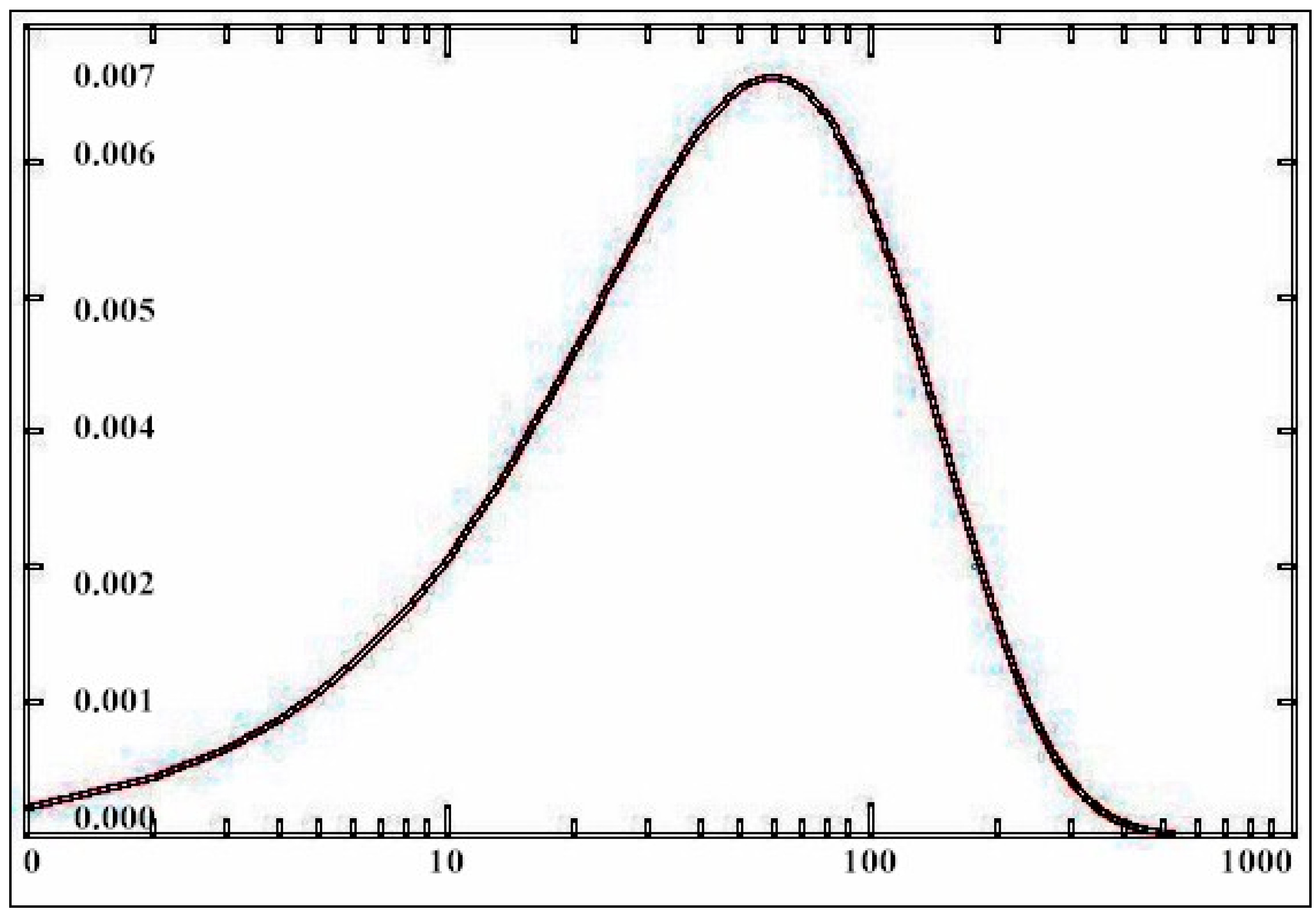
Figure 1.
At the sample
of the income density distribution,
solves the equation
for
;
.
Appendix A1 contains the analytical form for the sample expression in
Figure 1.
Figure 1.
At the sample
of the income density distribution,
solves the equation
for
;
.
Appendix A1 contains the analytical form for the sample expression in
Figure 1.
We thus present a theoretical model of visionary politicians, whereby we consider a masquerade of life or a scenario of realistic utopia. In this scenario, two actors/politicians, akin to two political coalitions, are playing a bargaining game, each attempting to implement his/her own wealth redistribution policy. Left-wing politicians tend to oppose the disproportion in private consumption, unjust wealth redistribution, profit motive, and private property as the main sources of socioeconomic evil. Right-wing politicians, owing to a different ideology, tend to focus on regulating business and financial risks, thus encouraging the government’s use of its powers in combating corruption, criminal violence and commercial fraud. While left-wing politicians prefer immediate and equitable sharing of the available stock of goods and services, both sides are aware of the citizens’ sacrifices—in terms of direct contribution of a part of their income to the funding of welfare benefits and public goods. We posit that applying the rules and norms of wealth redistribution pertaining to the reliance on the elevated relief would increase the quantity of the relief payments to be delivered. Consequently, citizens will have to meet a greater tax burden. This outcome is not ideal, given that lower tax burden and greater private consumption always lie at the heart of citizens’ economic and political aspirations. These private objectives prompt majority of voters, who hold power in electing political parties, to oppose increasing the tax burden. As a result, they are instrumental in the competition between the left- and right-wing politicians and their views on tax policies.
Political consensus is rarely possible in reality. Consequently, we aim to design an experiment capable of predicting an appropriate political division between interest groups for desirable implementation of the welfare policy. This approach does not require analysis of the voting system or a scheme by which voters-citizens express their arguments. In adopting this approach, we analyze political power indicators as replications
,
, in line with Kalai’s bargaining game [
8] in which the division of $1 is attempted. In this scenario, among other assumptions, it is posited that a power
is appropriate to adopt the ability to negotiate, or be in the position to request financial support to a greater extent than the opposite side. Similar interpretation of the players’ power dynamic may be found in the recent work of Mullat [
9]. In short, we adopted the view of Roberts, who noted in 1977 [
10] that “
The point is not whether choices in the public domain are made through a voting mechanism but whether choice procedures mirror some voting mechanism.”
These brief remarks should be sufficient to elucidate some goals of the state, allowing us to conclude that welfare policy in a representative democracy always faces ideological controversies of politicians and citizens. A further aim of this experiment is to shed light on how a political consensus is reached and whether it reflects a criterion of tax policy that results in the least burden to the citizens. To address this issue, as already stated, we focus our analysis on two visionary politicians. For the purpose of the experiment, we assume that these politicians are granted a political mandate to initiate proposals ensuring that the relief payments are allocated to citizens who are in need. We thus assume that, in balancing the books accounting for the finance of relief payments and for vital public goods and services, expenses are constrained. This premise ensures that the citizens control the negotiations, forcing the politicians to act within the imposed budget constraints in order to pledge safe funding for their proposals. While trying to reduce the after-tax income inequality, the politicians in their respective roles of left- and right-wing actors are committed to ensuring that the wealth is redistributed fairly.
At this point, it is essential to state the assumptions/limitations underpinning the analysis of a hypothetical behavior of those occupying three distinct roles in the negotiations—those of left- and right-wing politicians and voters-citizens. Throughout this work, we emphasize the incomparability between the aims of the left-wing politicians struggling to ensure adequate access to basic goods and the right-wing politicians advocating for availability of non-primary but vital goods and services. In the analysis, we implicitly assume that politicians do not have adequate knowledge of citizens’ needs in a more primitive environment. Hence, they can only work with the monetary payoff specification. Given this limitation, politicians are unaware that the provision of equivalently valued public services is not a perfect substitute. For example, we assume that politicians do not have any information on how household income is assembled and used to buy private health insurance or services of nursing housing, etc. Thus, we do not merit the debate on what is right or wrong in the economic or political environment involving left- and right-wing politicians and voters-citizens. In short, our work does not extend to the democratic context of voters’ prototypes/characteristics. While acknowledging the significance of prototypes, in this work, we view voters’ behavior as a binary process, allowing support for either left- or right-wing politicians. This, however, introduces a risk of premature political breakdown of negotiations. In addition, we refer to the tax revenue in accordance with voters’ preferences as the “wealth-pie” , which is divided into two parts , whereby denotes various social benefits or relief payments, and pertains to public goods, so that . We posit that any further enrichment of voters’ characteristics would disrupt the delicate balance between the motives of our experiment and the theoretical framework, which is already technically sophisticated.
Roadmap. Because of the narrative complexity, it is possible that the reader would find proceeding with the content of the paper in chronological order difficult. Thus, to mitigate this potential issue,
Section 3 presents the most relevant problems, in particular the pre-equity condition of political breakdown of the negotiations. In our view, it is prudent to master the material presented in
Section 3.1 before moving to
Section 4. Similarly,
Section 3.2 aims to assist with understanding of the content of
Section 5, while
Section 3.4 supports
Section 6. On the other hand, those not wishing to delve deeply into the technical aspects of this work could simply move onto
Section 7. Nonetheless,
Section 3.3 provides a scheme pertaining to the pre-equity of breakdown of the negotiations and, in our view, does not require further clarification.
2. Preliminaries
Before delving deeper into our work, we specify the category of the game payoffs functions
,
and taxes
required for the model validity. As noted above,
Section 3 provides background information that assists in understanding material given in
Section 4,
Section 5 and
Section 6. In
Section 4, we disclose fiscally safe welfare policy in amalgamation with imposed
budget constraints for financing relief payments. Referred to as volatility constraint, the amalgamation dynamically restricts the h-effect—an inverse working incentives phenomenon of low-income citizens. In
Section 5, citizens’ ambivalence and multifaceted welfare policy perceptions are discussed from the perspective of the alternating-offers game. The policy on poverty associates the left- and right-wing politicians with payoffs functions
and
. Under these conditions, it is possible to obtain an analytical solution to the game with incomes
density distribution
. Indeed, as will be shown, the calculus of indicators
complies with the political power design given in
Section 6. The results are discussed in
Section 7, followed by concluding remarks, presented in
Section 8.
In the current experiment, an income
equal to the poverty line
,
parameterizes all arguments and functions. In this vein, we adopt quantitative measurement, whereby we utilize a scale quantum as an average income with the income
density
distribution,
. The average establishes the ratio scale. Hence, we suggest that
(the after-tax residue of income
) signifies the first actor’s social position at the specified scale,
i.e., the left-wing political aims. We apply the residue formula based on Malcomson’s [
11] model, with a personal allowance parameter
,
, determined by the tax bracket
. The second actor’s aim—the right-wing political objective
—is ensuring a sufficient amount of the non-basic goods per capita. Here, we refer to the citizen
as
marginal citizen. While, for the minority of voters, the relief is more attractive than lower taxes, the third actor is the implicit partaker embodying the majority of voters whose preference is minimizing tax obligation
. This is a typical public finance dilemma of efficient division
of the tax revenue into shares
. In this work, the dilemma is represented by the alternating-offers bargaining game
with premature risk
,
, of political breakdown. When
, the solution converges into the Nash axiomatic approach [
12]. The relationship between the one that suggests the alternating-offers bargaining and axiomatic solution is well known from the work of Osborn and Rubinstein [
13]. As this game is thoroughly described by Osborn and Rubinstein, for brevity, no further elaboration is offered here.
When negotiating on finance issues, under the guise of a “
wealth-pie workshop”, politicians will allegedly try to divide the wealth-pie in a rational and efficient manner. As a result, the tax
will increase, as will the wealth-pie, when increasing the poverty line
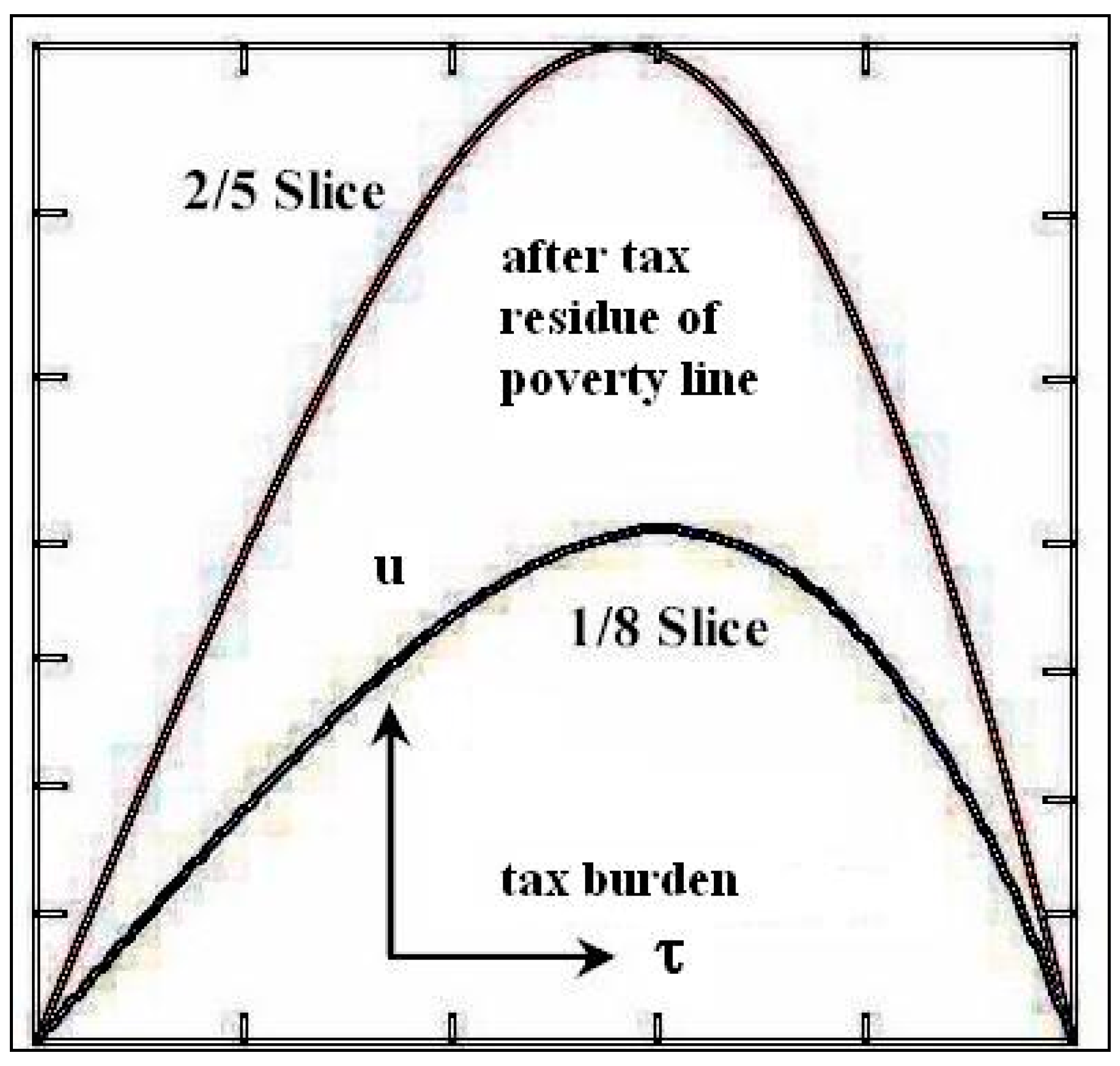
. Logically, a decrease in taxes would yield the reverse effect. While taxes vary, the division will depend upon the characteristics and expectations of the bargainers involved. Indeed, the left- and right-wing political aims
pertaining to basic goods, as well as the objective
related to the non-basic goods, are controversial. We illustrate this tax controversy by elevated single-peaked frontier of
, the
-share/slice in
Figure 2, which corresponds to the lower but progressively increasing concave frontier of
, the
-share/slice in
Figure 3, as well as for another division of the pie into shares/slices
. We believe, that, while
highlights the left-wing political aspirations, the share/slice
elucidates those of the right-wing political objective. This premise appears to be crucial for understanding our primary goal in resolving the welfare policy dilemma.
In support of the aforementioned assumption, the political payoffs in general, as shown in
Figure 2 and
Figure 3, emerge within a two-man economy endowed by citizens’ income abilities marginalized at the level of poverty line. According to Black [
14], single peakedness plays the key role in collective decision-making when the decision is reached by voting. The payoffs for the two actors, shaped in this way, are non-conforming,
i.e., incomparable, and are thus impossible to match through a monotone transformation, as established by Narens and Luce [
15]. The single peakedness is nonetheless in line with Malcomson’s tax residue
, when the terms of the contract commit the actors to shares
. This, however, requires that the expenses covered by flat taxes will balance the books while accounting for relief payments, as shown in
Figure 2. Clearly, increasing the poverty line requires an excessive increase in taxes, which in turn provides a greater amount of non-basic goods
, as shown in
Figure 3. An opposite scenario of increasing the available amount of non-basic goods
equally requires an excessive tax increase, which may lead to the possibility of an increasing poverty line.
Figure 2.
Left-wing politicians’ emphases.
Figure 2.
Left-wing politicians’ emphases.
Figure 3.
Right-wing politicians’ emphases.
Figure 3.
Right-wing politicians’ emphases.
Following the traditional procedure for the division of the wealth-pie in the alternating-offers game, when the pie is desirable at all the times, the politicians (bargainers)—changing roles—commit to shares
,
. According to the shares
, the valid rules and norms of wealth redistribution, which guarantee a desirable level of relief payments, require establishing a poverty line
parameter. However, an efficient division of the wealth-pie—as a result of single-peaked
-curves depicted in
Figure 2—no longer represents any traditional bargaining procedure. This is the case as, instead of division, the procedure can be resettled. Indeed, we can proceed at distinct levels of one parameter—within the poverty line interval
—reflecting the scope of negotiations. In fact, in 2007, Cardona and Ponsattí [
16] also noted that “
the bargaining problem is not radically different from negotiations to split a private surplus” when all the parties in the bargaining process have the same, conforming expectations. This argument applies even when the expectations of the first player are principally non-conforming,
i.e., single-peaked rather than concave. In our experiment, the scope of negotiations on the “contract curve” of non-conforming expectations allows for omitting the “Pareto efficiency” and replacing the axiom with a “well defined bargaining problem”, as posited by Roth [
17]. The well-defined problem
of the wealth-pie division can now be solved (resettled) inside the poverty line interval
.
Settings
In accordance with Friedman’s NIT system, in this work, we assume that, for the unfair subsistence of the less fortunate citizen
, the relief amount
,
, serves as a monetary compensation designated for purchasing an eligible "poverty basket" of food, clothing, shelter, fuel,
etc. According to Rawls [
5], “
primary goods are things which it is supposed a rational man wants whatever he wants.” In defining the parameter
in this manner, it becomes contingent on financing the relief. This can be achieved by assuming that elevating the poverty line
requires an increased marginal tax rate
. In increasing the wealth-pie through tax channels, we assume an acceleration
of the tax rate
;
inclusive all of those citizens who indicate the marginal income
denoted by
.
As noted previously, the marginal citizen must bear the cost of the left-wing political aims using tax residue , as well as the right-wing political objective , referred to as “public or non-basic goods”. With the proviso that politicians commit to the shares , we conclude that is a single -peaked curve, due to the tax rate increase upon . While objective of right-wing politicians decreases with an increase in , the reverse is true with elevating due to acceleration. Here, payoffs are considered analytic functions , . Given the interval , referred to as the scope of negotiations, reflects single -peakedness where upon increase, , . Following an increase in , the payoffs become convex, , , whereas an increase in would produce concave payoffs , with , . It can be shown that, with increasing , payoffs always decrease; in other words, in both circumstances, either is convex, or is concave.
3. Relevant Trends and Issues
In the extant literature [
18,
19,
20], the welfare, economic, and political issues are usually addressed in reference to specific questions. In our view, a much deeper analysis is achieved when addressing them more generally, adopting well-established knowledge discovery methodologies. In particular, our wealth-pie workshop concept, jointly adopting the four issues of (a) public finance; (b) alternating-offers game; (c) negotiations’ collapse analysis; and (d) political power design, leads to a more informative point of departure.
To explain the root cause of the results in order to bring the welfare, economic, and political content to the surface in a rigorous analytical form, and to find bilaterally acceptable solutions to the game, we will visit all of the classrooms in our workshop. Our goal is to lay the foundation for a more constructive welfare policy comprehending the meaning of the following four narratives:
Fiscal policy: During the delivery to its final destinations, provided that the books accounting for the relief payments finance have been balanced a priori, the wealth-pie must remain balanced throughout and in spite of volatility in the economy;
Negotiations: The left- and right-wing political bargaining on how to share the wealth-pie complies with the rules and norms of the alternating-offers bargaining game;
Pre-equity of breakdown: Political breakdown, or threat, directly affects the bargaining solution. Pre-equity guarantees equal conditions for players before the bargaining game commences;
Political power design: Bringing a motion to a vote is necessary to address the majority opposition to high taxes and excessive public spending. Whether it is viewed as positive or negative, or whether it ought to be acknowledged or not, rejected or accepted, this motion must be politically designed in advance.
In our wealth-pie workshop, these four narratives can be understood as obligations/constraints to be met by welfare policy rules and norms, akin to the “Rational man” deliberation of Rubinstein [
21]. This interpretation allows us to provide a scenario under which the narratives are embedded into the welfare policy of the state. In addition, evaluating the welfare policy from this perspective reveals that the analysis can be subject to and performed by computer simulations, as shown in
Appendix A2. Our initiative could also serve to unify the theoretical structure of the economic analysis of public spending. Moreover, it can be used to evaluate the political power design of left- and right-wing politicians, or to conduct systematic inquiry into impacts of governmental decisions and actions on wealth redistribution.
As the state has the duty to help the less fortunate, our experiment approaches wealth redistribution in a two-fold manner. First, it addresses the provision of basic necessities or goods, such as shelter and heating, clean and fresh water, nutrition,
etc., before focusing on non-basic goods, including national defense, public safety and order, roads and highway systems, and so on. In regard to welfare policy issues, according to Boix [
22], “
…There is wide agreement in the literature that governments controlled by conservative or social democratic parties have distinct partisan economic objectives that they would prefer to pursue in the absence of any external constrains.” Meeting this challenge, based on income
density distribution
, we identify an effective approach to the division of
into shares
pertaining to basic goods
and non-basic goods
. Fundamentally, the efficient division
of the wealth-pie aims at just and fair delivery of all aforementioned goods, traditionally perceived as public goods. In our experiment, we refer to public goods as non-basic but vital goods, whereas basic goods are deemed fundamental. Incidentally, during the delivery of basic and non-basic goods to their end destinations, we treat both as public goods.
We assume that the left-wing politicians have the necessary political power—when an offer is made, irrespective of its legitimacy—to control the redistribution of basic goods independently. Given the single-peaked aspirations of the left-wing, in contrast to the objective of their right-wing counterparts, the power the left-wing politician enjoys is supposed to be adequate enough to reach the peak of these expectations. In particular, we believe that, beyond some peak position, inefficient usage of basic goods would lead to an excessive decline in the quality of welfare services, as well as cause deterioration in access to public goods for all citizens. In making these suppositions, we agree with Rawls’s [
5] statement about the precepts of perfect justice: “
The sum of transfers and benefits […] from essential public goods should be arranged so as to enhance the emphases of the least favored consistent with the required saving and the maintenance of equal liberties”.
An efficient usage of public resources implies that a consensus between left- and right-wing politicians might be reached. Despite some views to the contrary [
23], we posit that the bargaining aimed at finding a just and fair division of basic
vs. non-basic goods is an acceptable path to the bargaining dynamics. Based on this premise, we can identify relevant connections in extant works on economic and political behavior that analyze the sociological and political aims of ensuring adequate welfare by using public finance. This is likely be the best starting point for visiting our wealth-pie workshop.
3.1. Fiscally Safe Welfare Policies, to Be Continued in Section 4
Public finance focuses on the revenue side of tax policy. In particular, it pertains to the budget formation, as noted by Formby and Medema [
24], aiming to provide a guaranteed level of welfare to citizens endowed by poor productivity. While the welfare policy is a separate issue, it should be considered on the grounds of legal and moral rights of citizens. Empirical evidence confirming that such policy is government’s legal obligation can be found in pertinent literature. For example, as noted by Saunders [
25]: “
…poverty line. The line was initially set (in 1966) equal to the level of the minimum wage plus family benefits for one-earner couples with two children.” Similarly, a hypothesis consistent with moral obligations can be found in the literature of economic politics [
26,
27].
In 1959, Musgrave [
28] examined two basic approaches to taxation: the “
benefit approach” and “
ability-to-pay”, which put taxation into efficiency and equity contexts, respectively. In this work, we utilized the benefit approach in order to augment the existing standard of welfare policy, whereby we allocate a guaranteed amount of income for minimum taxes. We posit that a flat tax system—based on injecting optimal equity according to the ability-to-pay principle of “proportional sacrifice”—ensures that taxes remain
fairly levied.
Taxation is a principal funding source of social costs and benefits. Thus, the first postulate in our welfare policy workshop (see above) discloses an obvious paradigm in social policy. According to the ability-to-pay principle commonly adopted in public finance, in order to stabilize the distortion of tax policies, the known terms of warranty must rely on exogenous taxes enforced on the productivity of citizens. The concept, proposed in 1996 by Berliant and Page Jr. [
29], is a variant of the classic public finance and similar approaches, applicable when an agent characterized by a specific level of productivity does not shift his/her labor supply after all adjustments to the tax formula have been implemented. In other words, under this paradigm, optimal taxation enforces optimal labor supply.
Yet another “treatment of policies”, closely related to societal instability, entails equity of pre- and post-tax positions of citizens. Such a view demarcates between citizens and has attracted the attention of economists and tax policy-makers. In the view of Kesselman and Garfinkel [
30], credit tax-scheme analysis opposes the income-tested program in the rich and the poor, also known as two-man economy. Poverty measurements have also been addressed in the works of Sen [
31], Atkinson, [
32], Ebert [
33], and Hunter
et al. [
34]. According to Tarp
et al. [
35], “
The poverty line acts as a threshold with households falling below the poverty line considered poor and those above poverty line considered nonpoor.” In 2008, Peñalosa [
36] investigated wealth redistribution as a form of social insurance in relation to economic growth. On the other hand, Stewart
et al. [
37] attempted to reduce horizontal inequalities, proposing “
a reallocation in the production, operation and consumption of publicly funded services”.
In the attempt to assess and control the circulation of wealth through tax channels, we argue that, unless fiscal stabilization is not a required condition when justifying public spending, it will be difficult to explain how the citizens eligible for relief gain access to the benefits and relief payments. Thus, while we continue to rely on fiscal stabilization, in order to highlight a particular type of the dynamics stability, we refer to welfare policy as idempotent. For clarity, a choice operation (or decision) applied multiple times is deemed idempotent if, beyond the initial application, it yields the same result [
38]. Thus, based on this dynamic definition, the idempotent scheme allows the politicians to honor the pledges made during the election campaign as, once the political decision is taken, it eliminates the need for further stabilization. While visiting the workshop, the circulation of wealth is supposed to be dynamically stable,
i.e., it is idempotent.
3.2. Bargaining the Welfare State Rules and Norms, to be Continued in Section 5
Bargaining is the key element of economics and is at the core of politics. On the other hand, as pointed out by North [
39], “
The interface between economics and politics is still in a primitive state in our theories but its development is essential if we are to implement policies consistent with intentions.” More recently, Feldstein [
40] noted, “
Unfortunately, there is no reason to be pleased about the analysis in policy discussions of the efficiency effects…of the welfare consequences of proposed tax changes.” Similarly, in a review on “Handbook of New Institutional Economics”, Richter [
41] stressed,
“…that the sociological analysis…and large institutional structures in economic life is still at an early stage…game theory, and computer simulation could help to further develop the new institutional approach…game theory might be a defendable heuristic device of NIE.” Indeed, the left- and right-wing politicians, like actors in the game, strive to implement their vision of the state welfare institutions. This is succinctly explained by Ostrom [
42], who noted, “
These flimsy structures, however, are used by individuals to allocate resource flows to participants according to rules that have been devised in tough constitutional and collective-choice bargaining situations over time.”
In order to achieve the aforementioned vision of collective choice, it is appropriate to consider a scenario in which the actors/voters play the “bargaining drama” of economic and political issues. Bargaining has been a theme of a wide range of publications, including the work of Alvin E. Roth [
43]. Despite the simplification, the binary behavior of voters remains at the root of the democratic transformation of public institutions. In this regard, binary position fits particularly well into the bargaining game with exogenous risk
,
, of breakdown [
13]. Actually, bargaining can be risky for all interested actors because they may lose voters to the competition if their terms are not met. Thus, it is essential to first clarify the political power dynamics of both the left-wing and the right-wing politicians. Henceforth, they are respectively referred to as LWP, the first actor, benefiting from a power
,
, and RWP, the second actor, benefiting from a power
.
Numerous factors—such as economic growth, decline or stagnation, demographic shift or pit, political change or change in scarcity of resources, skills and education of the labor force,
etc.—might create fiscal imbalance in a desirable welfare policy due to the transfers of benefits and relief payments. As a result, the size of the wealth-pie might be too small (
i.e., not worth the effort required for its redistribution) or too large (introducing mutual traps) to achieve a stabilized public spending mechanism. In either case, the actors may decide not to share the pie at all. To address this controversy, as previously underlined, we assume that politicians participate in relevant public institutions. If the institutions cannot or do not want to follow RWP’s policy of wealth redistribution, RWP—in order to promote their own understanding—can be sufficiently legitimate to deliver the wealth “properly”. In doing so, RWP can enforce vital decisions by several means, including resource mobilization, retaliation for breaches and criminal fraud, recruiting political volunteers and managing public service commissions, soliciting private contributions,
etc. In other words, as Kalai [
8] pointed out, RWP would rely on an “
enthusiastic supporter”. On the other hand, as LWP face a decay in political legitimacy for perfect justice, they cannot fully control RWP’s actions and intentions when their political interests in the final agreement are incomparable. In these circumstances, RWP are aware that their abilities and access to information might necessitate agreeing with, or at least not resisting, LWP’s privileges to make arrangements upon the size of the pie. Hence, from the RWP’s critical point of view, whether acting politically in common interest or not, it might be prudent to acknowledge LWP’s welfare activities. This elucidates the asymmetric dynamics of the political power division between the LWP and RWP.
Returning to the main points of asymmetric bargaining, we will illustrate an efficient solution
by the division of $1 aimed at maximizing the product of actors’ payoffs above the disagreement point
:
Although game theory purists might find the solution clear, the questions asked by many often include: What are
,
,
,
, and
? What does the point
mean, and how is the
formula used? The simple answer, as initially provided by Kalai [
8] as an asymmetric variant of the Nash [
12] problem, is as follows:
- • X
is the first actor’s share of $1, with as the first actor’s asymmetric power indicator, , ;
- • u(x)
denotes the first actor’s payoffs of the first actor’s $1 share ;
- • y
is the second actor’s share of $1, where is the second actor’s asymmetric power indicator, ;
- • g(y)
denotes the second actor’s payoffs of the second actor’s $1 share .
Based on the widely accepted nomenclature, we refer to as the utility or payoffs pair. Thus, the disagreement/threat point represents the payoffs the two actors obtain if they cannot agree on how to share the wealth-pie. In the same vein, represents the disagreement or breakdown point, whereby the players collect nothing.
In the subsequent sections, we will provide an analytical solution exploiting payoffs in the form
and taxes in the form
within the scope of negotiations
comprising the endpoints of the interval
. According to the analytical solution, implicitly hiding the variables
, it follows that any negotiation of shares
can be perceived as two sides of the same bargain’s portfolio, as the shares
are accompanied by poverty lines
. While hiding the variables
,
, we may respond to the question of whether solution
is efficient in a traditional sense. Indeed, akin to the above, political bargaining can now be expressed by poverty line
maximizing the product of political payoffs above the threat point
:
On the other hand, unlike the traditional threat point , the public/vital goods amount in the game—the component of the point —might be negative. This will apply in our experiment of a breakdown of negotiations, whereby funds need to be borrowed or acquired through other means in order to balance the books and account for the welfare expenses—a situation of “genuine negative taxes”. It is important to note that, while this may seem counterintuitive to some readers, in the theory of public finance, the use of genuine negative taxes is not prohibited.
Finally, we conclude that, all these remarks notwithstanding, it is irrelevant whether the players are bargaining on shares
or trying to agree on the poverty line level. This assertion highlights the main advantage of hiding the variables
. In particular, it brings about a number of different patterns of outcome interpretations in the game, such as linking an outcome to the lowest tax rate, which is the most desirable sacrifice of voters’ majority. In consideration of alternative approaches—which describe outcomes of collective bargaining in the form of voting, or partaking in any voting scheme in the form of bargaining—the scope of negotiations
brings the voting and bargaining schemes into the same context, as both can be enriched by adopting this approach. Our insight is forward-looking in the sense that it aims to identify an alternative-offers game solution, whereby both actors accept at once the proposals (moves) made by the other side. Our initiative approach could also serve to unify the theoretical structure of economic analysis of the productivity problem. Indeed, when referring to Leibenstein’s work [
44], Altman in [
45] noticed:
Leibenstein argued that there are two components to the productivity problem: one relates to the determination of the size of the pie, while the second relates to the division of the pie. Looked upon independently, all agents can jointly gain by increasing the pie size…the situation need not be a zero-sum game. Tactics that determine pie division can affect the size of the pie. It is this latter possibility that is especially significant.
3.3. Pre-Equity of Political Breakdown
Beyond the asymmetric dynamics, the game inherits a
premature disagreement or breakdown point, similar to that discussed by Osborn and Rubinstein [
13]:
We can interpret a breakdown as the result of the intervention of a third party, who exploits the mutual gains. A breakdown can be interpreted also as the event that a threat made by one of the parties to halt the negotiations is actually realized. This possibility is especially relevant when a bargainer is a team (e.g., government), the leaders of which may find themselves unavoidably trapped by their own threats.
In our game, the asymmetric solution incorporates the left- and right-wing political power indicators into a breakdown policy. In order to be addressed properly, the indicators cannot be given exogenously. To overcome this obstacle, we introduce a policy of endogenously extracted breakdown into the game, based on a condition referred to as the pre-equity of political breakdown.
Traditionally, in the alternating-offers game, the breakdown corresponds to two standard pairs of payoffs
, or in the words of Osborn and Rubinstein [
13], “
to the worst outcome.” In the left- and right-political bargaining, due to the implicit pressure from the voters, as both politicians aim to find—at least from their perspective—a just and fair solution, there will always be a temptation for binary voters to defect to the other side. This puts the negotiations at risk
of a premature collapse. Even under the worst circumstances, in the event of collapse, the quality and the size of the wealth-pie should be equal for both politicians. This premise holds in these unfavorable circumstances as the entire pie will be decided upon by one of the politicians. Thus, when the premature collapse occurs, it is important to arrange the terms of contract in such a way that neither politician can exploit or misuse these adverse circumstances to his/her own advantage. To meet this condition, when normalizing the standard breakdown under the description valid for the alternating-offers game
, we are working toward an endogenous form for equity in accordance with political non-conforming expectations.
As stated, the standard case of breakdown in the alternating-offers game corresponds to two pairs of payoffs. In this form, the breakdown is generally found using ex-ante linear transformation, namely the exogenous normalization of utilities. When the collapse is imminent, the political breakdown exposes the equity condition pertaining to the actual event of breakdown. Unlike the standard case, once the most unfavorable result occurs, the resulting collapse must include additional parameters—the tax and the wealth . In order to equalize—or endogenously normalize—the breakdown, the politicians involved in negotiations can make a priori arrangements, or sign binding agreements upon these two parameters, i.e., and . Without availability or warranty of such a pre-equity, an endogenous normalization is unrealistic. In the view of the voters’ electoral maneuvering (discussed in the next subsection), even if the pre-equity normalization is not always achievable, it is more constructive to determine the breakdown according to some rational context.
Before proceeding further with a detailed assessment of the aforementioned definition, we recall the concept of wealth amount , redistributed by the state as the average taxable income per capita, scholarly defined as “prosperity or a commodity”. Next, according to the conditions characterizing the collapsed environment, at the start of the negotiations, the draft of a contract includes both taxes and—in line with our nomenclature—the wealth amount . The product identifies the size of the wealth-pie within an interval within the scope of negotiations, thus establishing the boundary for the two politicians. The lower limit denotes the initial proposal, which is the most attractive for RWP, while being the most unattractive for LWP. In the same but inverse order can be paired with . Having set these limits, we can proceed with examining how the breakdown might be conditionally, albeit endogenously, encoded into the game.
Indeed, we now contribute to implementing our wealth definition of how the breakdown can be established endogenously. To do so, we consider a situation driving the welfare policy in the context of cost-benefit equity. When the collapse of negotiations is imminent, the differences in the amounts of wealth and taxes for funding low-cost welfare policy
against an expensive policy
,
—
i.e., funding payoffs
for
against
for
,
,
—can amplify misunderstandings and contribute to traps. At the endpoints of the scope
, the wealth-pie sizes
and
at poverty lines
and
can require the delivery of wealth amounts
and
, albeit at different prices, represented as taxes
and
, according to Buchanan [
46]. Hence, prior to the start of the game, and in line with the cost-benefit equity, in the most adverse circumstances, the payoffs
and
should preserve equal prices
for the delivery of equal amounts
of wealth. Such a market-driven interpretation of
commodities delivery to the end destinations relies heavily on the size of the wealth-pie, which is equal to
. It should be noted that this interpretation is only relevant to the case of flat (proportional) taxes.
To explicate the interpretation of reasoning in the previous lines, it is worth examining the “well defined bargaining problem”, depicted as the contract curve in
Figure 4. Based on the discussion presented thus far, our goal is to set an interval
solving two non-linear equations,
and
, by attempting to find a cross-point
where the curve crosses its own contour, as
YX-axis coordinates, on the plane with
, which is equivalent to the roots
and
. Although the calculus of the point
does not extend beyond high school mathematics, it does not confirm the possibility of normalization in general. This, however, does not invalidate our discussion, as we do not claim that the equity condition can be achieved in all circumstances. It should still be pointed out that, in a number of examples where the validity of the condition was detected, we found a breakdown endogenously encoded into the game, indicating normalization in the form of
.
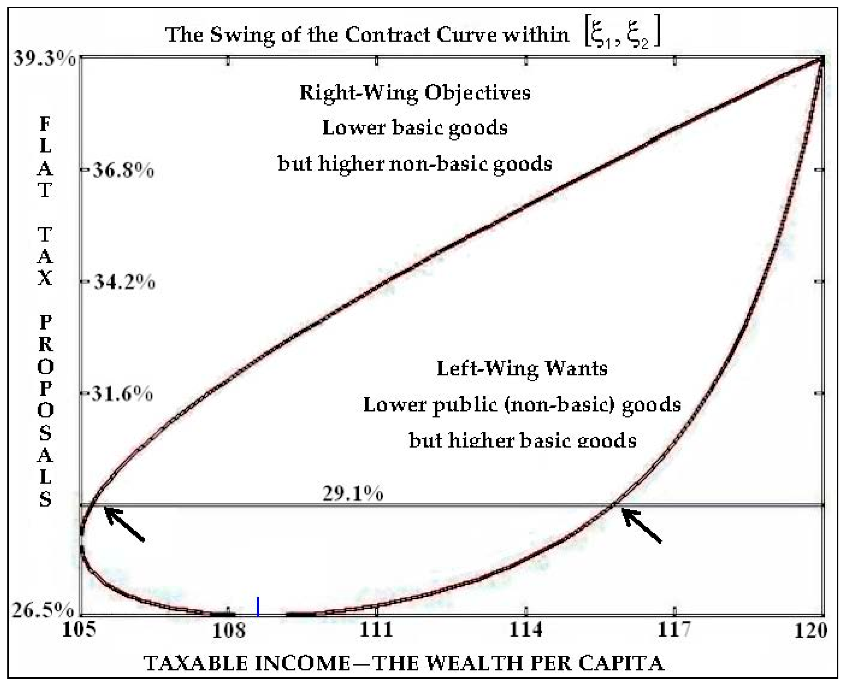
Figure 4.
The graph depicts two different motions for a vote. For the higher tax τ = 29.01%, marked by the horizontal line, and the lowest tax τ = 26.52%, marked by the vertical dash. Indicated by , at cross-points of the contract curve with the horizontal line, we observe controversial expectations of voters. The shares of lower basic but higher public goods are shown on the left, while this payoff reverses towards the right side of the graph, as the shares of basic goods increase while those of public goods decrease. Thus, the higher tax τ = 29.01% cannot lead to a political consent, in line with Observation 5.
In line with the above, as the aim is to bring the politicians, if possible, into just and equal positions prior to negotiations, and equalizing taxes and wealth amounts in the collapsed environments and might be a rational starting point. Under this premise, endogenously encoded into the game, we label the equity condition, as a pre-equity of political breakdown. If valid, this condition equalizes fiscally realistic and just demands for public spending prior to negotiations, in particular the size of the wealth-pie .
3.4. Voting and Political Power Design, to Be Continued in Section 6
Only the voting results can reveal the true incentives of people that will give the democracy its final judgment. The voting process is the only avenue for the voters to assume the roles of current or upcoming politicians to whom the opportunity will be granted in line with the population’s aspirations to redesign the rules and norms of wealth redistribution. Voters’ inequalities, life plans, background, social class and experience, native endowments, political capital, etc., determine the bulletin collected at the voting table. Consequently, incongruence in voters’ views or interpretations of reality affects the individual choices and thus the voting results, thereby influencing political pre-election campaign. Voting results are not fully predictable due to the deviations in voters’ views and opinions on how the wealth redistribution ought to be achieved. The problem stems from the fact that welfare policy proposals that benefit the minority of citizens sometimes require higher taxes. On the other hand, the majority of voters would be primarily guided by selfish attitudes toward lower taxes, which would implicitly affect the political bargaining positions. Such an attitude likely deserves a critical examination. Given these arguments, our question is: Why should the left- and right-wing politicians care about lower taxes?
It is timely to recall political outmaneuvering with an implicit risk
,
, upon negotiations suffering a premature collapse. Indeed,
Figure 4 depicts the contract curve of efficient public policies/proposals
upon poverty lines in the bargaining game
. Politically rational and economically effective proposals
, forming the curve, have been projected onto the two-dimensional space of the tax rate
and taxable income—the wealth amount
. Although the payoffs
are embedded in each point, they are not visible on the graph. These invisible/hidden payoffs in the upper part of the graph symbolize the wealth-pie division
into lower basic
yet higher of public goods shares
, as left-wing politicians aim for
, whereas those in the right-wing political party aspire towards
accordingly. Similarly, the payoffs in the lower part symbolize a reverse situation—the higher basic
vs. lower public goods, as shown in
Figure 2 and
Figure 3. Thus, once all views are represented, the political payoffs
for pledged tax hikes
are more favorable for some coalitions of voters compared to others. As voters’ preferences for the balance between basic and public goods vary, the approach to determining the efficient poverty line resulting from eventual agreement between politicians is two-fold. Indeed, unless the tax hikes are excessively high, the
upper coalitions’ representatives will always try to outmaneuver the
lower coalitions’ representatives. The politicians are aware of this dynamic when taxes are high. As they feel trapped in negotiations, binary voters become more likely to defect to the other side, putting the negotiations at risk
of a premature collapse. In contrast, when taxes are sufficiently low, the range of eventual voters’ electoral maneuvering will substantially reduce or even vanish. The lowest tax is likely the one that yields desirable outcomes for the majority of citizens.
In the line of reasoning that concerns the majority of citizens, it is appropriate to address the design of the political power indicators . Considering the bargaining outmaneuvering of left- and right-wing politicians according to the alternate-offers game , we state that the politicians on the opposite sides of the bargaining table might disagree with respect to the terms of the outcomes. Consequently, they would delay the decision while consolidating a draft of a consensus document. This document might not necessarily yield the best outcome for the citizens, who represent the majority and are of view that the policy that minimizes taxes is always the most desirable choice. Despite knowing that the majority will never endorse higher taxes, the minimum tax rate might not necessarily be a desirable outcome from the political perspective. Thus, politicians may choose to disregard the majority interests because the political power of LWP or RWP, as rational actors/politicians, might be strong enough to negotiate selfish decisions that are beneficial only for them. In order to entice politicians not to act selfishly, as this would likely result in the ultimate collapse in the negotiation process, their political power indicators ought to represent a natural power consensus motivating them to choose a desirable outcome for themselves and for the majority of citizens—a platform that should ideally be designed in advance. This completed our preliminary investigation of the problem.
4. Analysis of Fiscally Safe Welfare Policies, Continued from Section 3.1
Delivery of basic goods, which counteracts negative contingency, if it occurs, is the main political responsibility of the left-wing actors. Herewith, the left-wing political intervention is of the greatest political importance. It is universal in the sense that it pertains to all citizens, irrespective of individual situation before or after the contingency. Under this premise, basic goods that are available to citizens are of sufficiently high quality and poverty is not allowed, as stressed by Greve [
47]. This course provides a relatively high level of welfare spending and taxes, creating misbalance in the books accounting for public finances, thereby introducing volatility conditions into the wealth-pie delivery. Hence, secured largely independently of market forces, the high level of basic goods might have a conflict-driven effect on the welfare policy, which should not be borne solely by citizens as, as already noted, the state has a duty to help the disadvantaged.
Assuming that the conflict-driven welfare policy guides our political actors in trying to reach an agreement, the left-wing politicians should aim to secure an efficient size of the wealth-pie. Thus, LWP prescribe the size of the pie and propose the division method which the right-wing politicians accept or reject. If rejected, the RWP would suggest their preferred division, while only having the authority to recommend a size that the LWP might not be obligated to accept. We also assumed that, upon delivery to its end destinations, the wealth-pie remains fiscally safe, i.e., it does not change its size. Under the rules of the alternating-offers procedure (see later), the game will continue until a consensus is reached. This process presupposes that left-wing politicians are committed to the share of the pie, while not being committed to the size.
Let us now envisage a contrasting scenario whereby the public spending increases. Hence, both actors know that, upon delivery, the size of the wealth-pie might change. This, in turn, leads to a misbalance between the relief payments, which can put the pie size in doubt or make it even more difficult to ascertain. As a result, the difficulty related to political pledges might force both sides to retreat. In such volatile conditions, the wealth-pie is no longer fiscally safe and might affect the expectations of both politicians. Consequently, a fiscally safe plan in spite of volatile conditions for the delivery and division of the wealth-pie is needed. Otherwise, unless welfare policy fails to enforce fiscal safety, the rules and norms of the relief payments are not living up to their claims. In other words, having a criterion for determining whether a welfare policy is fiscally safe is necessary.
It is helpful to focus first on welfare policy without any warranty of fiscal safety. It could, for example, be determined by the poverty line , identifying the recipients of wealth redistribution. When is low, the variable , , allocates the income of the needy or the benefit claimants. In this scenario, the benefit claimant claims and receives a relief payment proportional to , i.e., , as previously discussed. In this scenario, all other citizens—both the wealthy and those with marginal income, denoted as and , respectively—receive no relief payment.
Next, we study a specific scheme highlighting the readiness of the society to fund welfare and public spending. For this analysis, we assume that the average cost
of the relief payments and the average taxable income
both depend on the poverty line parameter
,
,
—this is realistic, as shown in
Appendix A1. As previously scholarly defined,
can refer to the wealth amount. Based on our perception of income
density
distribution samples, the product
estimates the average tax revenue. Let the average cost of public goods be
, whereas the size
of the wealth-pie equals
,
. We assume that welfare and public spending reached the intended recipients, whereby the total spending equals
. This suggests that the basic and non-basic goods have been delivered to their final destinations. In other words, the wealth collected through tax channels is spent.
Now, let us assume that politicians in the game preferred to commit to the shares fixing , and might agree to hold the balance of the books accounting for financing the relief payments . That is, the left-wing politicians must be ready to finance the relief, i.e., to deliver by dividing the wealth-pie . In this scenario, the politicians pledge to retain the balance of the relief payments between credits and debts as a portion of the wealth-pie . The balance also specifies the welfare policy —an implementation of the poverty line , welfare reform, pact, program, etc. While the aforementioned balance is initially valid, it might not be in the future, putting the adjustment in on the agenda either once or repeatedly. Thus, the policy might represent a problem of fiscal imbalance. Almost all citizens, even if for different reasons, will prefer the opposite in the long run—a fiscally safe policy . For this reason, we now shift the focus on examining a constraint that corresponds to the fiscal safety of welfare policy , identifying—what we called above as idempotent—the safe delivery of the wealth-pie to its end destinations.
Idempotent Rules and Norms of Wealth Redistribution
The delivery of basic and public (non-basic) goods does not necessarily safeguard the funding of the expenses. As the expenses neither match nor prevent taxation hikes, the size of the wealth-pie could vary too rapidly. This leads, as previously discussed, to numerous adjustments of welfare policy rules and norms. To mitigate this issue, we have to examine the sequence
of multiple adjustments of the poverty line
. This highlights the fact that, on delivery, no adjustments of the wealth-pie are desirable. Consequently, it is better to keep the size of the pie unchanged,
i.e., fiscally safe. In other words, when replacing the old policy
with
, the two must coincide. Similar schemes, known as
idempotent, stem from bounded rationality mechanisms [
21,
38]. This premise suggests that, even if welfare policy rules and norms are subject to multiple adjustments, these adjustments should not change the
machinery of relief payments. In particular, when implemented twice, the rules must produce the same outcome. To guarantee the fiscal safety of the poverty line, such an understanding requires that the poverty lines must coincide amid a sequence of pairs
at some matching policy
.
The need to balance the books accounting for the delivery of relief payments , in spite of the wealth-pie volatility, can also be seen as immunity for financing the welfare policy. In particular, the immunity restricts, or at least realistically limits, the h-effect of wealth redistribution. Given the immune, i.e., fiscally idempotent, composition , the idempotent scheme is equivalent to implementing the policy only once. For this reason, we assume that the rules and norms of the relief payments have been socially planned and redesigned accordingly.
In this idempotent mode that outlines the fiscal safety of public spending, the rules and norms must reflect idempotent policy which brings the spending policy into focus. We conclude that the expenses designated for welfare spending must be in balance not only for funding relief payments , when the particular policy takes effect, but the policy must also enforce the fiscal safety in the full spectrum of current and future events.
Clearly, the balance is a static relationship leading to functional dependency that links the arguments and . Hereby, the tax rate becomes a function of and , expressed as . According to rules and norms in force of relief payments, the post-tax residue of the marginal citizens’ comprises fiscal limitations of wealth redistribution, while determines the personal allowance parameter, as shown above. The dependency transforms into a fiscally realistic social position . Irrespective of the current expenditure on basic goods, the real cost of living does not necessarily match . Hence, ensuring realistic and fiscally idempotent rules and norms, and/or, in particular, attempting to avoid the h-effect of this mismatch or adopt rules to keep the effect tolerable at least, an equation for a fiscally idempotent policy should be solved.
Observation 1. Constraint on left-wing political aims is necessary for upholding idempotent fiscal rules and norms of the imposed budget constraint .
According to this observation, whatever tax increase is implemented, the poverty line residue of the marginal citizens’ is unfeasibly high and cannot be attained when the condition has been violated.
Corollary. When
solves for
, the subsequent adjustments
are unnecessary. An option to change their welfare positions is irrational for citizens with incomes
or
; thus, the root
restricts (realistically limits) the h-effect. All pertinent proofs are given in
Appendix A3.
The fiscally idempotent policies
induce the basis for solutions in our game as fiscally idempotent compositions
. A reasonable question thus emerges:
Which taxable income characterizes fiscally idempotent welfare policies for the delivery of relief payments ? The answer is provided in the form of the following three constraints
1:
Taking the expression
out of constraint (2) and replacing
into
, the constraint given in (3) can be resolved with a fiscally idempotent policy for
, thus yielding:
Referred to as the volatility constraint, constraint (4) determines the fiscal safety module. It holds down the h-effect, amalgamating constraints (2) and (3) by balancing the books accounting for relief payments.
Summary. The outcome
constitutes the citizens’ bargaining shield for wealth redistribution which relates to a bundle of arguments or constants:
are controls, and
are status variables,
2 while
are the competing political proposals:
- ϕ
the personal allowance establishing the tax bracket ; it is an ex-ante control (tuning) variable, ;
- ξ
the income frame, the poverty line; a policy determining who is living in poverty, as well as the choice or the control parameter;
- z
the size of the wealth-pie; the amount of the wealth-pie that is equal to public spending per capita when taxes are proportional;
- X
the share of the wealth-pie of size z; a portion of z to be deposited in favor of the left-wing politicians for funding the relief payments, ;
- α
the political power of the left-wing politicians, ;
- τ
the marginal tax rate, the rate of the wealth amount determined by (1);
- u
the after-tax residue of the income frame equal to the poverty line , the wants function of the left-wing politicians, as determined by (2) and (3);
- g
the objective function of the right-wing politicians, determined by (1) and (2); the account for the refund of public goods expenses per capita.
The share and the marginal tax rate , due to the constraints 1 through 3, become functions of arguments : and . This form of dependence appears next in the module of the alternating-offers bargaining game.
5. Analysis of the Welfare State Bargaining and Rules and Norms, Continued from Section 3.2
Suppose that politicians, in pursuit of their commitments to a fair division of the wealth-pie, agreed to play the alternating-offers bargaining game
[
13]. In doing so, rational politicians are motivated to align the procedure to participate in any eventual agreement. The risk
of a premature collapse during negotiations, especially early in the game, might be the driving force behind their commitment to reach a consensus. Once a consensus on division is reached, they must agree on who will determine the size of the pie. Politicians negotiate on such matters when there are equal and symmetric preconditions in place that guarantee their equal rights. Thus, both will play an equal role in the decision regarding the pie size. Considering the right-wing vital political objective of wealth redistribution, it will be realistic to reduce the scope of RWP’s duties concerning welfare matters, while allowing them to retain their advisory rights. Our subsequent discussions are based on this premise.
5.1. Left- and Right-Wing Politicians’ Bargaining Procedure
Previously, we emphasized that, in a representative democracy, the division of the wealth-pie will always be subject to controversy. Recall that we consider two politicians: one acting in the role of LWP, who is aiming to provide basic goods to all citizens, and the other, representing RWP, advocating for the availability of non-basic goods. A precondition for the bilateral agreement is that the expectations of these two politicians depend solely on efficient policies of the LWP within the framework aimed at setting the poverty line
. However, politicians are more concerned with shares
than they are with the size of the wealth-pie. As a consequence of this independence, the efficient poverty line
provides shares related to efficient divisions
. Accepting this precondition, the RWP will only propose an efficient line
, as failure to do so would result in all other shares being rejected with certainty by LWP. Nonetheless, it is realistic that the RWP would—by negligence, mistake or some other reason—recommend an inefficient poverty line
, which the LWP would mistakenly accept. It is also possible that, in a reverse scenario, the LWP would choose to disregard an efficient recommendation
. This would be an irrational choice as, in any agreement, regardless of the underlying motives, both politicians are committed by proposals to shares
. Indeed, within the scope of negotiations
, the recommendation
concurs with RWP’s efficient share proposal
. Consequently, accepting
, while shifting LWP’s
mistakenly to
, at which both politicians must be committed to
, the shift
becomes inefficient and thus superfluous. Hence, making a proposal, the RWP’s recommendation on poverty lines makes a rational argument that the LWP must accept or reject in a standard way. Such an account, in our view, explains that the outcome of the bargaining game might be a desirable poverty line
. Hereby, the interval is referred to as the scope
of negotiations or bid proposals that are now, by default, linking the efficient lines
with shares
. The bargaining occurs exclusively in the interval
as a scope for efficient lines
of most trusted policy platforms for negotiations, where both players would either accept or reject the proposals. Political competition, depending on
, arranges a contract curve
(shown in
Figure 4 and
Figure 5) as a way to assemble the bargain portfolio. Given that the portfolio “has changed its color from shares to lines”, the politicians can now conceive themselves as making poverty line proposals. If a proposal is rejected, the roles of politicians change and a new proposal is submitted. The game continues in the traditional way by alternating offers.
Figure 5.
The aspirations of left-wing politicians expressed when opposing the right-wing political objectives are depicted on the vertical and horizontal axes, respectively. The graph shows the contract curve sloping from toward , projected on the surface of basic goods vs. vital goods—the projection of efficient poverty lines resolving the contract constraint (5).
5.2. Alternating-Offers Bargaining Game Analysis
We now proceed to a more accurate analysis of the game rules. Although the rules can be perceived as fiscally idempotent, the game itself contains a new challenge. The elevated poverty line
does not necessarily increase the marginal citizens’
after-tax residue
. The low-income citizens—the benefit recipients—can claim relief payments, whereby an increased number of claims might have a reverse effect on
, which would consequently decline. Indeed, in contrast to the increasing poverty line
and despite the required unavoidable increase in taxes—as the hazard (h-effect) is still present—in this scenario, the residue
will decrease. With the proviso that the left-wing politicians commit to the share
, the right-wing politicians are left with
. Thus, the fiscally idempotent poverty line tax residues
correspond to a narrower set than
,
—the set of shares
of what we refer to as a
contract curve of payoffs
with poverty line
as a parameter.
3Assuming that the maximum of a single
-peaked residue function
can be reached, the peak position
indicates an efficient welfare policy. Although the bargain portfolio of left-wing politicians contains an efficient policy
as a function of
, the portfolio also includes the share
. The maximum value given by
, in the inverse situation, which corresponds to
, consolidates an efficient policy
. A unique share
, which solves
and corresponds to
, represents the non-conforming expectations of politicians. We can thus refer to the shares
as an efficient division linked to the policy
. This scenario is depicted in
Figure 4 on wealth amount
, and in
Figure 5 in various projections on payoffs
, and taxes
—efficient peaks
, which correspond to efficient shares
geometry. This geometry highlights the maximum values
can take—namely, efficient policies of left-wing politicians at peaks
that refer to the well-known result obtained by Canto
et al. [
48], also known as the Laffer curve: The marginal tax revenue raised decreases with an increase in tax rates, finally reaching some point where the marginal tax revenue raised is zero. Beyond this point, any tax rate increases will reduce revenue collection.
Our result pertaining to the single-peaked aspirations of the left-wing politicians is similar. First, “poverty line residue being proposed in the normal range of poverty line parameter .” Next…by passing through the top point of as a function, the proposals will be assessed and reviewed in the range of prohibited values of .
We previously introduced an idempotent composition —the average of the relief payments, and the average of the taxable income, denoted as the wealth. The expectations of the two politicians, reflecting their preferred rules and norms pertaining to relief payments, can now be set using the composition . At the end of the subsection, the composition will lead to an appropriately settled bargaining problem that will associate the threat originating from the implicit partaker—in the form of the electoral maneuvering of voters—with an implicit risk of the negotiations collapsing prematurely. This requires augmenting the standard rules of the game we have already presented with two further rigorous suppositions. Let us first specify the payoffs.
Political payoffs of the first/second actor and the third partaker’s implicit risk factor are defined as follows:
- Politician No. 1, u
the left-wing political aspirations, the marginal citizens’ after-tax residue, basic necessities of the needy, cost of living;
- Politician No. 2, g
the right-wing political objective, expenses that benefit all citizens—expenses upon vital goods alone, without relief payments;
- Third Partaker, q, τ
voters’ electoral maneuvering facing higher taxes expressing an implicit risk of the negotiations collapsing prematurely.
As promised, we now assume that the rules and norms of the wealth redistribution that are efficient with respect to the wealth-pie division include the volatility constraint (4), which certifies the idempotent composition for the policy . In the game, the composition could not be implemented without the volatility constraint (Observation 1). This assumption is contingent on the conclusions of the previously undertaken analysis.
When varying under their own rules and norms, let us assume that LWP propose a fiscally idempotent policy , which—for each share they commit to—links to , irrespective of who originates the proposals or . This ensures the efficient proposal of poverty line residue . Clearly, inefficient recommendation , proposed by the RWP if for share , will be rejected by the LWP. As a result, an efficient policy must occur on the contract curve amid efficient shares at as an ongoing precondition for the agreement, as previously discussed. Indeed, LWP have no reason to reject efficient recommendation , as doing so, when , they cannot ultimately maintain the efficient commitment to . Below, we assume the efficiency by default when it is convenient.
Observation 2. Idempotent policies
at the contract curve
, which certifies the composition
, must satisfy the constraint
Particularly, when we collated sub-expressions and introduced some simplifications upon
| | enforcing constraints on rules and norms of the wealth redistribution, |
these constraints, with the proviso of flat taxes, together with the previously detailed preliminary settings
,
,
,
,
,
,
,
,
,
, lead to an analytical solution:
| , where 4; . |
| ; the size of wealth-pie . |
Now it is evident that payoffs
at the contract curve
depend exclusively on policies
,
. We conclude that politicians are only concerned with making proposals that pertain to efficient policies
, since effective shares
have been linked to
. Contract curve
in
Figure 4 illustrates the payoffs. The functions
and
in the form presented above are, in fact, not subject to any constraints. They are mathematically derived in
Appendix A4.
Before proceeding with a further line of analysis, let us recall the threat phenomenon created by voters that increases the implicit risk of the negotiations collapsing prematurely. As noted previously, if politicians reject their counterpart’s proposal—knowing that it is risky to continue the bargain—they will likely consolidate a draft. This introduces the risk that the voters will reject the draft when politicians, without fulfilling the voters’ terms, try to continue bargaining over costly and controversial proposals, thereby putting the negotiations at a risk of collapse, as previously discussed.
Suppose that politicians bargain over all fiscally idempotent policies
within the scope of negotiations
. We follow the alternating-offers game
with an exogenous risk
of a premature collapse, as described previously [
13]. We posit that, each time the proposal
is rejected by one of the politicians, the momentary phase of the game results in a draft, which can be opposed by the voters, as just recalled. In these circumstances, the politicians might be uncertain on how to proceed, if the voters’ terms are not met. As a result, they might choose to leave the bargaining table prematurely. Extracted from the endpoints
of contract curve
, the outcome
naturalizes this risk
in the worst-case scenario.
What is known as the
well-defined bargaining problem, first introduced by Roth [
17], or the individual rationality associated with the Nash [
12] bargaining scheme
, seems to be instructive for further analysis. Indeed, inequalities
and
hold for the pair
. Synthesizing the unfavorable political outcome
into a policy
on poverty introduced below will naturalize the Nash disagreement point
into the problem
,
. Thus, compared to the traditional approach of compact convex set
, inequalities
are also true for any pair
. The pair
for the contract curve
becomes a well-defined bargaining problem. Given that it is not immediately apparent whether the policy
is a fiscally idempotent outcome of the game, the following observation removes any doubt.
Observation 3. To test whether the point
becomes a fiscally idempotent outcome of the left- and right-wing political bargaining, it is necessary and sufficient that there exists a policy
on poverty, which solves the equation:
It should be noted that, in the worst-case scenario
, the wealth redistributed equals
—the average of expenses for funding the relief payments equal
—whereby the proposal
depends on the endpoints of the bargaining interval
. This dependence, provided that Equation (6) can be solved for
, serves as the basis for validation of the
pre-equity condition of breakdown, as discussed in
Section 7.
Observation 4. In the alternating-offers game with the risk of negotiations collapsing prematurely into the disagreement point , the functions and imply bargaining payoffs of left- and right-wing politicians, respectively. Thus, solving the equations and for variables (without proof), the solution of the well-defined bargaining problem is close to the pair , .
As explained by Osborn and Rubinstein [
13], the outcome in our experiment of bargaining game
encapsulates the power indicators
of the left- and right-wing politicians. In the next section, we consider the design of political power indicators
using the solution
that minimizes the tax burden with respect to an appropriately settled bargaining problem
6. Analysis of Voting and Political Power Design, Continued from Section 3.4
Here, we will elaborate on power indicators specifically, referring to the original bargaining scenario of the division of $1, based on the previously discussed axiomatic approach, where signifies LWP’s political power, and the political power of RWP, .
Considering , the following questions emerge: What type of $1 division will assist a moderator designing the power indicator of the first actor? What will ensure that, during the negotiations, the first actor will obtain a desired or any other share of $1? To answer these questions, let us assume that the second actor might only accept or reject the first actor’s proposals. We can thus start redesigning the power indicators by replacing , and taking the derivative of the resulting with respect to the variable by evaluating . Finally, suppose for a moment that share of $1 is a desirable solution. Given , the equation can be solved for .
In general, one might find comfort in the following egalitarian judgment:
To count on share of $1 is a realistic attitude toward the first actor’s position of negotiations. Indeed, even if the second actor might have a stronger negotiating power than the first actor, , the first actor, sooner rather than later, might predict the second actor’s preferences and thus force a concession.
When, for example, the voters’ representatives attempt to redesign political power indicators to , we assume that politicians will try to share the wealth-pie in the manner in which $1 was divided above. In doing so, we suppose that both politicians are ready to proceed with tax concessions. Reflecting the just-illustrated axiomatic bargaining toward allegedly desirable $1 share , we proceed with our discussion.
In accordance with our analytical solution without constraints, the contract curve
corresponds to a curve
. Moving along the curve while taking into account the scope of negotiations
, the expectations
of the voters’ majority lead to detection of
:
With the proviso that is concave and sufficiently smooth, the detection point of is the root of the equation . Consequently, akin to the egalitarian judgment given above, the root might help in redesigning of the rules and norms of the wealth redistribution. This can be done by adjusting the in a way that the political power of the left-wing politicians will be sufficient to persuade the right-wing politicians to agree upon the poverty line residue .
Indeed, in the left- and right- political bargaining, the old standard (discussed above) of how to share the $1 can now be a new Standard pertaining to how to plan the wealth redistribution rules and norms. Under this premise, we can set , where facilitates the political power of the LWP. Instead of , planning the rules, we suppose that is an allegedly desirable solution. Hence, we first take the derivative of , with respect to , evaluating , which allows us to solve the equation for . As a result, the root will correspond to the redesigned political power of the left-wing politicians. This is the result as it appears.
Summary. To control the left- and right-wing political agreement on shares of the wealth-pie, akin to the new Standard above, the majority of citizens can accept or reject a premature agreement archived at a particular point during the negotiations, thereby voting for or against the division. As previously noted, the majority will favor the policy that minimizes the tax burden. This restriction allows us to rebalance the welfare institutions or finance resources by appropriate design of power indicators of the left- and right-wing politicians, ensuring that the most favorable shares of the wealth-pie would incorporate the Nash axiomatic—the minimum tax—solution into the bargain portfolio as the most optimal outcome. This is our case study of tax policy in which only a minority would object to a proposal that corresponds to the tax rate minimum at the contract curve. In doing so, the implicit pressure of citizens will be lower. To be implemented in favor of the majority, the minimum appears to be a desirable consensus.
Observation 5. Given that politicians can reach a preliminary agreement on tax rate , condition is necessary to put forward a poverty proposal before voters by appropriately designing the power indicators in advance. At the contract curve , the proposal outlines a unique outcome .
7. Discussion
The true essence of the economic reality behind the left- and right-wing political bargaining could be revealed by determining whether it is true that funding relief payments of the needy and maintaining the budget in balance will be difficult to sustain when the tax burden for all citizens is decreasing. On the surface, it seems that, at some point, fairness and equity might no longer be the main requirement because of the “risks [of] becoming a
Downton Abbey economy” [
49]. Many economists, including Kittel and Obinger [
50], have analyzed the poverty gap issue. In the face of these controversies, it is not possible to estimate the extent of potential fallout that might result from such outcomes of a tax burden cut.
The citizens are those that should ultimately decide what needs to be done in order to socially plan and redesign the wealth redistribution rules and norms. Taking advantage of this opportunity, it is instructive to perform an exercise related to the most appropriate choice of welfare policy, as shown in the
“minimizing wealth-tax” column of
Table 15. We illustrated that, despite minimizing the tax burden for all citizens, the minimum is, in fact, fiscally safe, while also ensuring just and fair redistribution of wealth for all citizens.
The following discussion perhaps offers some guidance, due to the assumptions made during the analysis. Before commenting on those, it is worth noting that the experiment presented here should be understood as purely normative—namely, “what ought to be” in economic or political matters, as opposed to “what is”. Despite the fact that, in the preceding analysis, no actual situation was presented, our theoretical results rest on the assumptions delineated below.
First, our work is based on the premise that politicians would only make promises that can be fulfilled—fiscally safe proposals. Fiscal safety, when taken separately, even when attempted in accordance with the rules and norms in force, could lead to unjust and unfair solutions. Taken at will, fiscal safety might be a profoundly mistaken idea of justice. In
Table 1, we presented the percentage of citizens below the poverty line, thus establishing the poverty rate
6. Driven at will, the official poverty rate, in accordance with the “disagreement” column of
Table 1, could cause the poverty rate to decline below 0.41%, which wrongly appears to be the most just and the fairest.
Second, we postulated that the wealth redistribution compensates for the inequalities in the income of citizens that were below the poverty line. Usually, similar parameters are in the national government competence. While taking into account increases in the cost of living, the official number of individuals living in poverty should be adjusted annually according to government guidelines. Although our key assumption was that the right-wing politicians inherited no more than an advisory authority, the rules and norms that govern the poverty line determination have been solely under the mandate of the left-wing politicians. This decision was made because, in the analysis, we deliberately emphasized the distinctions between stereotypical motivations of left- and right-wing politicians. In our view, welfare protection that is most likely to be just as fair should be addressed as an independent institute, or better yet, as an assembly of independent institutes or legal charity foundations. We believe that, in our experiment of organizational independence, welfare protection could be expected to yield efficient welfare policies. Thus, in determining an efficient policy on poverty, we concluded that left-wing politicians should be in a privileged position that allows them to prescribe the poverty line independently. Only when these guidelines of independence are applied, the value judgment based upon the data presented in
Table 1 makes sense. Still, it should be noted that the characterization of whether setting up such a privilege was a positive or negative restriction requires further investigation.
Next, we focused on the political power indicators , which highlight the amount of resources, skills and competence of left- and right-wing politicians. The fundamental factor in our analysis was the welfare protection of the society as a whole to justify and maintain welfare duties under the principle of how the state ought to act when attempting to fulfill its welfare mission. When the decision made by the politicians is not in line with the objectives of special interest groups, as previously pointed out, welfare protection could be a recurrent theme in political debates and election campaigns, and a source of significant political competition. A controversy with respect to political interests might lead to violent upsets, providing the opportunity to develop policy in favor of these groups. According to the foregoing account, which requires considerable administrative efforts and fiscally unrealistic expenses—and previous observations pertaining to the independence of the welfare services—we believe that having sophisticated left-wing institutions is unnecessary. Recognizing the vital role of the right-wing politicians, due to their central position in deciding who will be purchasing and delivering public goods, in the interpretation of the parameter , we believed that it was beneficial to impose a lower to the left-wing politicians, with a corresponding higher share assigned to the right-wing politicians, i.e., , . Thus, it was reasonable to assume that left-wing politicians, with almost no extra effort, would demonstrate an ample degree of readiness to make efficient decisions. Herewith, in planning and regulating the size of the wealth-pie to suit a fiscally realistic welfare policy to settle and assist the state welfare mission, we attempted to redesign the balance of political powers between the left- and right-wing politicians by adjusting the power indicators and , imposed on the on the left- and right-wing politicians, respectively. With the goal in our view, to benefit all citizens in society, this enabled us to adjust the state rules and norms of the wealth redistribution, aligning them closer to the legal responsibilities and moral obligations of the citizens. We referred to the process of adjusting the power indicators as a political power design. Such a politically designed outcome, as we supposed, justified the time and effort invested, even if the vision was a utopia.
The design of political power indicators is a difficult and extremely time-consuming process. Indeed, prolonged political efforts might not be in the interest of anyone—citizens might not pursue such endeavor, even if the balance of political power can be ultimately reached. In particular, we supposed that electoral maneuvering of voters might put prolonged political efforts at risk of a premature collapse. It was deemed acceptable to assume the presence of an implicit risk of voters defecting to the other side, which could interrupt negotiations ahead of the schedule. Thus, we brought the problem of likelihood of negotiations collapsing into focus. In our experiment, the failure of negotiations was deemed extremely undesirable for both politicians, as we hoped that this would be an incentive to move toward a solution faster. Alternatively, the actors would be more motivated to agree on terms of a contract where both sides approach each other by making considerable concessions. In the view of receipt of relief payments, a policy of higher tax rates might be the most favorable and just solution for minority. From the majority perspective, however, the minimum tax rate is always preferable. For the citizens who finance the relief payments, as we assumed in the analysis, the minimum tax rate provides a more just and fair redistribution of wealth. In our experiment, the minimum rate also provided an outcome in which the designed political power indicators visualize the society’s common denominator. Assuming, as we previously did, in accordance with the rules of the game, that outcome minimizing taxes could be politically designed, it provides insight into what policy should entail.
Table 1, presenting all four assumptions, suggests several proposals for citizens to vote on. Note that, when voting for policy of equal left- and right-wing political power, the policy
79.23 is less just and less fair than the outcome
45.50, where the minimum
26.52% of marginal tax rate is reached. Thus, only the policy/outcome
on the poverty line (
Figure 5) can be the desirable political consent. Indeed, in the variety of rules in the game the left- and right-wing politicians play, when engaged in an interaction aimed at implementing equal/egalitarian policy
, the equal political power
0.5 of the LWP was stronger than
0.21. Consumers’ goal, however, can still be achieved by applying the weaker policy
45.50 for the tax rate
26.52% <
28.21%, although the outcome of the weakened political power indicator
0.21 is yet to be confirmed. Through a reduction of citizens’ obligations—even with LWP’s weakened political position—the LWP will be able to come to a desirable agreement with the RWP, maintaining the most just and fair poverty line of wealth for all citizens.
In closing the discussion, we would like to point to a decision
that corresponds to the political breakdown of negotiations. Utopian society, planned according to the event of a breakdown, as shown in
Table 1, seemingly ignores welfare protection because practically all citizens are considered rich by default,
i.e., poverty does not exist. Given this utopian society, financing expenses almost entirely with respect to vital public/non-basic goods, the breakdown policy
, under the equity condition, requires −
2.49 public debt per capita. This, in turn, will require borrowing or money printing, promoting public spending, e.g., through natural assets for refunding the debt. We admit that, based on the lowest tax burden of
26.52%, a self-financing tax system has a better chance of being implemented.
8. Concluding Remarks
Given the ideological controversies of the left- and right-wing politicians, and the need to resolve the welfare policy dilemma, both actors should be willing to make concessions. In most cases, the root of the controversy is that the left-wing politicians struggle—in response to public aspirations—in pursuing their own political causes for the increase of basic goods, whereas the right-wing politicians advocate for meeting the needs for non-basic goods. In our experiment, left-wing politicians gave credit to the tax system to guarantee a reasonably high living standard for benefit claimants. Whatever public spending voters preferred, both politicians were aware of voters’ electoral maneuvering, which could put the negotiations at risk of a premature collapse. In our work, this threat was the only driving force in reaching the consensus. We argued that political arguments demanding higher taxes were weak, since overly costly welfare proposals lead to an excessive number of relief payments claimants, which, in spite of the tax increase, could diminish the quality of the welfare services. In turn, the excessive number of claims could generate further requests for the additional financial support through tax channels. In order to satisfy those who bear additional costs, and who could only approve the requests on the terms of fiscally safe welfare policies, we reduced the scope of negotiations to the fiscally realistic domain of voters’ expectations.
In view of the above, a pretext for the analysis of the domain and the extent of the bargain portfolio of two visionary politicians, denoted as LWP and RWP, were established. The portfolio was supposed to account for politicians having non-conforming expectations. Instead of the wealth-pie division, such an account allowed for including a guide on how the eventual consensus ought to be analyzed and interpreted within the scope of negotiations at the contract curve. In this context, the left- and right-wing political power indicators, specified by the bargaining problem solution, were supposed to be politically designed in advance and subsequently tailored in accordance with the citizens’ visions and ambitions.
It was initially deemed that, due to the uncertainty in the selection of the breakdown policy, we could only treat the left- and right-wing political power indicators as given exogenously. While this is true at least in the valuable examples we provided, we found a condition where we can encode the indicators endogenously, to which we referred as the pre-equity of political breakdown.


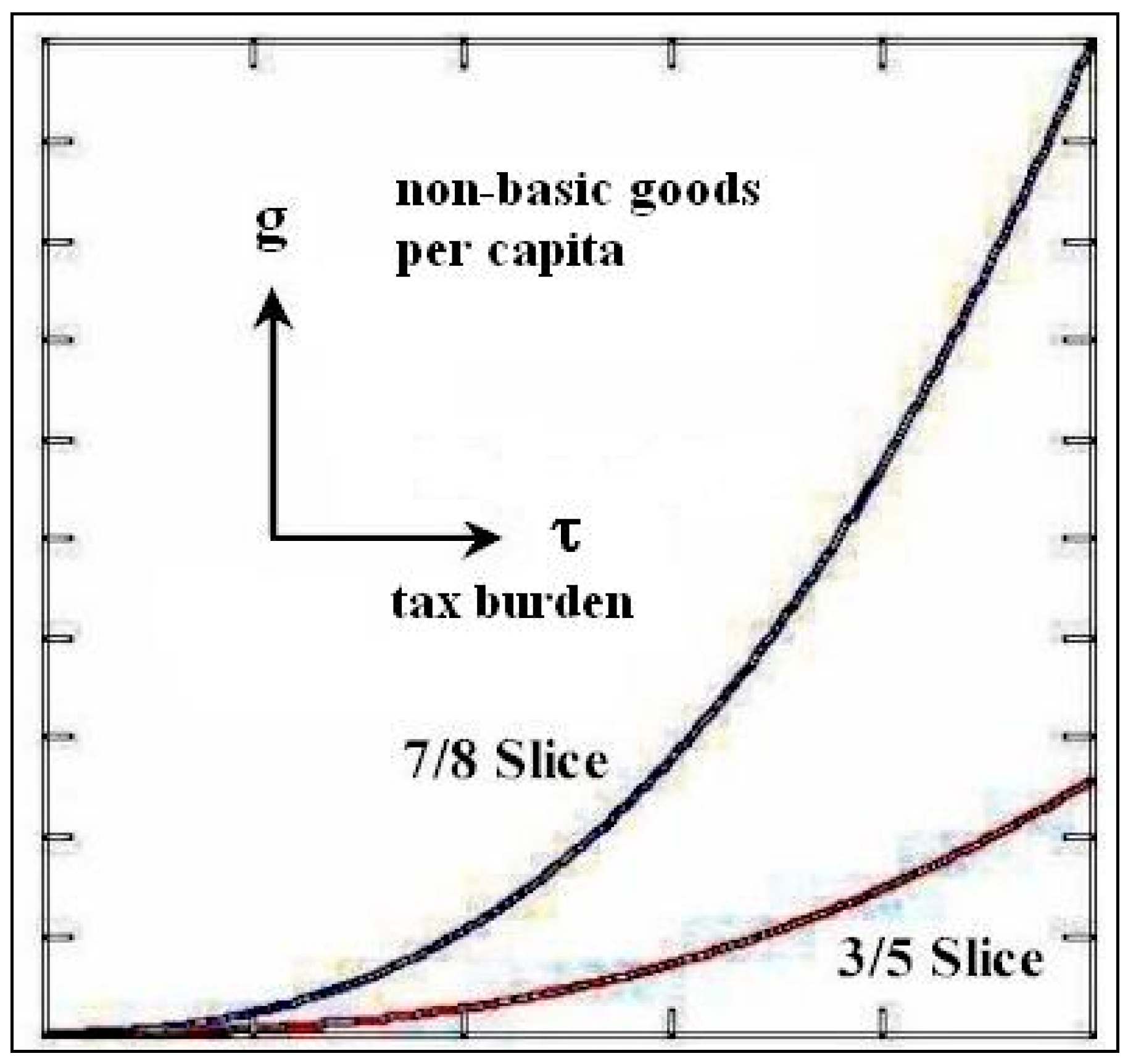
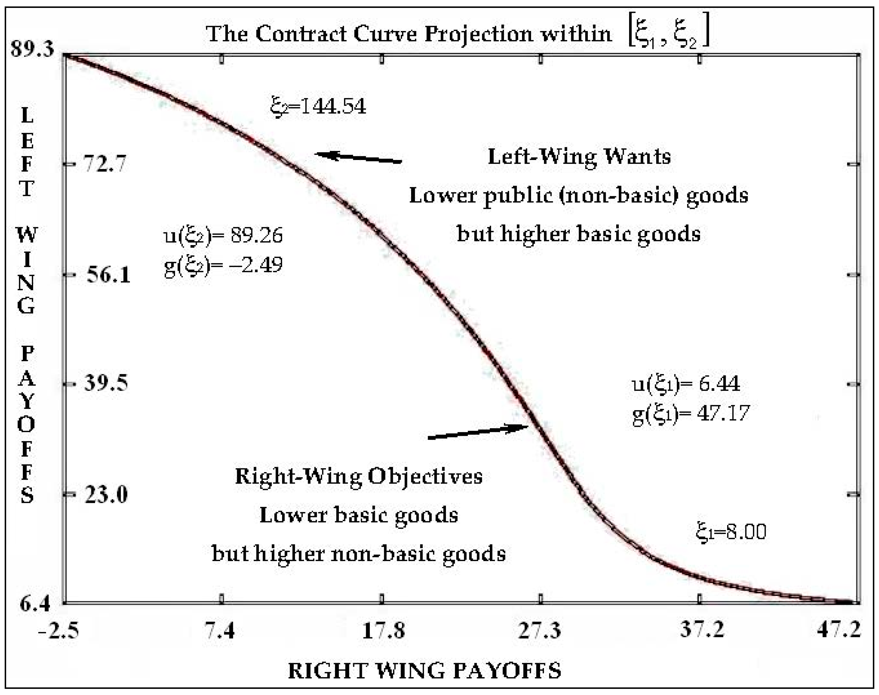