A Thermoelastic Stress Analysis General Model: Study of the Influence of Biaxial Residual Stress on Aluminium and Titanium


Abstract
:1. Introduction
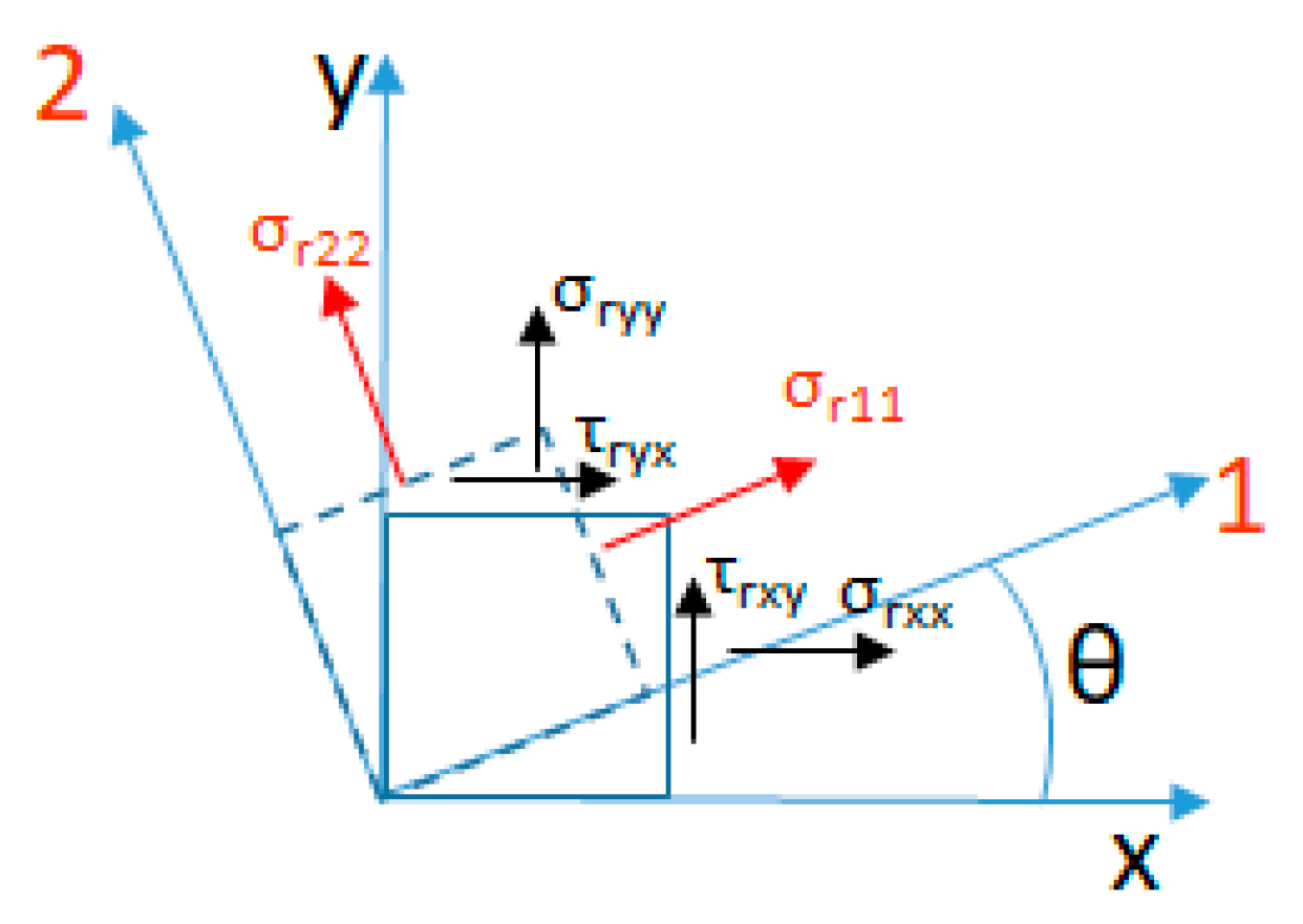
2. Theory
- The applied mean stress , here considered proportional to for each pixel in a fixed test;
- the residual stress; and
- own weight of the structure.
3. Materials and Methods
3.1. Error Analysis in Stresses Evaluation if Residual Stresses Are Neglected
3.2. TSA Capability in Evaluating Residual Stresses: Statistical Analysis
- Signal amplitude calculation (Equation (13));
- Signal temporal reconstruction, assuming a sampling frequency of 200 Hz;
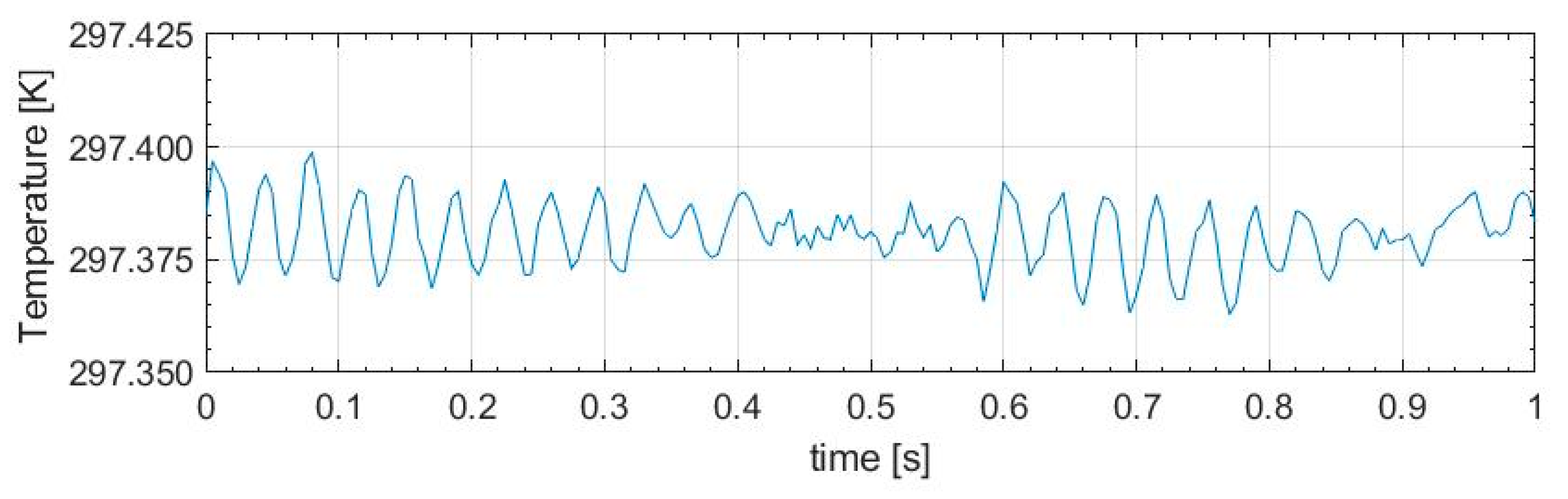
- Adding the gaussian noise according to the experimental value found with a cooled IR camera FLIR X6540sc, as described in the previous section; and
- Performing a Fast Fourier Transform to obtain the amplitude of the signal.
4. Results and Discussion
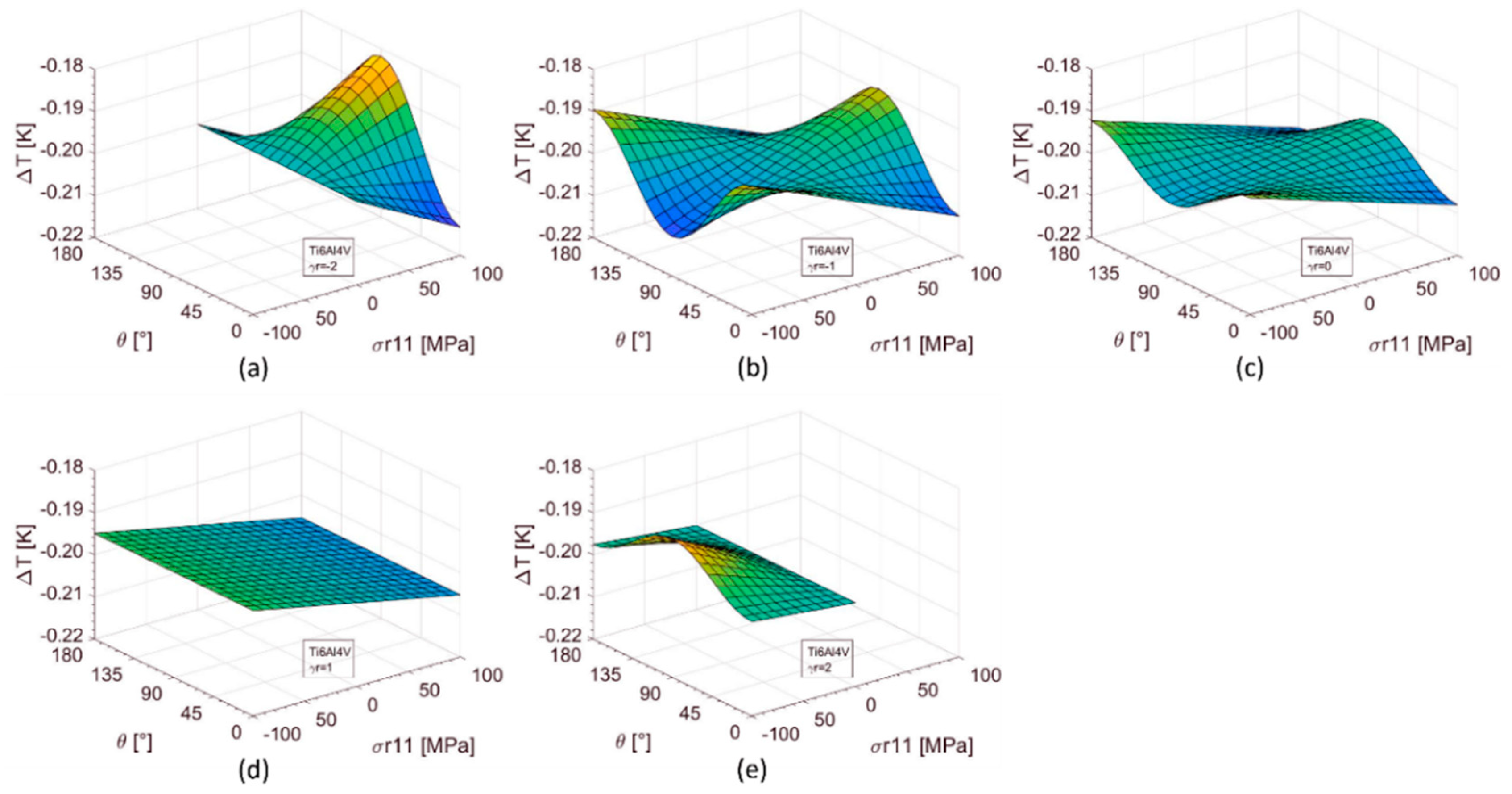
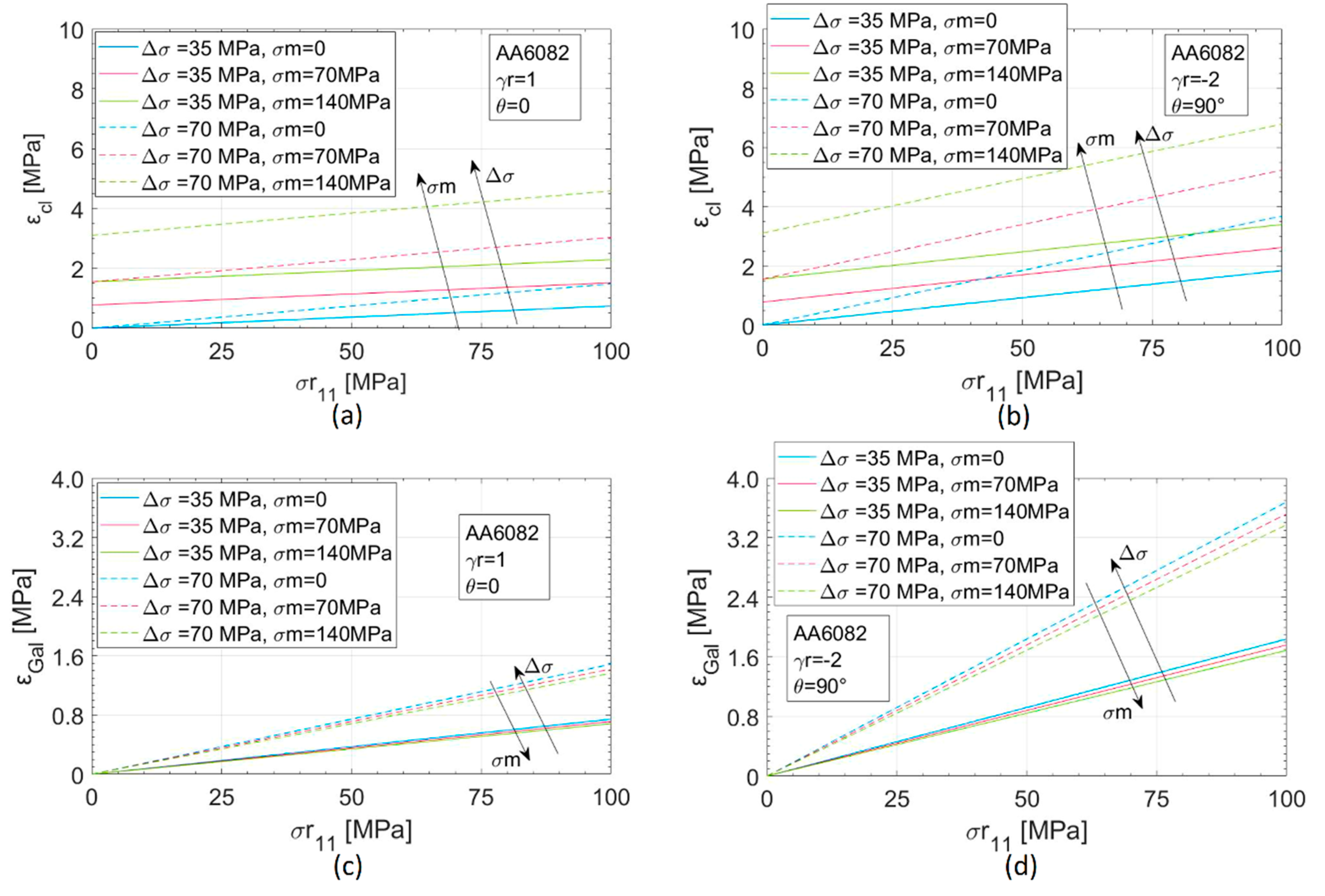
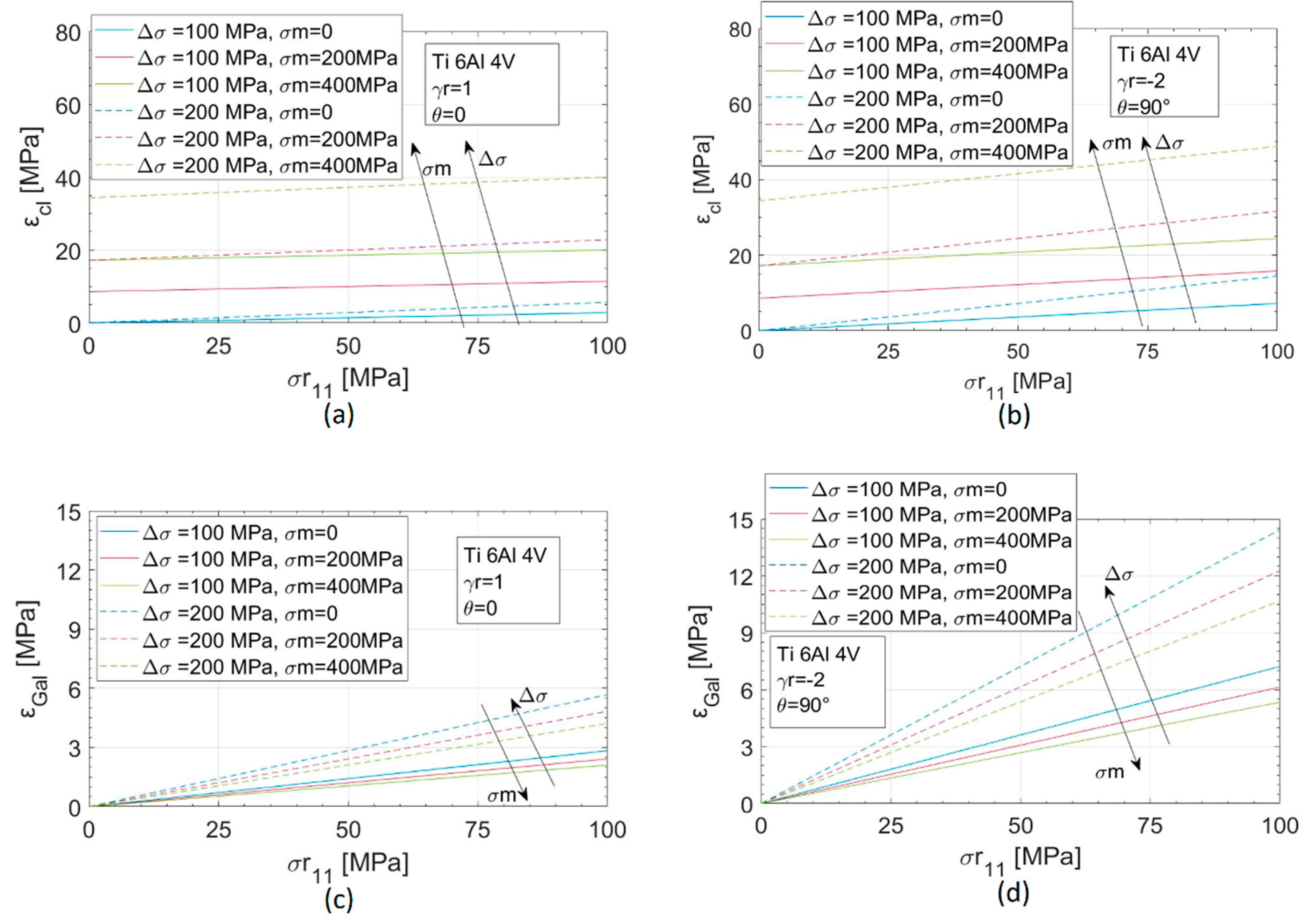
4.1. Effects of Biaxial Residual Stresses on TSA Signal
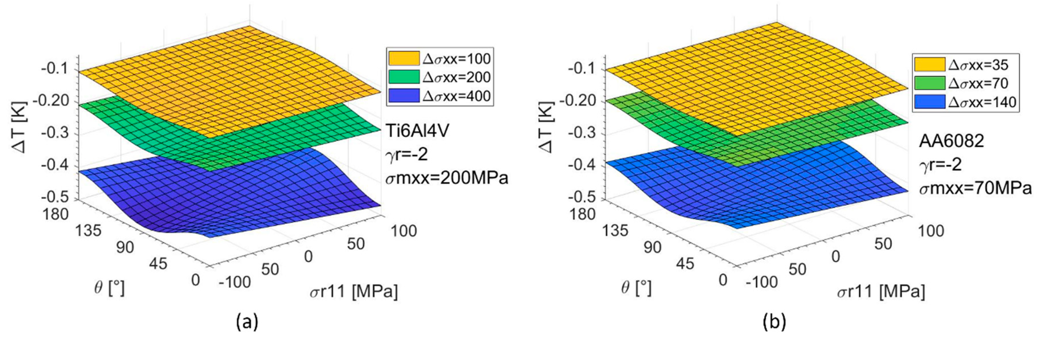
4.2. Error Analysis: Results
- The classical procedure presents the higher error;
- In the case of higher residual stress influence (γr = −2, θ = 90°), both the procedures give significant errors in stress amplitude evaluation, above 10%;
- The error increases as the stress amplitude increases for both the approaches. It is more significant for the Galietti et al. [17] approach in which the effect of the mean stress is considered; and
- The error always increases as the mean stress increases for the classic procedure while it decreases for the Galietti et al. [17] approach.
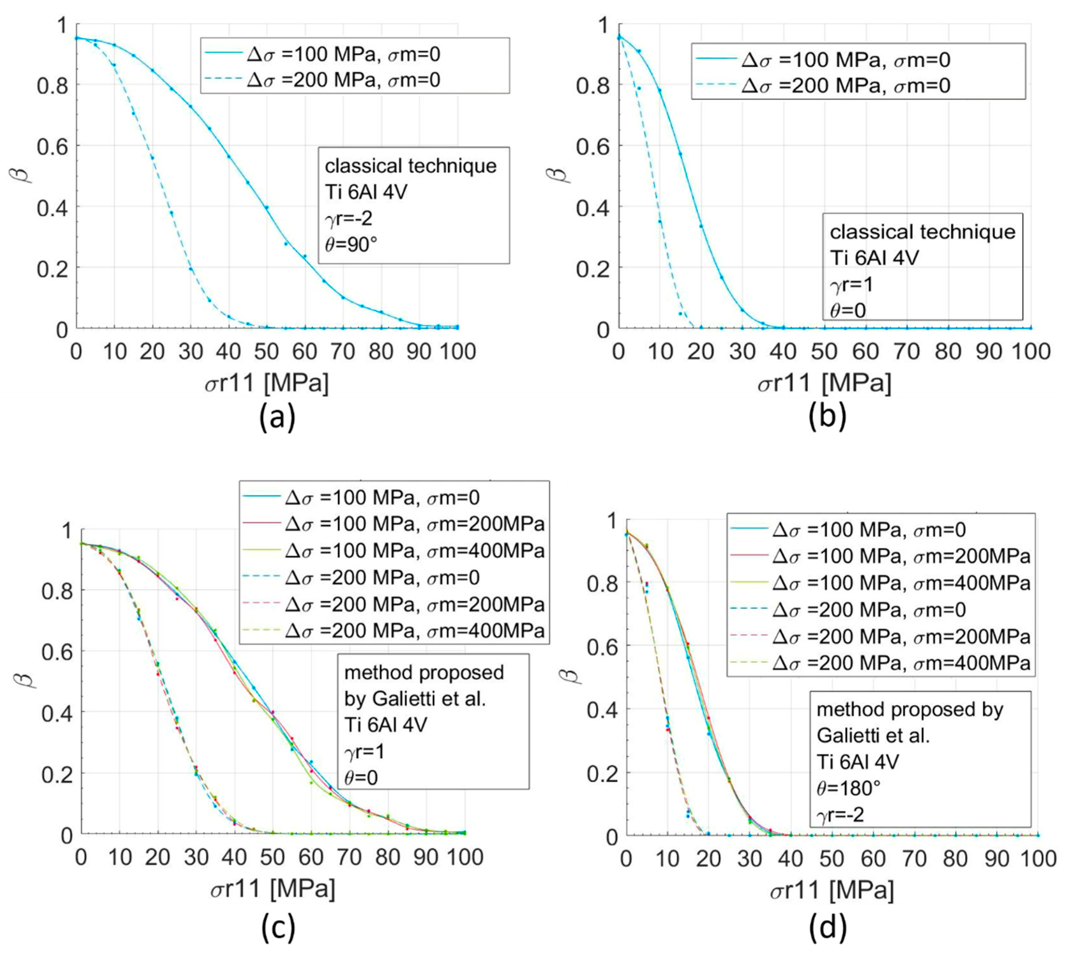
4.3. Capability in Evaluating Residual Stresses: Results
5. Conclusions
- The error in stress amplitude evaluation with TSA if the residual stresses are neglected depends on the modulus, direction and angle of the principal residual stresses with respect to the applied stresses. Significant errors (above 10%) can be made in stresses evaluation;
- This error depends also on the applied stresses (amplitude and mean) and on the considered material (thermo-physical and mechanical property); and
- In the same way, the capability of TSA in residual stresses evaluation depend on the considered material and on the modulus, direction and angle of the principal residual stresses with respect to the applied stresses.
Author Contributions
Funding
Conflicts of Interest
Nomenclature
| dT | [K] | Infinitesimal temperature difference due to the thermoelastic effect |
| T | [K] | Reference temperature |
| [μm/m] | Vector of Infinitesimal strain variations | |
| [μm/m] | Vector of strains in a point | |
| [Pa] | Stiffness matrix | |
| [K−1] | Vector of the linear thermal expansion coefficients | |
| ρ | [kg/m3] | Density |
| Cε | [J/kg·K] | Specific Heat at constant strain |
| x, y, z | - | Reference system |
| [Pa] | Vector of stress in a point | |
| [Pa] | Vector of Infinitesimal stress variations | |
| [Pa] | Amplitude stress vector | |
| [Pa] | Total mean stress vector | |
| [Pa] | Applied mean stress vector | |
| [Pa] | Residual stress vector | |
| 1,2,3 | - | Principal system |
| R | - | Rotation matrix |
| θ | - | Angle between the residual stress principal system and the loading system |
| a, b | [Pa−1], [Pa−2] | Thermoelastic parameters [16,17] |
| c | [Pa−1] | Parameter depending on thermoelastic behaviour and residual stress |
| γr | - | Ratio between the principal residual stress components |
| γ | - | Ratio between the mean and amplitude of the load |
| K | [Pa−1] | Thermoelastic constant [1] |
| ε | - | Error affecting the stress amplitude measurement |
| - | Error affecting the stress amplitude measurement using the classical technique | |
| - | Error affecting the stress amplitude measurement using the method proposed by Galietti et al. [17] | |
| β | - | Second type error |
References
- Harwood, N.; Cummings, W.M. Thermoelastic Stress Analysis; Adam Hilger: Philadelphia, PA, USA, 1991. [Google Scholar]
- De Finis, R.; Palumbo, D.; Galietti, U. A multianalysis thermography-based approach for fatigue and damage investigation of ASTM A182 F6NM steel at two stress ratios. Fatigue Fract. Eng. Mater. Struct. 2019, 42, 267–283. [Google Scholar] [CrossRef]
- De Finis, R.; Palumbo, D.; Da Silva, M.M.; Galietti, U. Is the temperature plateau of a self-heating test a robust parameter to investigate the fatigue limit of steels with thermography? Fatigue Fract. Eng. Mater. Struct. 2019, 41, 917–934. [Google Scholar] [CrossRef]
- Rajic, N.; McSwiggen, D.; McDonald, M.; Whiteley, D. In situ thermoelastic stress analysis—An improved approach to airframe structural model validation. QIRT J. 2018, 16, 8–34. [Google Scholar] [CrossRef]
- Allevi, G.; Cibeca, M.; Fioretti, R.; Marsili, R.; Montanini, R.; Rossi, G. Qualification of additively manufactured aerospace brackets: A comparison between thermoelastic stress analysis and theoretical results. Measurement 2018, 126, 252–258. [Google Scholar] [CrossRef]
- Pitarresi, G.; Patterson, E.A. A review of the general theory of thermoelastic stress analysis. J. Strain Anal. Eng. Des. 2003, 38, 405–417. [Google Scholar] [CrossRef]
- Wong, A.K.; Jones, R.; Sparrow, J.G. Thermoelastic constant or thermoelastic parameter? J. Phys. Chem. Solids 1987, 48, 749–753. [Google Scholar] [CrossRef]
- Wong, A.K.; Sparrow, J.G.; Dunn, S.A. On the revised theory of the thermoelastic effect. J. Phys. Chem. Solids 1988, 48, 395–400. [Google Scholar] [CrossRef]
- Gyekenyesi, A.L.; Baaklini, G.Y. Thermoelastic Stress Analysis: The Mean Stress Effect in Metallic Alloys. In Proceedings of the SPIE 3585, Nondestructive Evaluation of Aging Materials and Composites III, Newport Beach, CA, USA, 8 February 1999. [Google Scholar]
- Wong, A.K.; Dunn, S.A.; Sparrow, J.G. Residual stress measurement by means of the thermoelastic effect. Nature 1988, 332, 613–615. [Google Scholar] [CrossRef]
- Gyekenyesi, A.L.; Baaklini, G.Y. Quantifying Residual Stresses by Means of Thermoelastic Stress Analysis. In Proceedings of the SPIE 3993, Nondestructive Evaluation of Aging Materials and Composites IV, Newport Beach, CA, USA, 13 May 2000. [Google Scholar]
- Robinson, A.F.; Dulieu-Barton, J.M.; Quinn, S.; Burguete, L. A Review of Residual Stress Analysis using Thermoelastic Techniques. In Proceedings of the 7th International Conference on Modern Practice in Stress and Vibration Analysis, Murray Edwards College, Cambridge, UK, 8–10 September 2009; p. 012029. [Google Scholar]
- Robinson, A.F.; Dulieu-Barton, J.M.; Quinn, S.; Burguete, L. The potential for assessing residual stress using thermoelastic stress analysis: A study of cold expanded holes. Exp. Mech. 2013, 53, 299–317. [Google Scholar] [CrossRef]
- Patterson, E.A. The Potential for Quantifying Residual Stress Using Thermoelastic Stress Analysis. In Proceedings of the SEM Annual Conference and Exposition on Experimental and Applied Mechanics 2007, Springfield, MA, USA, 3–6 June 2007; pp. 664–669. [Google Scholar]
- Du, Y.; Backman, D.; Patterson, E.A. A New Approach to Measuring Surface Residual Stress Using Thermoelasticity. In Proceedings of the SEM Annual Conference and Exposition on Experimental and Applied Mechanics 2008, Orlando, FL, USA, 2–5 June 2008; Volume 2, pp. 673–680. [Google Scholar]
- Palumbo, D. Analisi Termoelastica di Componenti in Titanio e Contemporanea Valutazione Delle Tensioni Residue. In Proceedings of the Atti del XXXVIII Convegno Nazionale AIAS, Torino, Italy, 9–11 September 2009. [Google Scholar]
- Galietti, U.; Palumbo, D. Thermoelastic Stress Analysis of Titanium Components and Simultaneous Assessment of Residual Stress. In Proceedings of the EPJ Web of Conferences, ICEM 14—14th International Conference on Experimental Mechanics, Poitiers, France, 4–9 July 2010; p. 38012. [Google Scholar]
- Quinn, S.; Dulieu-Barton, J.M.; Langlands, J.M. Progress in thermoelastic residual stress measurements. Strain 2004, 40, 127–133. [Google Scholar] [CrossRef]
- Palumbo, D.; Galietti, U. Data correction for thermoelastic stress analysis on titanium components. Exp. Mech. 2016, 56, 451–462. [Google Scholar] [CrossRef]
- Potter, R.T.; Greaves, L.J. The Application of Thermoelastic Stress Analysis Techniques to Fibre Composites. In Proceedings of the SPIE 0817, Optomechanical Systems Engineering, San Diego, CA, USA, 1 January 1987. [Google Scholar]
- Fukuhara, M.; Sanpei, A. Elastic moduli and internal frictions of Inconel 718 and Ti-6Al-4V as a function of temperature. J. Mater. Sci. Lett. 1993, 12, 1112–1124. [Google Scholar] [CrossRef]
- Naimon, E.R.; Ledbetter, M.H.; Weston, W.F. Low-temperature elastic properties of four wrought and annealed aluminium alloys. J. Mater. Sci. 1975, 10, 1309–1316. [Google Scholar] [CrossRef]
- Boyer, R.; Collings, E.W.; Welsch, G. Materials Properties Handbook: Titanium Alloys; ASM International: Materials Park, OH, USA, 1994. [Google Scholar]
- ASM International. ASM Handbook Volume 2: Properties and Selection: Nonferrous Alloys and Special-Purpose Materials; ASM International: Materials Park, OH, USA, 1990. [Google Scholar]
- Benjamin, D.; Kirkpatrick, C.W. Properties and Selection: Stainless Steels, Tool Materials and Special-Purpose Metals, 9th ed.; American Society for Metals: Metals Park, OH, USA, 1980. [Google Scholar]
- Holt, H.J. Structural Alloys Handbook; West Lafayette, Ind., CINDAS/Purdue University: West Lafayette, IN, USA, 1996. [Google Scholar]
- Montgomery, D.C.; Runger, G.C. Applied Statistics and Probability for Engineers, 5th ed.; John Wiley & Sons Inc.: Hoboken, NJ, USA, 2010; p. 768. [Google Scholar]


| Material | α [K−1] | ρ [Kg/m3] | Cp [J/Kg·K] | Cε1 [J/Kg·K] | E [GPa] | υ | ∂E/∂T [MPa/K] | Rp0.2 [MPa] |
|---|---|---|---|---|---|---|---|---|
| AA6082 | 23.2 × 10⁻⁶ | 2.70 × 10³ | 890 | 890 | 70 | 0.33 | −36 | 260 |
| Ti6Al4V | 8.6 × 10⁻⁶ | 4.43 × 10³ | 560 | 560 | 114 | 0.34 | −48 | 1100 |
| Material | ∆σxx [MPa] | R | σmxx [MPa] | σr11 [MPa] | γr 1 | θ [°] |
|---|---|---|---|---|---|---|
| AA6082 | 60 | 0.1 | 73 | From −100 to 100 | From −2 to 1 | From 0 to 360 |
| Ti6Al4V | 180 | 0.1 | 220 | From −100 to 100 | From −2 to 1 | from 0 to 360 |
| Material | ∆σxx [MPa] | σmxx [MPa] | σr11 [MPa] | Residual Stresses System |
|---|---|---|---|---|
| AA6082 | 35, 70 | 0, 70, 140 | From 0 to 100 | γr = 1 and θ = 0 (low residual stresses effect) γr = −2 and θ = 90° (high residual stresses effect) |
| Ti6Al4V | 100, 200 | 0, 200, 400 | From 0 to 100 | γr = 1 and θ = 0 (low residual stresses effect) γr = −2 and θ = 90° (high residual stresses effect) |
© 2019 by the authors. Licensee MDPI, Basel, Switzerland. This article is an open access article distributed under the terms and conditions of the Creative Commons Attribution (CC BY) license (http://creativecommons.org/licenses/by/4.0/).
Share and Cite
Di Carolo, F.; De Finis, R.; Palumbo, D.; Galietti, U. A Thermoelastic Stress Analysis General Model: Study of the Influence of Biaxial Residual Stress on Aluminium and Titanium. Metals 2019, 9, 671. https://doi.org/10.3390/met9060671
Di Carolo F, De Finis R, Palumbo D, Galietti U. A Thermoelastic Stress Analysis General Model: Study of the Influence of Biaxial Residual Stress on Aluminium and Titanium. Metals. 2019; 9(6):671. https://doi.org/10.3390/met9060671
Chicago/Turabian StyleDi Carolo, Francesca, Rosa De Finis, Davide Palumbo, and Umberto Galietti. 2019. "A Thermoelastic Stress Analysis General Model: Study of the Influence of Biaxial Residual Stress on Aluminium and Titanium" Metals 9, no. 6: 671. https://doi.org/10.3390/met9060671
APA StyleDi Carolo, F., De Finis, R., Palumbo, D., & Galietti, U. (2019). A Thermoelastic Stress Analysis General Model: Study of the Influence of Biaxial Residual Stress on Aluminium and Titanium. Metals, 9(6), 671. https://doi.org/10.3390/met9060671