Prediction of Wrinkling of a Beverage Can Subjected to the Redrawing Process by J2 Deformation Theory

Abstract

Wrinkling of beverage cans is one of the problems faced by can manufacturers and aluminum suppliers. The bottom of an aluminum can is wrinkled by compression during the forming process. In this study, to predict the occurrence of wrinkles during the redrawing process of AA3104 (t = 0.265 mm), which is the material used to fabricate aluminum cans, the classical plasticity J2 deformation theory (J₂D) and flow theory (J₂F) were considered. J₂F considers only the deformation perpendicular to the yield locus, whereas J₂D considers the deformation perpendicular to the yield locus and that tangential to the yield locus. Wrinkles are predicted using finite element (FE) analyses based on J₂D and J₂F, and the results are compared. J₂F could not predict the number and amplitude of wrinkles. By contrast, the wrinkles predicted using J₂D exhibited good agreement with sample data obtained for a real can. To find the difference between the results obtained using J₂F and J₂D, evolutions of stress path in a wrinkled element are compared. It was confirmed that compressive stress is more dominant in the J₂D case than in the J₂F case. Moreover, the measured effective strain of the element is small, under 0.04. In conclusion, J₂D is more suitable for predicting the wrinkling behavior of aluminum cans than J₂F. In addition, ANOVA and ANOM analysis are performed to evaluate the influence of the design parameters, namely friction coefficient, thickness, and outer profile angle, and the parameters are optimized to reduce wrinkles by combining the Taguchi method with FE simulation based on the J₂D theory.

1. Introduction

Wrinkling problem is encountered in the drawing of automotive parts and beverage cans for over 40 years. A known cause of wrinkles is compressive stress due to plastic behavior during the formation of thin sheets. Indeed, the aluminum manufacturers, can makers manufacturing techniques and cost control efforts have resulted in thinner sheet thicknesses, thereby causing wrinkle problems. To avoid wrinkling and obtain the desired shape, the effect of the blank holding force, clearance between punch and lower die, tool design, and lubrication have been studied. When the blank holding force is increased to reduce wrinkling, problems, such as thinning and fracture of the sheet, should be considered. In addition, wrinkling is affected by many factors, such as material properties and thickness, and tool geometry, such as outer profile angle, coefficient of friction, and lubrication. Especially, these factors are more sensitive in the case of beverage cans because the blank is very thin, ranging from 0.2 to 0.4 mm. Moreover, the process of aluminum beverage can is consists of drawing and ironing (D&I). The wrinkles in the beverage can are known to occur during the redrawing process.

Figure 1 shows a schematic diagram of the process to fabricate beverage cans. The occurrence of wrinkles on the bottom of the beverage can is shown in Figure 2. In the same figure, many small wrinkles can be observed. To overcome such wrinkling, optimization approaches have been investigated in previous studies [1,2,3]. Moreover, process designers and engineers are expanding the application of finite element (FE) simulations [4,5]. FE simulations have been used to predict wrinkling for more than 30 years now [6,7,8,9,10,11]. Cao et al. [12,13,14,15] employed FE simulation to predict wrinkling behavior in sheet metal forming. Makinouchi [16] conducted FE simulations to study the effect of blank holding on wrinkling in automotive parts. Nam and Han [17] studied the anisotropic effects of low-carbon steel sheets by comparing their thickness distributions after D&I. Rekas [18] studied the effect of the thickness of AA3XXX grade sheet on wrinkling by performing an FE simulation. The author identified the optimum sheet thickness for obtaining a good product given that the proper tool geometry, process parameters, and clearance are selected. Kawka et al. [19] predicted the wrinkles formed after deep drawing. They considered plastic behaviors by using the hardening function and the anisotropic yield function to describe material properties accurately. Kim and Son [20] approached wrinkling in terms of various material parameters, such as yield stress, hardening coefficient, and perpendicular anisotropy. They reported that wrinkles are formed rapidly as the hardening exponent n decreases, initial yield stress increases, and thickness decreases. Moreover, they investigated the wrinkle limits numerically. Recently, the wrinkle prediction problem was presented as a benchmark at NUMISHEET 2014. Kim et al. [21] predicted the onset and growth of wrinkles by adopting a bifurcation algorithm to implement cylindrical cup deep drawing. Most researchers have pointed out that tool path, die, blank holder, heating condition, friction, and appropriate material properties must be considered simultaneously to obtain accurate FE simulation results.

Under the classical plasticity theory, two theories have been developed to calculate strain, namely flow theory and deformation theory. The two theories differ in the manners in which they compute strain rate. Flow theory has been used widely because it consists of simple governing equation terms and it is easy to implement in FE simulation programs. Hutchinson et al. [22,23,24,25,26] studied and compared deformation theory and flow theory by using the von Mises yield function based on an invariant J2. Cao et al. [27] showed that a wide range of material characteristics can be applied by implementing FE simulation based on the kinematic-hardening model and the J2 flow theory (J₂F) or J2 deformation theory (J₂D).

Neale and Hassani [28] reported the influences of J₂D and J₂F on the wrinkling limit diagram of an isotropic material. They found that the deformation theory of plasticity predicted wrinkling at lower stress levels than the flow theory, as expected, and the deformation theory generated more conservative predictions of the onset of wrinkling.

Dick and Yoon [29] studied the effects of the hardening function and anisotropic yield function from the viewpoint of considering the properties of anisotropic material behavior. Moreover, they performed an FE simulation by using the flow theory in conjunction with Barlat’s Yld2000-2d anisotropic yield function [30], which provides a good description of anisotropic material behavior. To evaluate the hardening effect, they considered four different hardening curves of AA 5042 and compared wrinkling behaviors, punch forces, and punch displacements. The comparison results indicated that a lower yield stress significantly reduced the magnitude of wrinkling. Although the predicted punch force was higher than the experimental value, the results obtained using the four different hardening curves were almost identical. Moreover, the results of the simulation performed using the Yld2000-2d anisotropic yield function agreed well with the experimental results. The magnitude of the wrinkles was larger than 2 mm and the number of wrinkles was small, that is 13 wrinkles over 360°.

In this study, we considered beverage cans because more than 40 wrinkles of small magnitude are created in the fabrication of this product. We performed FE simulations based on the classical plasticity theories of J₂D and J₂F to predict the occurrence of wrinkles. Moreover, we considered only the redrawing process because wrinkles are formed in this process. According to this consideration, the blank was assumed to have a homogeneous thickness of 0.265 mm because this thickness is obtained after deep drawing in a real process. To perform the FE simulation, commercial software ABAQUS/STANDARD was used for wrinkle prediction. In addition, Taguchi’s orthogonal array simulations were combined with the FE simulations to quantify and optimize the main variables affecting the forming quality of a can. Three design variables, namely friction coefficient, blank thickness, and outer profile angle, were optimized. The simulation results obtained using the optimized variables indicated reduced wrinkle formation.

2. Classical Plasticity Theory

2.1. J2 Deformation Theory

Storen and Rice [31] proposed the J2 deformation theory based on the necking phenomenon, which is a local plastic deformation caused by the instability of plane stresses. This theory was derived by assuming a local bifurcation by using the difference in the velocity rates of deformation between the interior and exterior sides of a thin sheet. In J₂D, the hypothesis is initial isotropic in plastic behavior and plastic deformation covers only changes in shape, not changes in volume. The second invariant J2 was employed as the isotropic yield function, commonly called the von Mises yield function. The yield function can be expressed as follows:

$${\sigma }_{VM}=\sqrt{\frac{1}{2}\left[{\left({\sigma }_1-{\sigma }_2\right)}^2+{\left({\sigma }_2-{\sigma }_3\right)}^2+{\left({\sigma }_3-{\sigma }_1\right)}^2\right]}$$

(1)

where ${\sigma }_1$, ${\sigma }_2$, and ${\sigma }_3$ denote the principal stresses. In the case of plane stress, the above function can be simplified as follows:

$${\sigma }_{VM}=\sqrt{{\sigma }_1^2-{\sigma }_1{\sigma }_2+{\sigma }_2^2}$$

(2)

J₂D can be expressed in terms of equivalent stress ($\overline{\sigma }$) and equivalent plastic strain (${\overline{\epsilon }}^p$). The equivalent stress and equivalent plastic strain can be written as follows:

$$\overline{\sigma }=\sqrt{\left(3/2\right){\sigma }_{ij}^{\prime }{\sigma }_{ij}^{\prime }},{\overline{\epsilon }}^p=\sqrt{\left(2/3\right){\epsilon }_{ij}^p{\epsilon }_{ij}^p}(\mathrm{i},\mathrm{j}=1,2)$$

(3)

here ${\sigma }_{ij}^{\prime }$ and ${\epsilon }_{ij}^p$ denote the deviatoric stress and plastic strain tensor, respectively. By using Hencky’s equation, one can express the plastic strain (${\epsilon }_{ij}^p$) as follows:

$${\epsilon }_{ij}^p={\sigma }_{ij}^{\prime }\varnothing$$

(4)

and

$$\varnothing =\frac{3}{2}\frac{{\overline{\epsilon }}^p}{\overline{\sigma }}=\frac{3}{2}\frac{\overline{\epsilon }-{\overline{\epsilon }}^e}{\overline{\sigma }}=\frac{3}{2}\left(\frac{1}{E_s}-\frac{1}{E}\right)$$

(5)

where $\varnothing$ and ${\overline{\epsilon }}^p$ denote a proportional constant and the plastic equivalent strain, respectively. Moreover, the plastic equivalent strain can be rewritten in terms of total strain ($d\overline{\epsilon }$) and elastic strain ($d{\overline{\epsilon }}^e)$. $E_s$ $\left(=\frac{\overline{\sigma }}{\overline{\epsilon }}\right)$ and E $\left(=\frac{\overline{\sigma }}{{\overline{\epsilon }}^e}\right)$ denote the secant modulus and modulus of elasticity obtained from the stress-strain curve, respectively.

Using the above equation, one can express the derivative term ($\dot{\varnothing }$) of the proportional constant ($\varnothing$) as follows:

$$\dot{\varnothing }=\frac{3}{2}\frac{\dot{\overline{\sigma }}}{\overline{\sigma }}\left(\frac{1}{E_t}-\frac{1}{E_s}\right)$$

(6)

where $E_t$ denotes the tangential modulus of elasticity, and $\dot{\overline{\sigma }}$ represents the velocity for equivalent stress. The velocity of plastic strain (${\epsilon }_{ij}^p$) in Equation (4) can be written as follows:

$${\dot{\epsilon }}_{ij}^p=\frac{3}{2}\left(\frac{1}{E_s}-\frac{1}{E}\right){\dot{\sigma }}_{ij}^{\prime }+\frac{9}{4}\left(\frac{1}{E_t}-\frac{1}{E_s}\right)\frac{{\sigma }_{ij}^{\prime }{\sigma }_{kl}^{\prime }}{{\overline{\sigma }}^2}{\dot{\sigma }}_{kl}^{\prime }$$

(7)

This equation can be expressed simply by substituting A and B as follows:

$${\dot{\epsilon }}_{ij}^p=A{\dot{\sigma }}_{ij}^{\prime }+B\frac{{\sigma }_{ij}^{\prime }{\sigma }_{kl}^{\prime }}{{\overline{\sigma }}^2}{\dot{\sigma }}_{kl}^{\prime }$$

(8)

where A = $\frac{3}{2}\left(\frac{1}{E_s}-\frac{1}{E}\right)$ and B = $\frac{9}{4}\left(\frac{1}{E_t}-\frac{1}{E_s}\right)$. Equation (8) is the mathematical expression of the deformation theory.

In the above equation, the first and second terms on the right-hand side of Equation (8) describe the plastic deformation in the vertical direction and the tangential direction from the yield locus, respectively. In contrast to J₂F, which assumes that plastic deformation occurs only perpendicular to the yield locus, J₂D permits deformation in both the vertical and tangential directions. This can be confirmed from Equation (8).

2.2. J2 Flow Theory

J₂F, too, uses an isotropic yield function based on the second invariant J2. In Equation (8), when $E_s=E$, A = 0 and B = $\frac{9}{4}\left(\frac{1}{E_t}-\frac{1}{E}\right)$. Therefore, Equation (8) becomes the equation for J₂F and it can be expressed as follows:

$${\dot{\epsilon }}_{ij,F}^p=\frac{9}{4}\left(\frac{1}{E_t}-\frac{1}{E}\right)\frac{{\sigma }_{ij}^{\prime }{\sigma }_{kl}^{\prime }}{{\overline{\sigma }}^2}{\dot{\sigma }}_{kl}^{\prime }$$

(9)

From the above equation, it can be confirmed that J₂F considers plastic deformation only in the perpendicular direction.

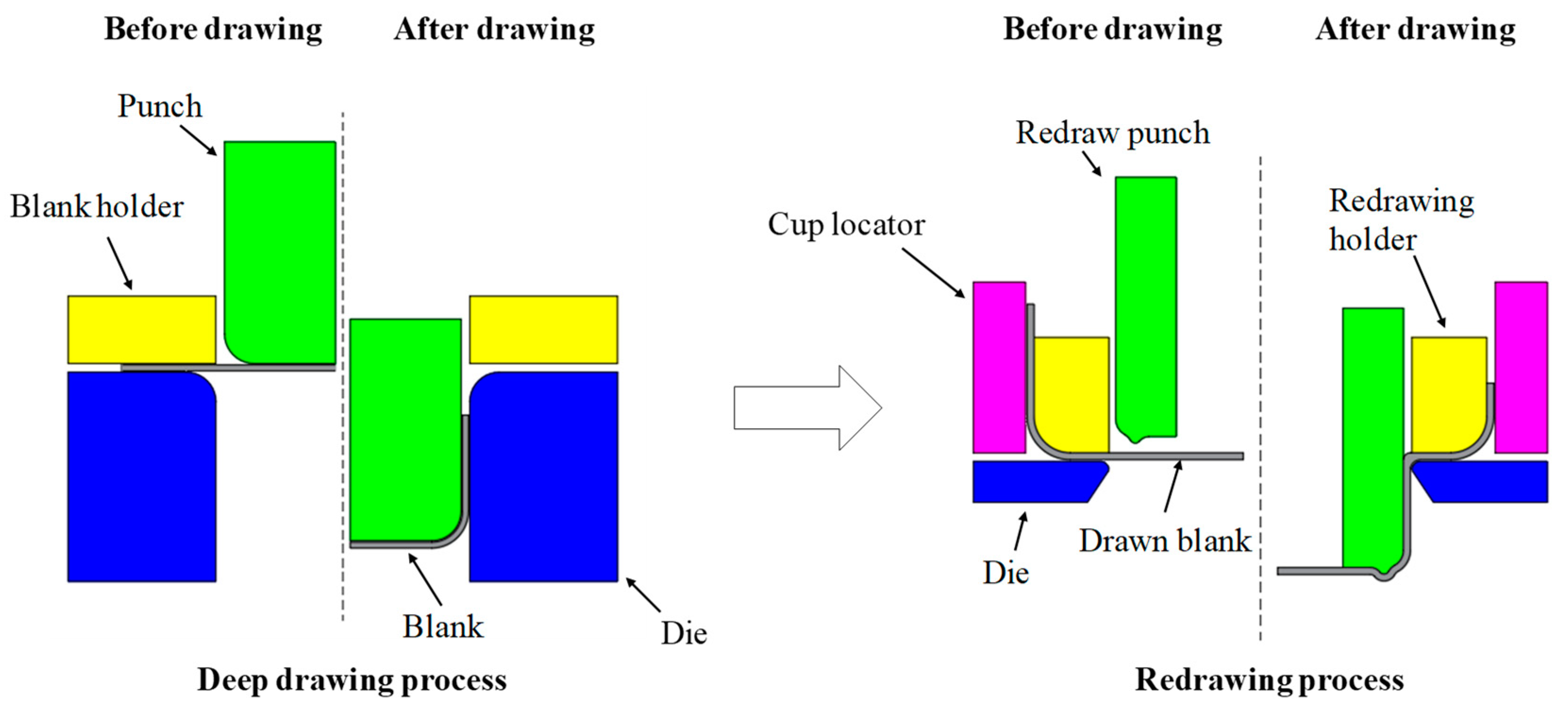
3. Experiment and Finite Element Models

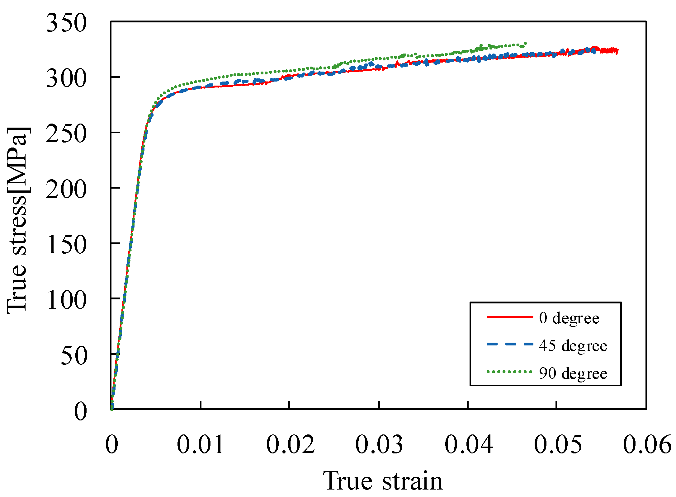
3.1. Uniaxial Tensile Test

To confirm the flow stress-strain relationship and the anisotropic behavior of an AA3104 sheet, uniaxial tensile tests were performed at θ = 0°, 45°, and 90° relative to the rolling direction (RD). Specimens were prepared using a laser machine according to the ASTM-E8 standard. The tensile tests were carried out at a strain rate of approximately 1 mm/min. The initial yield stress and r-value were measured in the same test.

Figure 3 shows the true stress-strain curves at θ = 0°, 45°, and 90° relative to the RD. In the figure, the results of the tensile test depict isotropic material behavior, but the r-values (0°: 0.41, 45°: 0.99, and 90°: 1.02) indicate anisotropic material behavior. The mechanical properties obtained from the uniaxial tension test are summarized in

Table 1. Mechanical properties of AA3104 sheet.

Test Direction	E (GPa)	υ	UTS (MPa)	YS (MPa)	r-Value
0°	69.73	0.33	310.5	281	0.41
45°	69.24	0.32	308.8	280	0.99
90°	69.41	0.33	316.8	286	1.02

, including modulus of elasticity (E), Poisson’s ratio (υ), ultimate tensile strength (UTS), initial yield stress (YS), and r-values.

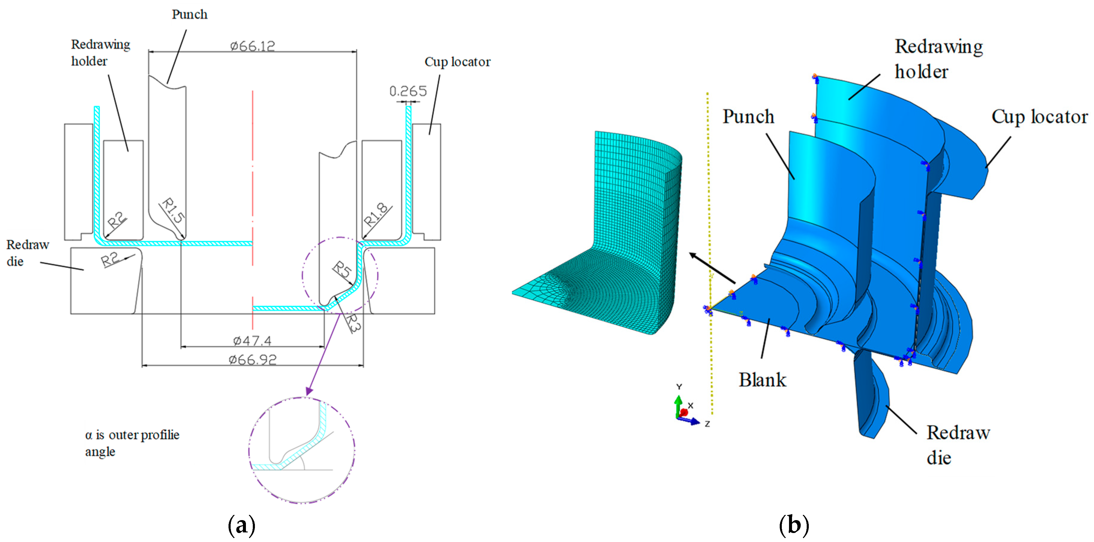
3.2. Geometrical Model

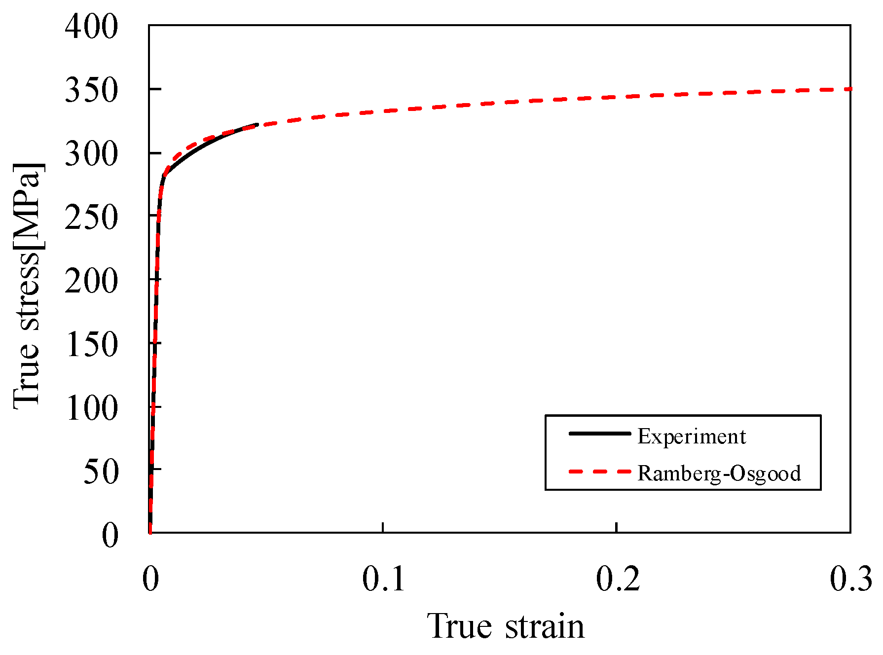
Can manufacturing involves multiple deep drawing processes, including redrawing, three-step ironing, doming, trimming, and flanging. However, because wrinkles occur during redrawing, only the redrawing process was considered for wrinkle prediction. A schematic drawing of the redrawing process and the corresponding geometry for FE simulation along with a mesh of the blank are shown in Figure 4a,b, respectively. The FE simulation model consisted of a redraw die, blank holder, punch, cup locator, and blank with 1/4 symmetry. The tool and can dimensions were set by referencing the size of a commercially manufactured 12-oz (355 mL) D&I can [18,19]. In addition, the external profile angle was modeled as α = 37°. The redraw die and punch were set as a rigid body for analysis. The four-node shell element (S4R) and five integration points in the thickness direction were applied and the smallest element size of the blank was set to 1 mm × 0.9 mm. A blank holding force of approximately 11 kN was applied. Moreover, the friction coefficient between all parts (the blank holder and the plate, the punch and the plate, the cup locator and the blank) was applied in the form of penalty friction coefficient of 0.05 since the range of that is from 0.03 to 0.07 for a real can making process [17,29,32]. The punch stroke was set to be 13.5 mm from contact to the final step.

3.3. Material Model

FE simulations based on J₂F and J₂D were performed using commercial software ABAQUS/STANDARD. To describe the material behavior during the redrawing process, the Ramberg–Osgood [33] plasticity model was adopted to represent the flow stress of AA3104 material in the FE simulation. A one-dimensional model of this equation can be expressed as follows:

$$\mathsf{\epsilon }=\frac{\mathsf{\sigma }}{E}+K{\left(\frac{\mathsf{\sigma }}{E}\right)}^n$$

(10)

where E, ε, σ, K and n are elastic modulus, strain, stress, material constant, and hardening exponent, respectively. By introducing the yield strength of the material, ${\sigma }_0$, and defining a new parameter, α, related to K as $\alpha =K{\left({\sigma }_0/E\right)}^{n-1}$, the Equation (10) can be rewritten as follows:

$$E\epsilon =\sigma +\alpha {\left(\frac{\left|\sigma \right|}{{\sigma }_0}\right)}^{n-1}\sigma$$

(11)

here, E = 69.73 GPa, ${\sigma }_0$ = 281 MPa, α = 0.45, and n = 22.59 were applied to explain the flow curve of AA3104. The curve obtained using Equation (11) and experimental data (0°) are shown in Figure 5. The result of the fitting curve shows that the Ramberg–Osgood model can describe the experiment well.

4. Results and Discussions

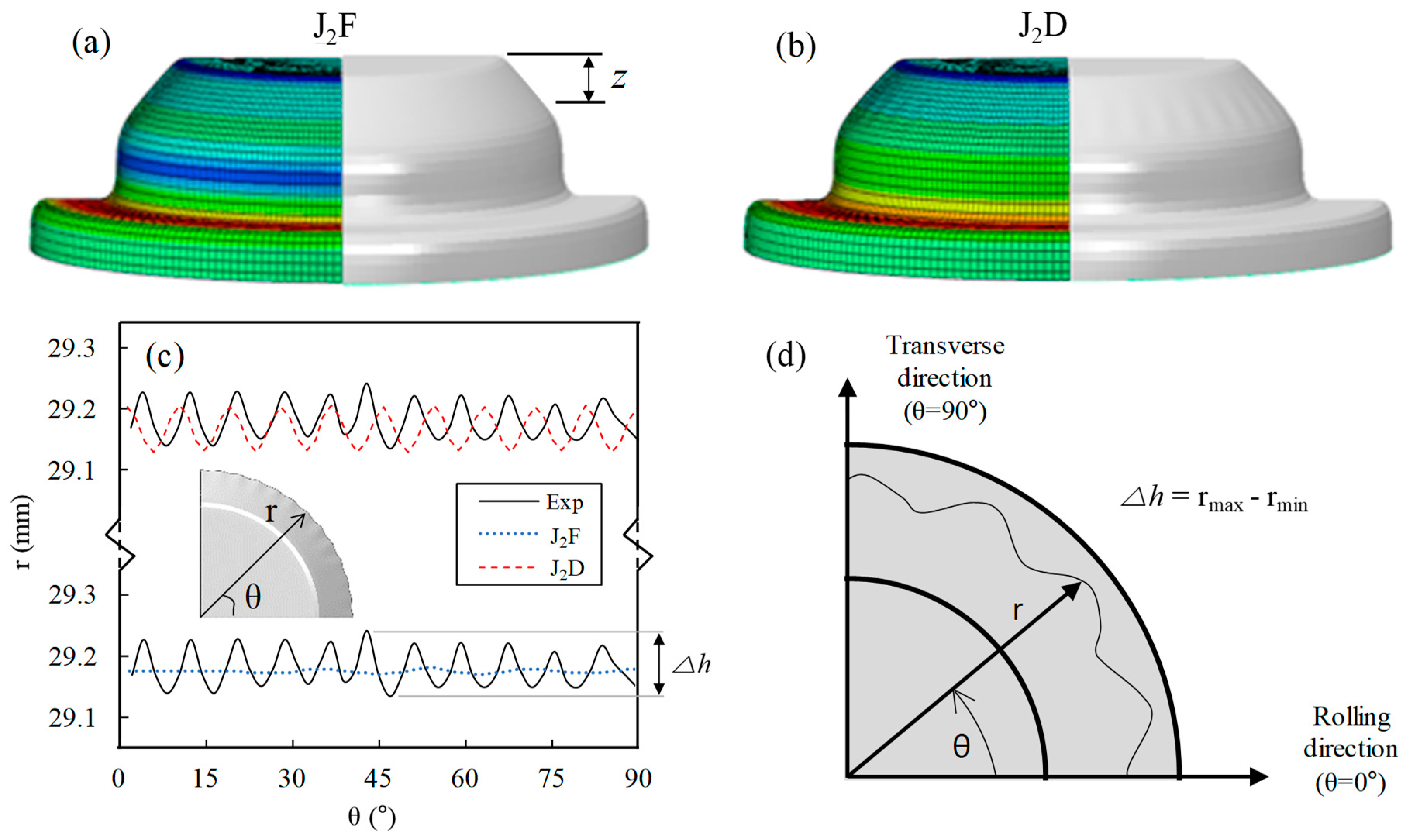
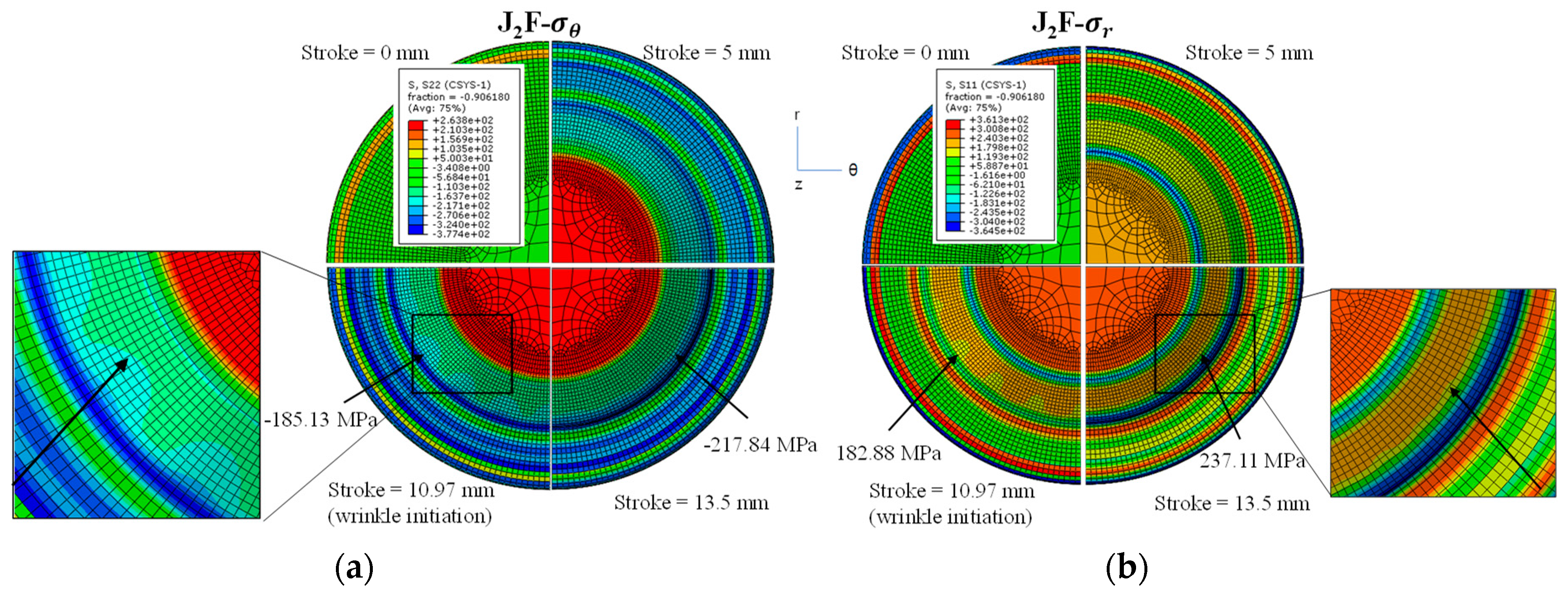
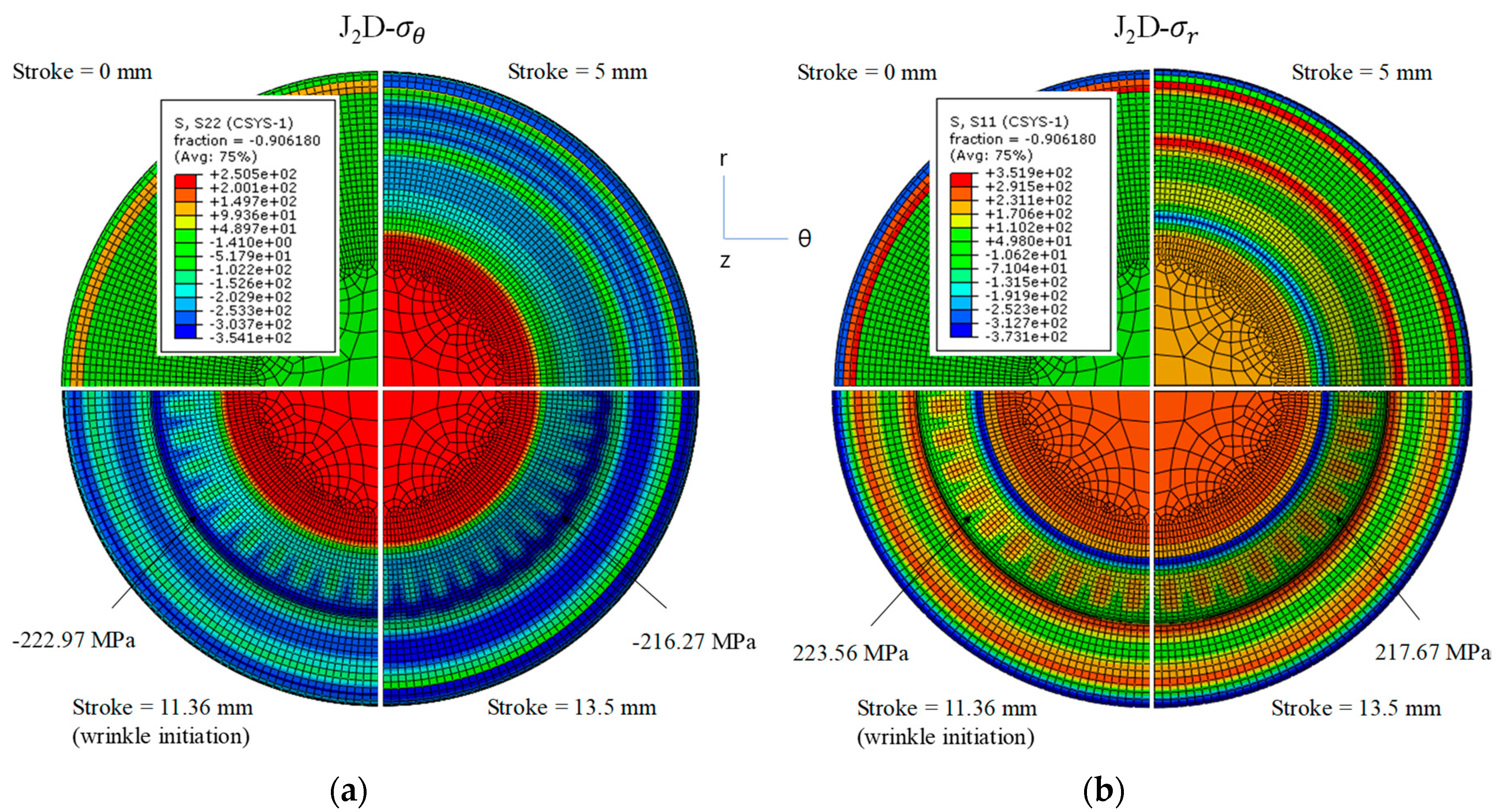
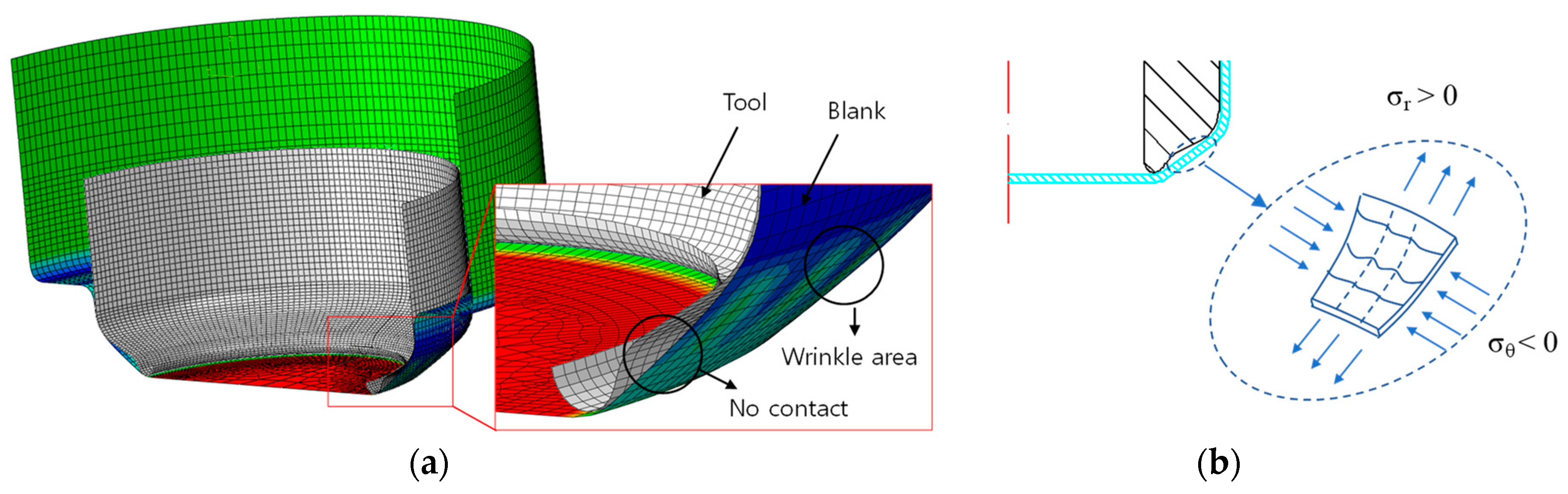
4.1. Wrinkling Prediction

The strain distribution at the final stage was analyzed with both J₂F and J₂D, as shown in Figure 6a,b, respectively. In this figure, the strain distribution is uniform along the radial direction because it is based on the second invariant J2. In addition, the wrinkled sample used in this study was obtained from a can manufacturer and the wrinkles were measured at z = 3.5 mm from the bottom of the can because the maximum wrinkling was observed at this point. To compare the wrinkles indicated by each theory and the actual wrinkles on the sample can, the radial distance was measured at the same position (z = 3.5 mm) on the sample can (Figure 6c). A schematic diagram of the wrinkle measurement process is illustrated in Figure 6d. $\Delta h$ denotes the highest wrinkle amplitude and can be obtained from $\Delta h=r_{max}-r_{min}$. Only one sample was used since the characteristics, which are amplitudes and the number of wrinkles, are similar in most samples. During experimental processes, only one ∆h was determined for one sample and each FE model also provided just one value of $\Delta h$. In this study, the value of $\Delta h$ was determined directly from the measurement without any deviation because the wrinkles were measured for only one sample.

Eleven wrinkles were observed on the sample obtained from the manufacturer. However, four wrinkles were predicted in the simulation based on J₂F, while 10 wrinkles were predicted in the simulation based on J₂D. The $\Delta h$, which means the maximum value of amplitudes measured on the sample can, was approximately 0.108 mm and the simulations based on J₂F and J₂D yielded $\Delta h$ predictions of approximately 0.009 mm and 0.077 mm, respectively.

To identify the evolution of the stress path at the point of wrinkle occurrence, the stress path obtained from an element in which wrinkles occurred and the initial von Mises yield locus are shown in Figure 7. The circle represents the initial yield locus, and the solid and dotted lines show the stress paths obtained in the simulations based on J₂D and J₂F, respectively. In addition, the pure shear line is shown to confirm the dominance of the compressive stress region, where the left side of the pure shear line is predominant. Both stress paths are similar in the elastic region. However, in the plastic region, the stress path measured from J₂F is shifted to the upper of the pure shear line (second quadrant), while that obtained from J₂D is shifted toward the left of the pure shear line (second quadrant). This means that the stress path of J₂D is in the region dominated by compressive stress compared to that of J₂F. Because wrinkle formation is dominated by compressive stress, the prediction obtained using J₂F is superior to that obtained using J₂D. This result is consistent with the results of previous studies, which indicate that wrinkle formation is governed by compressive stress. The magnitudes of stresses and strains for both cases in the final stroke (13.5 mm) were measured: ${\sigma }_{11}$ = −126 MPa, ${\sigma }_{22}$ = 199.8 MPa and ${\mathsf{\epsilon }}_{11}$ = −0.027, ${\mathsf{\epsilon }}_{22}$ = 0.026 for J₂F and ${\sigma }_{11}$ = −248.0 MPa, ${\sigma }_{22}$ = 83.8 MPa and ${\mathsf{\epsilon }}_{11}$ = −0.034, ${\mathsf{\epsilon }}_{22}$ = 0.024 for J₂D. Moreover, the stress and strain values indicate that J₂D is in the area of plastic behavior, where compression is predominant.

To verify the wrinkling behavior, the stresses at a cylindrical coordinate, which uses the radial, circular, and axial directions, were analyzed for J₂F and J₂D. Figure 8 and Figure 9 show the predictions of stress distributions on the outer surface of the deformed specimen based on the J₂F and J₂D theories, respectively. Both figures indicate a negative value of ${\sigma }_{\mathsf{\theta }}$ and positive value of ${\sigma }_{\mathrm{r}}$. In other words, the material was stretched in the radial direction and compressed in the circular direction, which can be seen in the figures. The stress distributions were measured at punch stroke = 0, 5, wrinkle initiation stroke, and final stroke. In both figures, the punch strokes of 0 and 5 mm did not lead to wrinkle formation, while the wrinkle initiation stroke (10.97 mm for J₂F and 11.36 mm for J₂D) and the final stroke led to stress distributions with wrinkle formation. However, J₂F predicted the formation of a small number of wrinkles, whereas J₂D predicted the formation of a large number of wrinkles. Moreover, the stretched stress and compressive stress at the initiation stroke were more dominant according to J₂D than J₂F, but those of them in the final stroke show converse results. The radial stress in the final stroke was more dominant according to J₂F than J₂D. The stresses at the initiation stroke and final stroke were as follows: J₂F (${\sigma }_{\mathsf{\theta }}$ = −185.13 MPa, ${\sigma }_{\mathrm{r}}$ = 182.88 MPa for wrinkle initiation, and ${\sigma }_{\mathsf{\theta }}$ = −217.84 MPa, ${\sigma }_{\mathrm{r}}$ = 237.11 MPa for final stroke); J₂D (${\sigma }_{\mathsf{\theta }}$ = −222.97 MPa, ${\sigma }_{\mathrm{r}}$ = 223.56 MPa for wrinkle initiation and ${\sigma }_{\mathsf{\theta }}$ = −216.27 MPa, ${\sigma }_{\mathrm{r}}$ = 217.67 MPa for final stroke), respectively. These results are consistent with the results of Neale and Tugcu [28]. Moreover, the difference between global and cylindrical coordinate system stresses comes from coordinate systems.

To identify the cause of wrinkle occurrence, we observed the contact region between the tool and the blank. Figure 10a shows the redrawing tool and blank of half of the model. In the figure, the tool is not contacting the blank in the wrinkled area during redrawing. It is easy to apply compressive stress to the blank. Because of this phenomenon, the blank is wrinkled easily. Moreover, the stress mode of a wrinkled element is illustrated in Figure 10b to depict the wrinkling mechanism. On the cylindrical coordinates, the element is subjected to tensile stress along the radial direction ®, which is indicative of the drawing mode. In contrast, it is subjected to compressive stress along the angle direction (θ). Wrinkles are easily generated in this mode. Because wrinkles are formed according to this mechanism, the outer profile angle, which affects to condition of contact, is an important design parameter. Moreover, to confirm the strain value at the element in which wrinkling occurred, the effective strains according to the punch stroke were determined using the J₂D and J₂F theories and compared with each other (Figure 11). Both strains were less than 0.04. This result indicated that a small deformation occurred in the wrinkled area. Based on the above observations, J₂D is more suitable for wrinkle prediction than J₂F.

4.2. Wrinkle Optimization

In the light of the above observations, Taguchi’s orthogonal arrays were employed in conjunction with FE simulation based on J₂D to optimize the redrawing process conditions to avoid wrinkle formation. In a Taguchi orthogonal array experiment, the objective function to be optimized must be defined. Moreover, the signal-to-noise (S/N) ratio, a higher value of which indicates a superior result, was used. The S/N ratio is defined as follows:

$${\eta }_i=-10\log \left(\Delta h_i^2\right),$$

(12)

where η_i and ∆h_i are the observed value (in dB) and the highest amplitude at z = 3.5 mm from the bottom of the can in the i-th simulation, respectively. The highest value of the S/N ratio corresponds to the best condition.

Moreover, FE simulation, according to the matrix and the evaluation of the S/N ratio with analysis of the mean (ANOM), which determine the priority of influences and the analysis of the variance (ANOVA) for determining quality characteristics, afforded a better understanding of the individual effects of each factor. The factors and their levels in the Taguchi method are summarized in

Table 2. Factors and their levels in the Taguchi method.

Factor	Level
	1	2	3
A—Friction coefficient	0.03	0.05	0.07
B—Can thickness (mm)	0.25	0.265	0.28
C—Outer profile angle (°)	34	37	40

. Three factors, namely A—friction coefficient, B—can thickness and C—outer profile angle, and three levels, as well as the values of the three factors and each level, are represented.

Based on

Table 3. Matrix simulation of L₉ orthogonal array from Taguchi’s standard orthogonal array table.

Simulation No.	A	B (mm)	C (°)	∆h (mm) at z = 3.5 mm	S/N Ratio (dB)
1	0.03	0.25	34	0.01912	34.370
2	0.03	0.265	37	0.07449	22.558
3	0.03	0.28	40	0.01818	34.808
4	0.05	0.25	37	0.15387	16.257
5	0.05	0.265	40	0.02338	32.623
6	0.05	0.28	34	0.00014	77.077
7	0.07	0.25	40	0.08488	21.424
8	0.07	0.265	34	0.00024	72.396
9	0.07	0.28	37	0.00103	59.743

, the results of a matrix simulation involving the L₉ orthogonal array selected from Taguchi’s standard orthogonal array table, objective value ($\Delta h$), and S/N ratio are summarized in

Table 4. ANOM and ANOVA tables obtained from matrix simulations along the L₉ orthogonal array.

Factor	$\mathbf{Average}\mathit{\eta }$ by Level (dB)			Degrees of Freedom	SS	Mean Square (%) **
	1	2	3
A	30.58	38.89	51.19 *	2	646.2	14.82
B	24.02	39.43	57.21*	2	1656.2	37.99
C	61.28*	32.85	26.52	2	2057.7	47.19
Total	-			6	4360.1	100

*: Optimal level. **: Mean square = SS_j/Total SS × 100 (j = A, B, and C).

. The numbers in each column are related to the level number of each factor. $\Delta h$ is the value measured along the same lines as in Figure 6a. In this study, we investigated only the individual effect of each factor on the quality characteristics without considering the interactions among the factors. The FE simulation of the redrawing process was then performed according to the L₉ orthogonal array by using J₂D.

To evaluate the influence of each factor, the sum of the squares (SS) method was used. SS due to factor j (j = A, B, C) was calculated as follows:

$${\mathrm{SS}}_{\mathrm{j}}=3{\left(m_{ji}-\mathrm{m}\right)}^2,$$

(13)

where m is the overall mean of the ${\eta }_i$ values in the simulations, defined as m = 1/9$\sum {\eta }_i$ = 40.56 (dB), where m_ji is the average of $\eta$ related to the level i (i = 1, 2, 3) of factor j given by m_ji = 1/3$\sum (\eta$_j)_i.

ANOM and ANOVA were calculated from the matrix simulations along the L₉ orthogonal array. Moreover, the result of ANOM for the redrawing simulation is presented in Figure 12, which shows the effects of individual factors on the variation of the S/N ratio. The outer profile angle significantly affected wrinkle occurrence during redrawing and was a major control factor for optimizing the redrawing condition. Moreover, the S/N ratio increased when the friction coefficient increased, sheet thickness increased, and outer profile angle decreased. The results of ANOM and ANOVA are summarized in Table 4. The factor levels corresponding to the highest S/N ratio were selected to optimize the condition. The optimum values of the factors and their levels are given in Table 4. The optimal values of each factor and level are indicated by an asterisks (*). From the table, the optimal condition for minimizing wrinkles is A₃B₃C₁, which indicates that the S/N ratio of the friction coefficient μ is optimized in level 3 (μ = 0.07), blank thickness is optimized in level 3 (t = 0.28 mm), and outer profile angle is optimized in level 1 (α = 34). Moreover, according to the ANOVA result, the outer profile angle had the strongest influence on wrinkle occurrence.

To verify the optimization results, an FE simulation was carried out under the optimal condition A₃B₃C₁. Figure 13 shows the results of this simulation and the wrinkle amplitudes along the circumferential direction. The results indicated that the number and amplitude of wrinkles were minimized. The measured amplitude of the wrinkles was 0.0001 mm.

5. Conclusions

FE simulation is widely used to predict wrinkling behavior in redrawing for manufacturing beverage cans. In this study, an FE simulation of the redrawing process was performed with two classical plasticity theories, namely J₂F and J₂D, which are based on the second invariant J2. The number and amplitude of wrinkles in a beverage can that was redrawn using AA3104 material (t = 0.265 mm) were predicted and compared to verify the effects of each theory. The number and amplitude of wrinkles were measured at the same height on the sample in simulations conducted using the J₂F and J₂D theories. In conclusion, we demonstrated the feasibility of using the J₂D theory to predict the formation of many small-amplitude wrinkles in the FE simulation. The results can be summarized as follows:

• The equivalent plastic strain in the redrawing process for manufacturing beverage cans was as small as <0.04.
• J₂F underestimated the amplitude and number of wrinkles.
• The amplitude and the number of wrinkles predicted using J₂D was shown to be in agreement with the data measured from the sample.
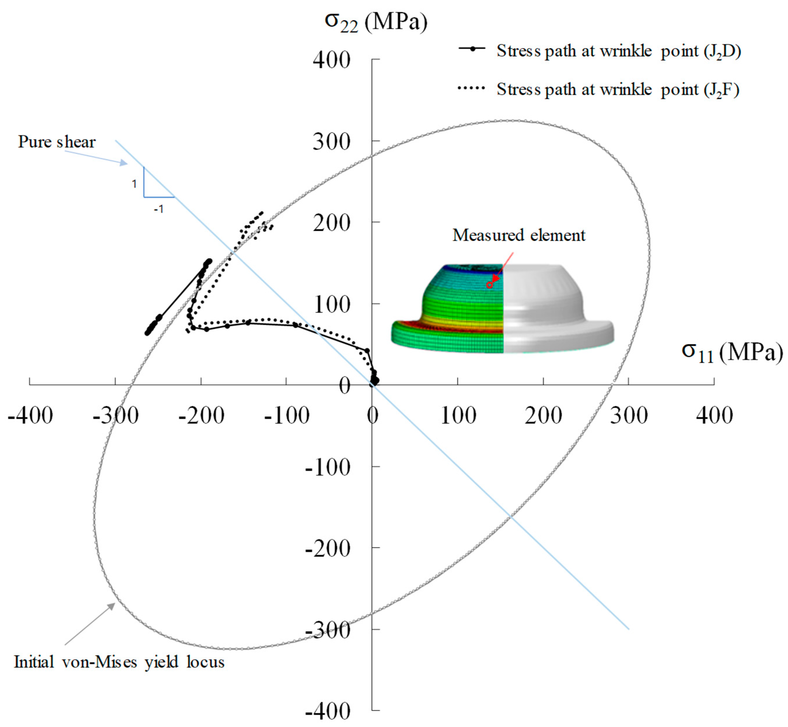
• The stress paths obtained using J₂F and J₂D were compared to confirm the difference between them and it was confirmed that the stress path obtained using J₂D was in the region dominated by compression.
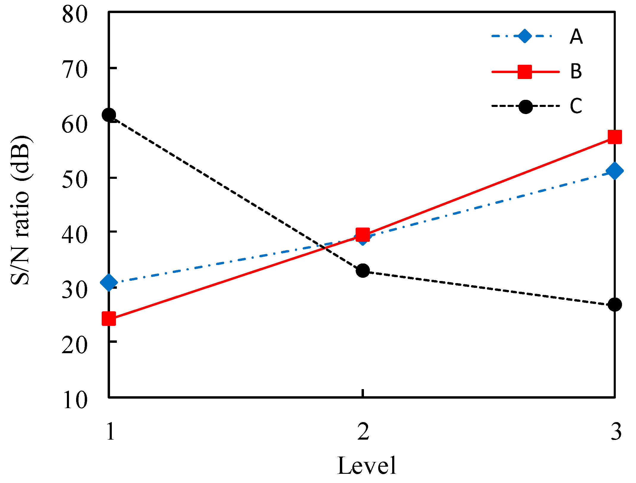
• To optimize the design parameters, the Taguchi method and ANOVA and ANOM analyses were employed along with FE simulations based on J₂D.
• The optimal condition for minimizing wrinkle formation was A₃B₃C₁, which means that the S/N ratio of the friction coefficient μ was optimized in level 3 (μ = 0.07), the blank thickness was optimized in level 3 (t = 0.28), and the outer profile angle was optimized in level 1 (α = 34), respectively.
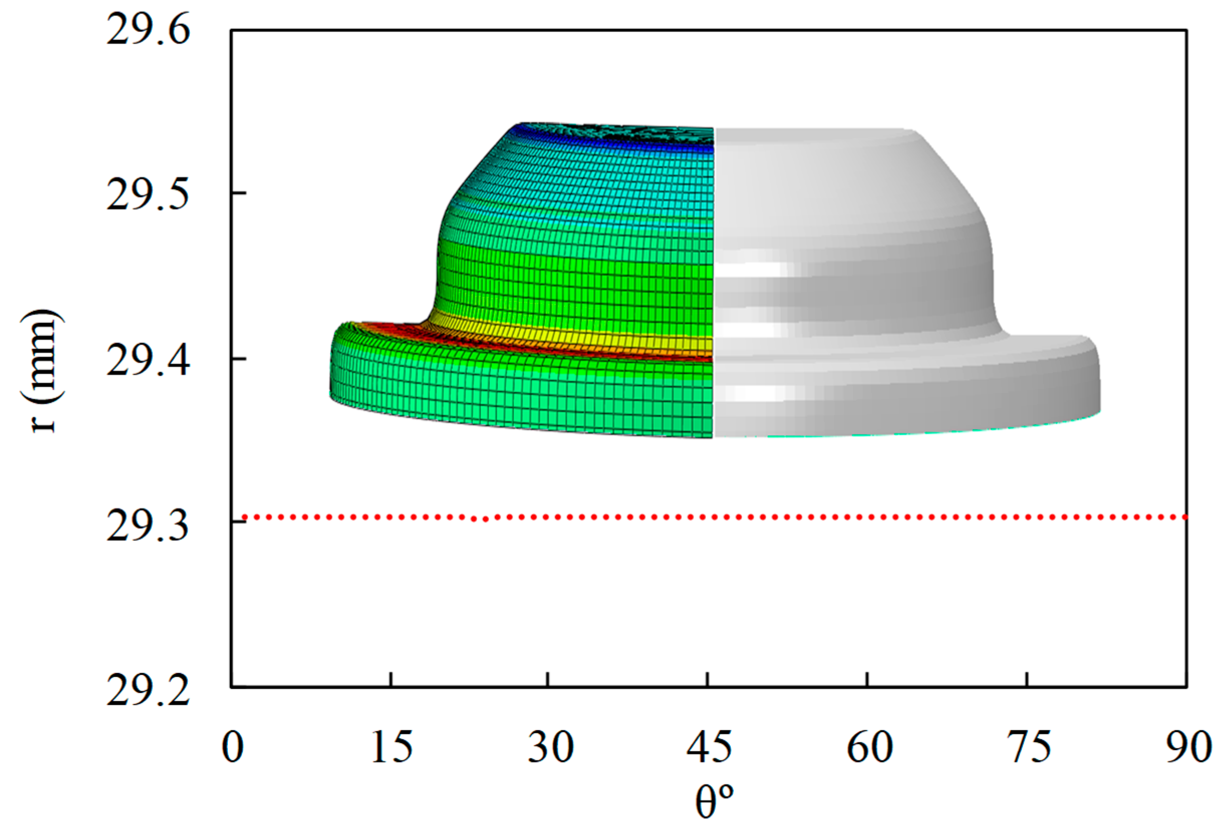
• A simulation with the optimal condition shows the result without wrinkle.

Based on the above results, the validity of the J₂D theory was demonstrated. When predicting many small-amplitude wrinkles, selection of the plastic strain calculation theory is more important than selection of the yield function. In addition, the optimization was performed by combining FE simulation based on J₂D and the Taguchi method to indicate the feasibility of such optimization. The parameters were validated by a simulation using J₂D. Based on the above results, the deformation theory is suitable for accurately predicting the occurrence of wrinkles and utilizing to optimize the influence parameters.

References

1. Moshksar, M.M.; Zamanian, A. Optimization of the tool geometry in the deep drawing of aluminum. J. Mater. Process. Technol. 1997, 72, 363–370. [Google Scholar] [CrossRef]
2. Jensen, M.R.; Damborg, F.F.; Nielsen, K.B.; Danckert, J. Optimization of the draw-die design in conventional deep-drawing in order to minimise tool wear. J. Mater. Process. Technol. 1998, 83, 106–114. [Google Scholar] [CrossRef]
3. Beritsprecher, T.; Wartzack, S. Neural network based modeling and optimization of deep drawing – extrusion combined process. J. Intell. Manuf. 2014, 25, 77–84. [Google Scholar] [CrossRef]
4. Pham, Q.T.; Kim, Y.S. Identification of the plastic deformation characteristics of AL5052-O sheet based on the non-associated flow rule. Met. Mater. Int. 2017, 23, 254–263. [Google Scholar] [CrossRef]
5. Pham, Q.T.; Lee, M.G. Characterization of the isotropic-distortional hardening model and its application to commercially pure titanium sheets. Int. J. Mech. Sci. 2019, 160, 90–102. [Google Scholar] [CrossRef]
6. Lee, H.S.; Jung, D.W.; Jeong, J.H.; Im, S.Y. Finite element analysis of lateral buckling for beam structures. Computers&Structures 1994, 53, 1357–1371. [Google Scholar] [CrossRef]
7. Riks, E. An incremental approach to the solution of snapping and buckling problems. Int. J. Solids Struct. 1978, 15, 529–551. [Google Scholar] [CrossRef]
8. Wang, X.; Lee, L.H.N. Postbifurcation behavior of wrinkles in square metal sheets under Yoshida Test. Int. J. Plast. 1993, 9, 1–19. [Google Scholar] [CrossRef]
9. Wang, C.T.; Kinzel, G.; Altan, T. Wrinkling criterion for an anisotropic shell with compound curvatures in sheet forming. Int. J. Mech. Sci. 1994, 94, 945–960. [Google Scholar] [CrossRef]
10. Tomita, Y.; Shindo, A. Onset and growth of wrinkles in thin square plates subjected to diagonal tension. Int. J. Mech. Sci. 1994, 36, 945–960. [Google Scholar] [CrossRef]
11. Gendy, A.S.; Saleeb, A.F. Generalized mixed finite element model for pre- and post-quasistatic buckling response of thin-walled framed structures. Int. J. Numer. Methods Eng. 1994, 37, 297–322. [Google Scholar] [CrossRef]
12. Cao, J.; Boyce, M.C. Optimization of Sheet Metal Forming Processes by Instability Analysis. In Proceedings of the 5th International Conference on Numiform, Itchaca, NY, USA, 18–21 June 1995; pp. 675–679. [Google Scholar]
13. Cao, J.; Boyce, M.C. Wrinkling behaviour of rectangular plates under lateral constraint. Int. J. Solids Struct. 1997, 34, 153–176. [Google Scholar] [CrossRef]
14. Cao, J.; Wang, X. An analytical model for plastic wrinkling under tri-axial loading and its application. Int. J. Mech. Sci. 2000, 42, 617–633. [Google Scholar] [CrossRef]
15. Wang, X.; Cao, J. On the prediction of side-wall wrinkling in sheet metal forming processes. Int. J. Mech. Sci. 2000, 42, 2369–2394. [Google Scholar] [CrossRef]
16. Makinouchi, A. Sheet metal forming simulation in industry. J. Mater. Process. Technol. 1996, 60, 19–26. [Google Scholar] [CrossRef]
17. Nam, J.B.; Han, K.S. Finite Element Analysis of Deep Drawing and Ironing Process in the Steel D&I Canmaking. ISIJ Int. 2000, 40, 1223–1229. [Google Scholar] [CrossRef]
18. Rekas, A.; Latos, T.; Budzyn, R.; Kociolek, M.; Styrna, T. Numerical simulations of drawing and redrawing process of forming thin cylindrical element from aluminium series 3XXXX. Key Eng. Mater. 2015, 641, 218–231. [Google Scholar] [CrossRef]
19. Kawka, M.; Olejnik, L.; Rosochowski, A.; Sunaga, H.; Makinouchi, A. Simulation of wrinkling in sheet metal forming. J. Mater. Process. Technol. 2001, 109, 283–289. [Google Scholar] [CrossRef]
20. Kim, Y.S.; Son, Y.J. Study on wrinkling limit diagram of anisotropic sheet metals. J. Mater. Process. Technol. 2000, 97, 88–94. [Google Scholar] [CrossRef]
21. Kim, J.B.; Yoon, J.W.; Yang, D.Y. Investigation into the wrinkling behaviour of thin sheets in the cylindrical cup deep drawing process using bifurcation theory. Int. J. Numer. Method Eng. 2003, 56, 1673–1705. [Google Scholar] [CrossRef]
22. Hutchinson, J.W.; Neale, K.W. Sheet necking-II. Time-independent behavior. In Mechanics of Sheet Metal Forming; Springer: Boston, MA, USA, 1978; pp. 127–153. [Google Scholar]
23. Hutchinson, J.W.; Neale, K.W. Finite Strain J2 Deformation Theory. In Proceedings of the IUTAM Symposium on Finite Elasticity, Bethlehem, PA, USA, 10–15 August 1980; Springer: Berlin/Heidelberg, Germany, 1982; pp. 237–247. [Google Scholar] [CrossRef]
24. Fleck, N.A.; Hutchinson, J.W. A phenomenological theory for strain gradient effects in plasticity. J. Mech. Phys. Solids 1993, 41, 1825–1857. [Google Scholar] [CrossRef]
25. Fleck, N.A.; Muller, G.M.; Ashby, M.F.; Hutchinson, J.W. Strain gradient plasticity: Theory and experiment. Acta Metall. Mater. 1994, 42, 475–487. [Google Scholar] [CrossRef]
26. Hutchinson, J.W. Generalizing J2 flow theory—Fundamental issues in strain gradient plasticity. Acta Mech. Sin. 2012, 28, 1078–1086. [Google Scholar] [CrossRef]
27. Cao, P.; Feng, D.; Zhou, C. A New Method to Achieve Equivalent Plastic Strain Explicit Form of J2 Plastic Isotropic Kinematic Hardening Model and Numerical Verification. Struct. Longev. 2012, 8, 193–206. [Google Scholar] [CrossRef]
28. Neal, K.W.; TuGcu, P. A numerical analysis of wrinkle formation tendencies in sheet metals. Int. Numer. Methods Eng. 1990, 30, 1595–1608. [Google Scholar] [CrossRef]
29. Dick, R.E.; Yoon, J.W. Wrinkling during Cup Drawing with NUMISHEET2014 Benchmark Test. Steel Res. Int. 2015, 86, 915–921. [Google Scholar] [CrossRef]
30. Barlat, F.; Brem, J.C.; Yoon, J.W.; Chung, K.; Dick, R.E.; Lege, D.J.; Pourboghrat, F.; Choi, S.H.; Chu, E. Plane stress yield function for aluminum alloy sheets-part 1: Theory. Int. J. Plast. 2003, 19, 1297–1319. [Google Scholar] [CrossRef]
31. Stören, S.; Rice, J.R. Localized necking in thin sheets. J. Mech. Phys. Solids 1975, 23, 421–441. [Google Scholar] [CrossRef] [Green Version]
32. Dick, R.E. Improvements to the Beverage can Redraw Process using LSDYNA. In Proceedings of the International LS DYNA Users Conference, Dearborn, MI, USA, 19–21 May 2002. [Google Scholar]
33. Ramberg, W.; Osgood, W.R. Description of Stress-Strain Curves by Three Parameters; National Advisory Committee for Aeronautics: Washington, DC, USA, 1943. [Google Scholar]
Figure 1. Configuration of process to fabricate beverage cans.
Metals 09 01168 g001
Figure 2. Occurrence of wrinkling on the bottom of a can.
Metals 09 01168 g002
Figure 3. True stress–true strain curves of the AA3104 sheet for three different orientations.
Metals 09 01168 g003
Figure 4. (a) Schematic diagram of the redraw process and (b) geometry for FE simulation with blank meshed.
Metals 09 01168 g004
Figure 5. Curve fitting result for Ramberg–Osgood model with experiment in the rolling direction.
Metals 09 01168 g005
Figure 6. FE simulation results: wrinkling prediction based on (a) J2F, (b) J2D, (c) wrinkle amplitudes along circumferential direction in experiment, and (d) schematic view of wrinkling measurements.
Metals 09 01168 g006
Figure 7. Evolution of the stress path of J2D and J2F in a wrinkle element with initial von Mises yield locus.
Metals 09 01168 g007
Figure 8. Cylindrical stress distributions along the (a) circular direction, σ θ (S22) and (b) radial direction, σ r (S11) according to punch stroke in the J2F-based simulation.
Metals 09 01168 g008
Figure 9. Cylindrical stress distributions along the (a) circular direction, σ θ (S22) and (b) radial direction, σ r (S11) according to the punch stroke in the J2D-based simulation.
Metals 09 01168 g009
Figure 10. Wrinkling mechanism: (a) view of no contact during redrawing and (b) stress mode of the element in which wrinkles occurred.
Metals 09 01168 g010
Figure 11. Effective strain of an element in the wrinkled area.
Metals 09 01168 g011
Figure 12. Signal-to-noise (S/N) ratio showing the wrinkle factor level from ANOM analysis.
Metals 09 01168 g012
Figure 13. Simulation result and wrinkle amplitudes along the circumferential direction.
Metals 09 01168 g013