Article

Using the Multi-Response Method with Desirability Functions to Optimize the Zinc Electroplating of Steel Screws

by
Ruben Lostado Lorza
1,*,
María Ángeles Martínez Calvo
1,
Carlos Berlanga Labari
2 and
Pedro J. Rivero Fuente
2
1
Department of Mechanical Engineering, University of La Rioja, 26004 Logroño, La Rioja, Spain
2
Institute for Advanced Materials (INAMAT), Department of Mechanical Engineering, Public University of Navarre—UPNA, Campus Arrosadía S/N, 31006 Pamplona, Navarre, Spain
*
Author to whom correspondence should be addressed.
Metals 2018, 8(9), 711; https://doi.org/10.3390/met8090711
Submission received: 24 August 2018 / Revised: 3 September 2018 / Accepted: 5 September 2018 / Published: 11 September 2018

Abstract

:
Zinc electroplating is a coating process controlled by several input process parameters. However, the commonly used input parameters for setting the process of zinc deposition are current density, temperature of the coating solution, zinc concentration, deposition time, and concentration of additives (conditioner and brightener). The power consumed in the zinc plating process, coating thickness, increase in coating mass, and corrosion resistance are considered to be outputs or zinc coating parameters. They are widely used when the zinc coating requirements are based on the coating process cost, coating process speed, corrosion resistance, and coating thickness. This paper seeks to determine regression models by the response surface method (RSM) that relate the zinc coating parameters to the input parameters in steel screws. When considering the coating requirements of cost, coating process speed, corrosion resistance, and coating thickness, the optimal input parameters were found by using a multi-response surface (MRS). Input parameters of 0.3 amps/dm2, 20.0 °C, 13.9 g/L, 45 min, 28.5 mL/L, and 2.8 mL/L, respectively (relative to the commonly used input parameters detailed above), were obtained when considering the cost. Considering minimization of the deposition time, the input parameters obtained were 0.5 amps/dm2, 24.6 °C, 13.9 g/L, 45 min, 26.9 mL/L, and 1.1 mL/L, respectively. The optimal inputs to maximize the corrosion resistance were 0.6 amps/dm2, 32.4 °C, 14.0 g/L, 45 min, 28.7 mL/L, and 2.5 mL/L, respectively. Finally, when maximizing the coating thickness, the inputs were 0.7 amps/dm2, 38.4 °C, 12.2 g/L, 45 min, 26.5 mL/L, and 1.5 mL/L, respectively.

1. Introduction

Zinc electroplating is one of the most commonly used methods to protect steel from the corrosion process. The reason for this is that it is a low-cost fabrication process in comparison to other deposition technologies. Thus, it is the preferred choice for many companies that keep a close eye on expenditures. The main way of using zinc to protect steel from corrosion is by sacrificial protection of the steel. This means that the zinc coating will be first to be corroded, instead of the metallic substrate, in order to increase the latter’s corrosion resistance [1,2,3]. One of the most important industrial applications of zinc electroplating is found in the automotive sector where it provides corrosion protection to brake pipes, brake calipers, and power steering components. It also can be employed in the military sector (tanks and armored personnel carriers) or as a protective coating prior to painting for better adhesion of paint to steel surfaces [4,5]. However, considerable efforts are continuously given to the development and implementation of new surface finishing processes for zinc plating due to the unending requirements of industry (especially in the automotive sector) for longer service life and better corrosion resistance in harsher environments [6,7,8]. Several strategies have been used to improve the corrosion resistance of zinc electroplating, such as using zinc alloy coatings [9,10]. As an example, Short et al. [9] demonstrated that the use of zinc-nickel electrodeposits that contain about 12–13% Ni promoted an increase in corrosion resistance compared with pure zinc electrodeposits. However, the effect of different factors, such as temperature, current density, time, zinc concentration, and additive concentration, on the corrosion rate has not been proven yet.
This process involves the electrolytic deposition of a thin coating of zinc onto the surface of the metal to be protected, which is known as a substrate. This process is governed by several factors. However, current density (ρ), temperature (T), and concentration of the zinc deposit (C) have the most significant influence on zinc deposition [11]. The current density (ρ) has a significant impact on the thickness of the zinc coating (Th). As a general rule, the thickness of the zinc coating obtained rises as the current density increases [12]. However, if the current density (ρ) exceeds a threshold value, a rough surface of the zinc substrate is generated, leading it to have a lower corrosion resistance (R) than if the surface was smooth [13]. At a higher temperature (T), there is an increase in the diffusion of hydrogen at the cathode. In addition, the absorption of hydrogen in metals is a serious problem during zinc electroplating. In fact, it is often said that a zinc layer acts as a barrier against hydrogen absorption. This greatly improves the mechanical and anticorrosive characteristics of the zinc coating. In addition, when the temperature (T) and the current density (ρ) increase at the same time, the deposited zinc is much brighter. On the other hand, when the temperature (T) increases and the current density (ρ) remains constant, the zinc coating is irregular, because the zinc crystals that are deposited on the substrate are very large [14]. Also, the concentration of zinc (C) in the coating solution affects the brightness and surface finish of the zinc deposit. Higher concentrations (C) will produce a rougher surface with large zinc crystals, whereas lower concentrations will provide a brighter finish with finer and more corrosion-resistant crystals [15]. In recent decades, some scientific studies have been conducted to determine which factors are most important in improving the performance of the zinc plating process [16,17].
However, these scientific studies have not been supported by multivariate statistical techniques that investigate how one factor influences the other factors. One of the most frequently used techniques used to study the influence of a factor or input on the others and then optimize the combination of factors to obtain the best output is response surface methodology (RSM) [18,19]. When there is more than one output, several response surfaces should be optimized using the multi-response surface method (MRS) [20]. In this paper, a group of regression models that are based on the RSM were used to relate the zinc coating requirements (outputs) to the zinc coating process parameters (inputs). The latter were current density (ρ), temperature of the coating solution (T), zinc concentration (C), deposition time (t), concentration of Additive 1 (Envirozin Conditioner (CA1)), and concentration of Additive 2 (Envirozin 100 Initial Brightener (CA2)). The response surface method (RSM) for steel screws was used. Then, while considering zinc coating requirements based on cost, manufacturing speed, corrosion resistance, and coating thickness, the optimal input process parameters were found by using the multi-response surface (MRS) with the desirability functions. The power consumed in the zinc plating process (W) and the increase in coating mass (ΔM) are the zinc coating process parameters that are used when the zinc coating requirements are based on cost. However, the deposition time (t) is the parameter that is used when the zinc coating process parameters requirements are based on the electroplating process speed. Corrosion resistance (R) is the parameter used when the zinc coating process parameter requirements are based on the corrosion resistance. Finally, zinc coating (Th) is the parameter used when the zinc coating process parameters requirements are based on the coating thickness. This paper concentrates on a study of the zinc electroplating process in steel screws for the following ranges: current densities (ρ), 2–3 amps/dm2; temperature (T), 30–40 °C; concentration of zinc deposit (C), 8–14 (g/L); time (t), 30–60 min.; Concentration Additive 1 (CA1), 8–10 (mL/L); and Concentration Additive 2 (CA2), 1–3 (mL/L). Figure 1 shows a scheme in which all inputs and outputs that were considered in this work are used for modeling and optimizing the zinc electroplating process of screws.

2. Modeling and Optimizing Using the RSM with Desirability Functions

The RSM seeks to determine the relationships of input variables (independent variables) to output variables (response variables). It was developed as a means to model experimental responses. Box and Wilson introduced the method in 1951 [18] to create a model for optimal response with the data provided by experiments. It has been used recently along with other techniques for the optimization of products and industrial processes [21,22,23,24]. In essence, the RSM is a collection of statistical techniques that uses a regression model based on a low-degree polynomial function (Equation (1)):
Y = f ( X 1 , X 2 , X 3 , , X k ) + e  
where Y is an experimental response, (X1, X2, X3, …, Xk) is the input vector, e is an error term, and f is a function of cross-products of the polynomial’s terms. The quadratic model (second-order) is a widely-used polynomial function. It appears in Equation (2):
Y = b 0 + i = 1 n b i X i + i = 1 n b ii X i 2 + i = 1 n 1 j = i + 1 n b ij X i X j + e  
where the linear part is the first summation, the quadratic part is the second, and the product of the pairs of variables is the third. The coefficients b0, bi, bii, and bij are determined using regression analysis. However, satisfactory results are not always obtained from these functions for complex problems that have many inputs and nonlinearities. The reason for this is that continuous functions are defined by polynomials. Thus, if data are insufficient, the functions cannot be adjusted. The p-value (or Prob. > F) is the probability of receiving a result that equals or exceeds what was observed. This assumes that the model is accurate. It can be determined by analysis of variance (ANOVA). If the Prob. is greater than the F value of the model and the model has no term with a level of significance that exceeds, for example, α = 0.05, the model will be acceptable at a confidence interval of (1 − α). Some researchers have employed ANOVA to determine the inputs’ or process parameters’ influence on the zinc plating process outputs [25,26]. If there is more than one output, the problem is termed an MRS. This implies that the outputs are in disagreement. There can be a great difference between the optimal configurations for different outputs. Harrington [27] proposed a compromise between outputs, comprising desirability functions for each output, as shown in Equations (3) and (4), and an overall desirability measure, namely, the geometric mean D of each output’s desirability (Equation (5)).
d r max = { 0 if   f r ( X ) < A ( f r ( X ) A B A ) S if   A f r ( X ) B 1 if   f r ( X ) > B  
d r min = { 1 if   f r ( X ) < A ( f r ( X ) B A B ) S if   A f r ( X ) B 0 if   f r ( X ) > B  
D = ( r = 1 R d r ) 1 / R  
In the equations above, A and B are limit values and the exponent s determines the importance of achieving the target value; X is the input vector and fr is the model used in the prediction. To optimize one or more responses, one should use a higher-degree polynomial [28]. The desirability approach requires that each estimated response be transformed into a unitless utility whose boundaries are 0 < dr < 1, where higher values of dr indicate more desirable response values. The optimization portion of the R package v.1.6 looks for a combination of factors (or weights in the range 1–3) that simultaneously satisfy the optimization criteria of all responses and inputs.

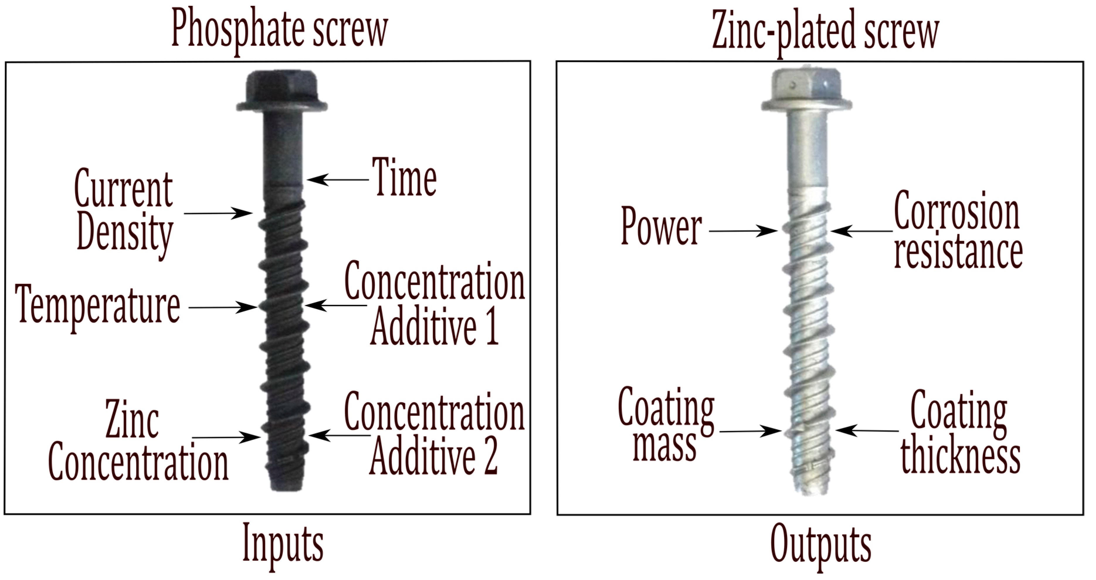
3. Electroplating Process Factors Examined by Use of RSM

Researchers have previously employed RSM to identify an optimal combination of process parameters or inputs for the electroplating process. However, most of their works have been based on modelling and optimizing the electroplating process and have involved relatively few input and output parameters. For example, Oraon et al. [29] used multi-response optimization of the nickel electroplating process to model the deposited mass per unit area (g/cm2) considering the concentration of NiCl2·6H2O, the concentration of NaBH4, and the temperature (°C) as the nickel coating process input parameters. In this case, they observed that reducing the concentration of NiCl2·6H2O, the concentration of NaBH4, and the temperature significantly influenced the deposition of the nickel coating. Santana et al. [30] studied the optimization of the electrolytic bath for electro-deposition of corrosion-resistant Fe–W–B alloys using multi-response optimization. In their case, a full factorial design was considered for the design of the experiments. Other authors, such as Poroch et al. [31], used multi-response optimization combined with a genetic algorithm to optimize the nickel electroplating process in order to improve the cathode efficiency, coating thickness, brightness, and hardness of the metallic layer. They used the nickel coating process input parameters of current density (amps/dm2), temperature T (°C), and pH. More recently, Poroch et al. [32] studied the modelling and optimization of nickel-iron electroplating process variables to maximize the surface hardness while considering current density (amps/dm2), temperature (°C), and pH as input factors. Also, Poroch et al. [33] used the design of experiments and response surface methodology to model and optimize an Fe-Ni electroplating process from a chloride-sulphate bath. They optimized the Fe-Ni electroplating process by using the desirability function approach.

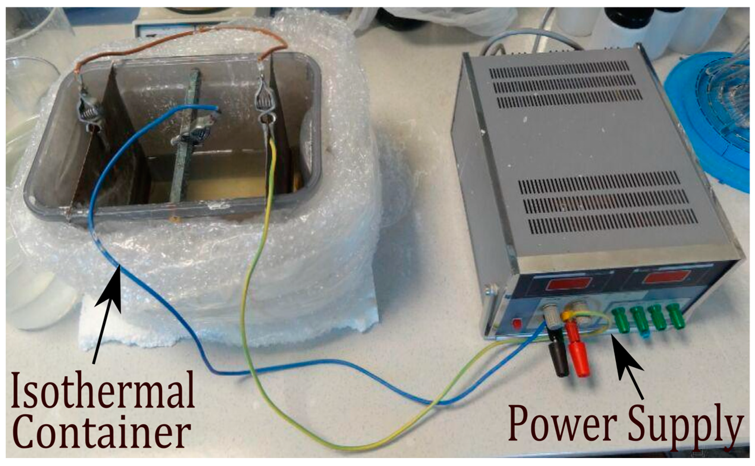
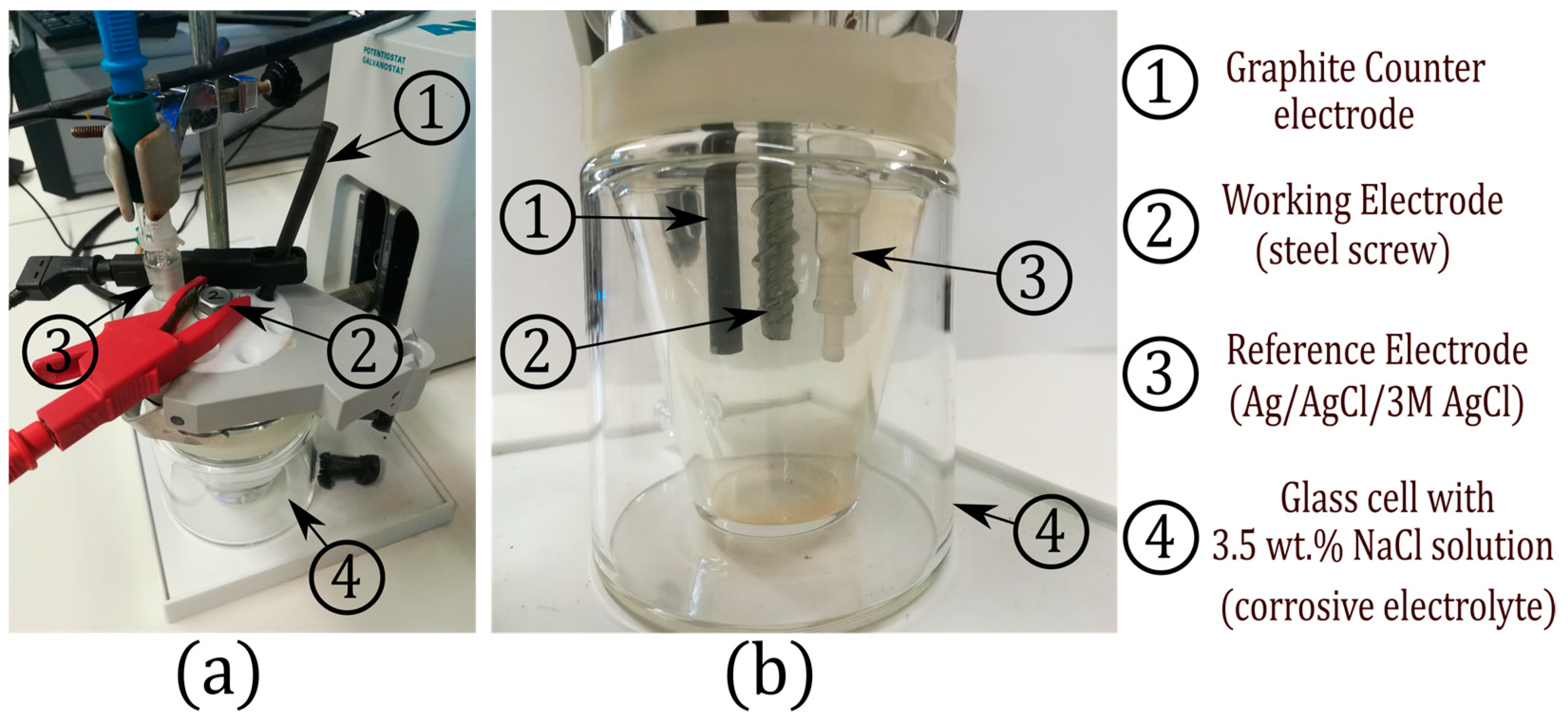
4. Experimental Setup and Results

Before undertaking the zinc electroplating process, all steel screws were subjected to a standard zinc phosphating process. This was done to provide a foundation for improvement of the adhesion of the coating to be applied to steel parts. Then, each of the phosphate screws was weighed on a precision balance to determine its initial mass prior to application of the zinc coating. The zinc electroplating process was then carried out in an isothermal container that was connected to an adjustable heater, into which each proposed solution was poured. These solutions were proposed based on zinc concentration (C), sodium hydroxide concentration, additive concentration 1 (CA1; Envirozin Conditioner), and additive concentration 2 (CA2, Envirozin 100 Initial Brightener). The positive pole of the power supply was connected to a pure zinc plate that served as a cathode. The negative pole was connected to the already phosphated steel screws, which served as the anode. Once the temperature of the previously proposed solution had been reached, each of the screws was completely immersed in this specific solution. Next, the power supply was connected and the values of intensity and voltage for the deposition of the proposed zinc coatings were adjusted until the values of the proposed current densities (ρ) were reached. The current density values were obtained from the current provided by the power source and from the surface of the screw. The current was measured using the power supply’s ammeter, whereas the surface of the screws was obtained theoretically using Catia v5 R18 (Woodlands Hills, CA, USA) [34]. However, for the purpose of always keeping the exposed surface of the screws unchanged, the position of the screws inside the isothermal container was also left unchanged, as well as the distance between the cathode and the anode. Figure 2 shows the proposed installation of the zinc electroplating of the phosphate screws.
After the time (t) for the deposition of the coating had elapsed, the power supply was disconnected, and the zinc-plated screw was withdrawn from the solution and then submerged in pure water to remove the dissolution residues from its surface. Then, the zinc-plated screw was immersed for 30 s in a passivating product (TRIPASS ECO 3) and subsequently immersed for 60 s in a sealant product (Hydroklad 30). After the zinc-plated screws that had been treated with the passivant and sealant were completely dry, they were weighed again on the precision scale. The difference in masses between the phosphate and galvanized screws was the coating mass increase (ΔM). The coating thickness measurement (Th) was conducted by means of a nondestructive technique that is based on the magnetic induction phenomenon and is in accordance with ASTM B499-09 [35]. A measuring device Minitest (Model 1100, Elektrophysik, Cologne, Germany) that was equipped with an FN 1.6-type probe was selected in this case for use when dealing with zinc coatings on steel substrates. The measurement of the coatings was made at four different points on each of the galvanized screws and an average value of the coatings was subsequently calculated. In order to validate and adjust this method of measuring the thickness, the thickness of the coatings of several of the zinc-plated steel screws was measured by means of destructive tests based on metallographic methods according to the ASTM E3-95 standard [36]. The corrosion resistance of all samples obtained by the zinc electroplating process was evaluated by taking electrochemical measurements using a potentiodynamic polarization technique [37]. Open-circuit potential (OCP) measurement and linear potential scan experiments were chosen as the electrochemical measurement methods. The measurements were conducted using an AUTOLAB-PGSTAT computer-controlled potentiostat (Metrohm, Herisau, Switzerland) in a naturally aerated 3.5 wt. % NaCl solution at room temperature. For this purpose, a conventional three-electrode cell was used with a graphite bar as counter electrode, an Ag/AgCl/3 M KCl electrode as reference electrode, and the specimen (steel screw) as a working electrode [38,39,40,41,42]. A glass cell containing 150 mL of 3.5 wt. % NaCl solution (corrosive electrolyte) was used for each electrochemical experiment. Figure 3a shows the connections made to each of the electrodes while Figure 3b shows the placement of each of the electrodes inside the glass cell.
The open-circuit potential for each sample was measured until a steady-state value was reached. Then, a linear potential sweep in the anodic direction was conducted at a scan rate of 1 mV/s, but beginning at 0.1 V below OCP and terminating at 0.1 V above the OCP. The output from these experiments yielded a polarization curve of the current density versus the applied potential. The resulting corrosion current can be calculated by using Tafel slope analysis where the relationship between the current density and the electrode potential during the polarization is obtained by the following equation (Equation (6)):
  I   = I c o r r   [ e 2.303 ŋ b a e 2.303 ŋ b c ]  
  ŋ   = E E c o r r  
where E is the electrode potential, I is the measured current density, ŋ is the difference between the applied electrode potential and the corrosion potential, Ecorr is the corrosion potential of the corroding metal, Icorr is the corrosion current, and ba, bc are the Tafel constants of anodic and cathodic half-cell reactions, respectively. Values for Tafel plots are derived from the logarithm of current density values as a function of voltage. More details of the fitting method for obtaining the corrosion parameters can be found elsewhere [43]. The corrosion data that were obtained from Tafel polarization curves were obtained by superimposing a straight line on the linear portions of the cathodic and anodic curves. It is important to note that the Tafel polarization curve is the most efficient method for detecting the anticorrosion performance of metal surfaces. In this sense, an excellent corrosion resistance is associated with a lower corrosion rate, which corresponds to a higher corrosion potential (Ecorr) or a lower corrosion current density (Icorr), respectively [44,45]. Finally, other corrosion parameters, such as equivalent weight of the metal, density, or exposed surface, are required as input parameters. With this information, the AUTOLAB software (Model 30, PalmSens, Houten, The Netherlands) generates the complete set of corrosion parameters. Thus, the corrosion rate is calculated according to Equation (8):
  C o r r o s i o n   r a t e = 327   ×   I c o r r   × M V   ×   D   ×   A  
where 327 = 1 year (in seconds)/96,500, and 96,500 = 1 F in coulombs. Icorr is the corrosion current and is determined by an intersection of the linear portions of the anodic and cathodic sections of the Tafel curves, M is the atomic mass, V is the valence (number of electrons that are lost during the oxidation reaction), D is the density, and A is the exposed area of the sample [44].

5. Design of Experiments

To provide accurate models without a great deal of data to support the original hypotheses, the RSM must establish a Design of Experiments (DoE) [46]. There are several methods to develop a DoE. However, they require that a design matrix (inputs) be constructed for the measurement of the outputs or experiment responses. In this case, we used a Box-Behnken design (BBD) [47] that had three factors, as well as three levels, to develop the experiment. The input process parameters that were used to develop the DoE were current density (ρ), temperature (T), time (t), concentration of zinc (C), concentration of Additive 1 (Envirozin Conditioner (CA1)), and concentration of Additive 2 (Envirozin 100 Initial Brightener (CA2)). The outputs were the power consumed in the zinc plating process (W), coating thickness (Th), the increase in the coating mass (ΔM), and corrosion resistance (R). The range of study considered in this case for each of the input process parameters was based on a preliminary group of phosphate screws to which a zinc coating was applied. The coating was applied to ensure that the galvanized screws had no defects or imperfections. Coatings were rejected if they presented a very irregular and/or rough coating, a reduced coating thickness (Th), a high temperature (T), or even an excessive deposition time (t). For example, Figure 4 shows some of the metallographic analyses that were obtained from the preliminary zinc coating and examined with a 50× microscope. Figure 4a shows a zinc coating with a thickness of 20 to 25 μm. The coating was formed with irregular zinc crystals, which create a very rough surface finish. In this case, and according to [11], the current density value considered was high (1.3 amps/dm2), whereas the considered solution temperature was low (20 °C). Figure 4b shows a coating that has a thickness of 25 to 30 μm. In this case, the temperature was excessive (48 °C), whereas the current density value considered was 0.5 amps/dm2. In this case, and according to [14], the coating surface was very rough and contained large zinc crystals. Figure 4c shows a homogeneous coating that was formed by small crystals and had a thickness of 7 to 8 μm. In this case, the values of current density, temperature, and deposition time were 0.32 amps/dm2, 30 °C, and 20 min, respectively. The crystals that formed had a reduced size. According to [15], the coating provides a brighter finish with finer crystals and is more corrosion resistant. In contrast, the coating had a reduced thickness, which was due mainly to the deposition time, which was reduced. Finally, Figure 4d shows a homogeneous coating that was formed by small crystals and a thickness of 24 to 25 μm. The values of current density, temperature, and deposition time considered in this case were 0.3 amps/dm2, 25 °C, and 90 min, respectively. The homogeneous coating was formed by small crystals with a brighter finish and higher corrosion resistance [17]. The search process to fix the parameters that did not generate effects or imperfections on the galvanized screws was carried out successively. It included other parameters, such as concentration of zinc (C), concentration of Additive 1 (CA1), and concentration of Additive 2 (CA2). After these were discarded, the ranges of all input process parameters were set. The input process parameters and their limits, as well as the notation, all appear in Table 1.
Use of the statistical open source software R (r-project) [48] and the input parameters and levels that appear in Table 1 led to the manufacture of 54 zinc-electroplated steel screws with the corresponding inputs and outputs obtained experimentally (Table 2).

6. Results and Discussion

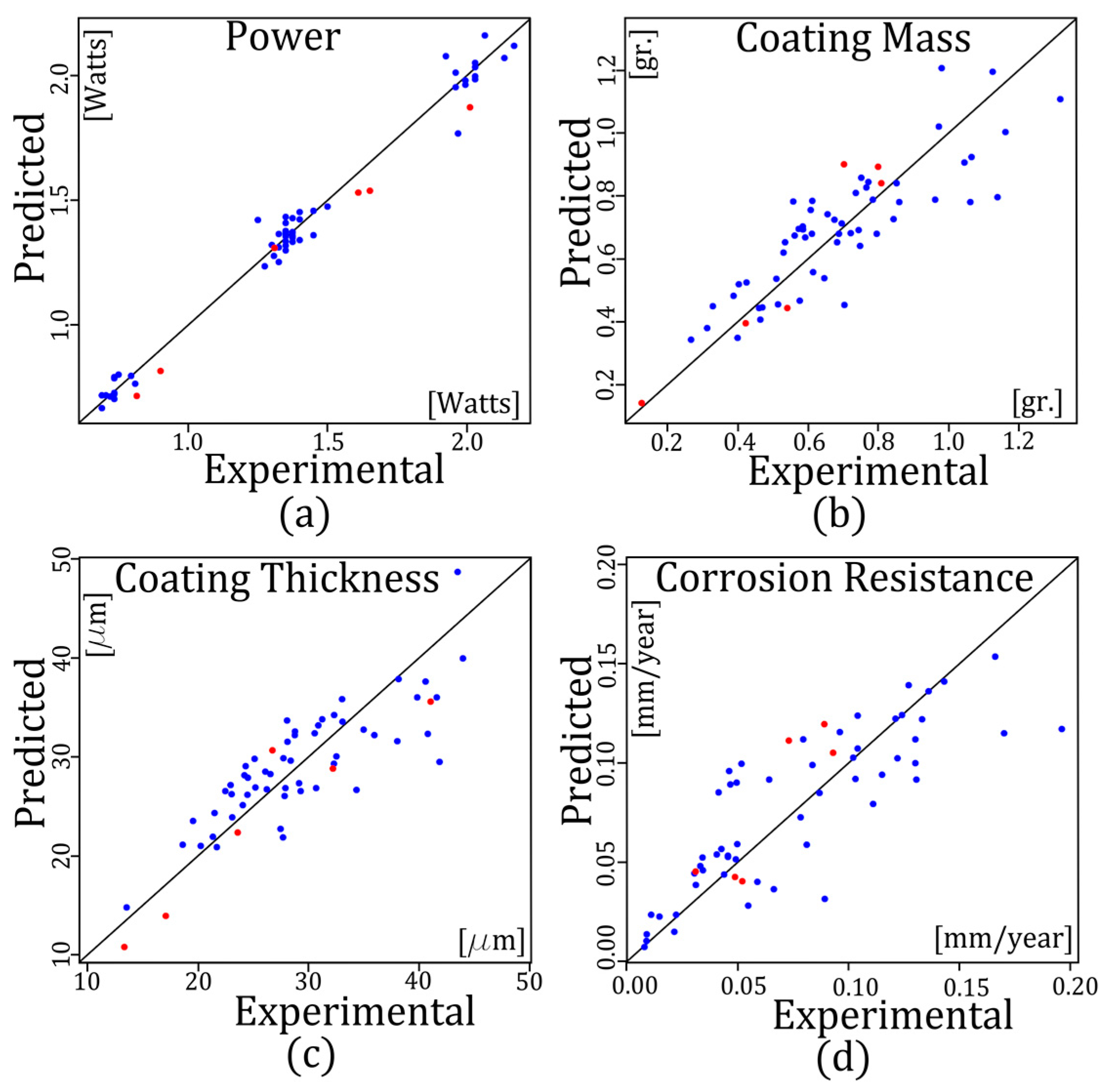
6.1. Modelling the W, Th, ΔM, and R Using RSM

The data in Table 2 were used to fit Equations (9)–(12) to provide regression equations for all responses. The RMS “R” package [28] was employed for this. Second-order polynomial models were constructed for each response. Selection of the most accurate model involved several criteria. These were R2, p-value, Mean Absolute Error (MAE), and Root Mean Squared Error (RMSE). The second-degree polynomial functions that modeled the power consumption of the zinc plating process (W), the increase in coating mass (ΔM), the zinc coating (Th), and the corrosion resistance (R) are shown in the equations. These equations show that each output is provided by a combination of second-order polynomials. The latter are formed, in turn, by combinations of input variables.
W = −5.626 + 3.660 × ρ + 0.129 × C − 0.087 × ρ × C+0.0015 × T × C − 0.0066 × C2 + 0.0031 × ρ × t + 0.0004 × C × t + 0.348 × CA1 − 0.00082 × T × CA1 − 0.00023 × t × CA1 − 0.0057 × CA12 − 0.323 × CA2 + 0.192 × ρ × CA2 + 0.0091 × CA1 × CA2
ΔM = 0.894 − 1.170 × ρ2 − 0.170 × ρ + 0.0027 × T × C + 0.029 × ρ × t − 0.00074 × T × t + 0.0016 × C × t − 0.00011 × t2 + 0.0023 × T × CA1 + 0.990 × CA2 − 0.0182 × T × CA2 − 0.049 × CA1 × CA2 + 0.185 × CA22
Th = −77.0078 − 79.377 × ρ2 + 9.251 × ρ + 0.190 × T × C − 0.702 × C2 − 0.0167 × T × t + 0.069 × C × t − 0.00293 × t2 + 4.754 × ρ × CA1 + 55.864 × CA2 − 20.573 × ρ × CA2 − 0.413 × T × CA2 − 0.858 × C × CA2 − 1.460 × CA1 × CA2 + 3.095 × CA22
R = −0.860 + 0.0419 × T − 0.00031 × T2 + 0.0687 × ρ × C + 0.00125 × C2 + 0.0078 × t − 0.00708 × ρ × t − 0.00085 × C × t − 1.835 × 10⁻⁵ × t2 − 0.0171 × ρ × CA1 − 0.000903 × T × CA1 + 0.00035 × t × CA1 + 0.00247 × T × CA2 − 0.0045 × C × CA2 − 0.00099 × t × CA2 + 0.0102 × CA1 × CA2 − 0.0638 × CA22
The results of ANOVA for all final quadratic models appear in Table 3, Table 4, Table 5 and Table 6. The p-value of most variables is less than 0.01. Thus, the inputs that the reduced quadratic models used are statistically significant. Similarly, it can be seen in these tables that ρ is the most influential input for “W” (Table 3), since the p-value is <2.2 × 10⁻¹⁶, whereas CA1 is the most influential input for “ΔM” (Table 4) and “Th” (Table 5), since it has p-values of 0.0025282 and 0.00005107, respectively. Additionally, the measure of the variation around the mean of the regression model’s results was used as the multiple correlation coefficient (R2). All values of R2 were close to 1. Thus, these models possess good predictive capacity.
Also, MAE and RMSE were calculated in order to identify the quadratic models’ generalization capacity, using the data in Table 2, according to Equations (13) and (14):
MAE = 1 m k = 1 m | Y k   Experiment Y k   Model |  
RMSE = 1 m k = 1 m ( Y k   Experiment Y k   Model ) 2  
where Yk Experiment are the experimental responses in this case, and Yk Model are the responses from the quadratic models that were obtained with the quadratic regression models and the specimens, m. The prediction errors MAE and RMSE that appear in Table 7 occurred when the maximum error corresponded to Th (an MAE of 10.48% and an RMSE of 12.73%). The minimum error corresponded to W (an MAE of 2.77% and an RMSE of 3.87%).
Additionally, six new zinc-coated steel screws were created. They were used for testing the proposed regression models with previously unused regression model parameters. These new six steel screws were generated randomly. Table 8 shows the inputs and outputs of these six new zinc-coated steel screws.
Once the new six new zinc-coated steel screws were manufactured, the errors that arose during the testing stage were calculated (See Table 9). This table shows that the maximum error corresponds to Th (an MAE of 10.81% and an RMSE of 11.58%), whereas the minimum error corresponds to W (an MAE of 5.9% and an RMSE of 5.57%). The errors indicate that the adjustment of the regression models and the results of the zinc-coated steel screws are relatively accurate. It also indicates a good generalization capacity.
After the errors in the prediction from the regression models of the training and testing data were made, a scatter diagram of the variables was created. Figure 5 shows the scatter diagram or relationship of the experimental values to the values that had been predicted (quadratic models) for W, ΔM, Th, and R. The blue points correspond to the 54 datapoints shown in Table 2, whereas the red points correspond to the six additional zinc-coated steel screws that were used in the regression models that appear in Table 8. In this case, if the variables are correlated, the points will fall along the diagonal line or curve. The better the correlation, the tighter the points will hug the line. The figures indicate that all the red dots (or test data) are closer to the diagonal line than are some of the blue dots (or training data). Therefore, their correlation is greater. Because the number of test datapoints is less than the number of training datapoints, the MAE and RMSE errors for the testing analysis and the training analysis are similar (see Table 8 and Table 9). However, the variables that had the greatest correlation were W and ΔM, whereas the variables that had the lowest correlation were Th and R. The reason for this may be that the procedure to obtain these variables is more complex than the one to obtain W and ΔM, and, therefore, the error may be greater. As a result of the figures and the errors shown in Table 8 and Table 9, it can be said that these models suffice for the prediction of such values, as the residuals were small and the correlations of actual to predicted values were high.

6.2. Multi-Response Optimization

Table 10, Table 11, Table 12, Table 13, Table 14, Table 15, Table 16 and Table 17 show the combinations of input parameters that were examined when looking for the optimal process for zinc electroplating of steel screws by means of the RMS “R” package and desirability functions while considering several optimization criteria or scenarios. The first column of Table 10, Table 11, Table 12, Table 13, Table 14, Table 15, Table 16 and Table 17 provides the input and output zinc coating process parameter requirements that were studied. The second column indicates the optimization process objective for inputs and outputs. The third and the fourth columns in the tables show the minimum and maximum values that can be reached for process parameters and characteristics of the zinc coating (range) according to Table 1. Finally, the fifth column shows the values of the electroplating process parameters and characteristics of the zinc coating that are achieved, whereas the sixth column shows the obtained desirability values. The results of the optimal zinc electroplating process based on the coating process cost are shown in Table 10. In this case, the coating process cost was based on minimizing the power consumed (W), minimizing the temperature (T), and minimizing the coating mass (ΔM). The value of the overall desirability was 0.98 in this case. Table 11 shows the results for the zinc electroplating process based on the coating process speed which, in turn, is based on the minimization of deposition time (t). In this case, the value of the overall desirability was 1. Table 12 shows the results for the optimal zinc electroplating process based on maximizing the corrosion resistance of the coating (R). The value of the goal that was established was the maximum, and the overall desirability was 1. Table 13 shows the results for the optimal zinc electroplating process based on maximizing the coating thickness (Th). The overall desirability in this case was 1. Table 14 shows the results for the optimal zinc electroplating process based on maximizing the resistance (R) while minimizing the temperature (T), the concentration (C), and the deposition time (t). The overall desirability in this case was 0.73. Table 15 shows the results for the optimal zinc electroplating process based on maximizing the thickness (Th) while the temperature (T), the concentration (C), and the time (t) are minimized. In this case, the value of the overall desirability was 0.79. Finally, Table 16 shows the results for the optimal zinc electroplating process based on maximizing the thickness (Th) and the resistance (R), while the temperature (T) and the concentration (C) are minimized. The overall desirability obtained in this last case was 0.74. The results that appear in Table 10, Table 11, Table 12, Table 13, Table 14, Table 15 and Table 16 show that the process parameters differ greatly for the various optimal zinc electroplating processes that were studied.
After obtaining the proposed optimal zinc electroplating process, seven new zinc-coated steel screws were manufactured in order to test the proposed methodology’s accuracy. The manufacturing of the zinc-coated steel screws followed the combination of process parameters that appears in Table 10, Table 11, Table 12, Table 13, Table 14, Table 15 and Table 16 and under conditions identical to those described in Section 4. The values of the outputs or zinc coating parameters of these eight new screws are shown in Table 17. In order to examine the different errors in predicting outputs or zinc coating parameters by the eight optimal zinc coating criteria, MAE and RMSE were developed with data that had been normalized. Data is frequently normalized in statistical processes to convert all variables to a common scale (from 0 to 1). This transformation was effected in this case by deducting from each original value the minimum value, and then dividing by the range of each variable as per Equation (15):
Y k ,   n o r m = Y k min ( Y ) r a n g e ( Y )  
where Yk, norm are the normalized outputs from outputs or zinc coating parameters from models developed with RSM and the zinc coating parameters or experimental outputs. The error in the last two columns of Table 17 represents the MAE and RMSE which were normalized for all variables of the eight criteria that were studied. The normalized MAE and RMSE in the last two rows of the table relate to the errors in the zinc coating parameters or outputs that were studied. For example, when the first criterion is considered (minimizing the power consumed), the errors obtained are smallest (MAE = 4.9% and RMSE = 7.3%). However, when the fifth criterion is considered (maximizing the resistance (R) and minimizing the temperature (T), the concentration (C), and the time (t)), the error is greatest (MAE = 7.7% and RMSE = 9.8%). The reason for this difference in the errors could be that both the experimental measurement and the regression model to obtain the power consumed in the zinc electroplating process (W) are very precise (see Table 7 and Table 9), so the total MAE and RMSE may be the lowest. However, the experimental measurement and the regression models that were used to obtain the thickness (Th) and corrosion resistance (R) at the same time are not very precise (see Table 7 and Table 9). Thus, the total MAE and RMSE may be the highest. Similarly, the maximum errors for the zinc coating parameters or outputs are lower when predicting the power consumption (MAE = 2.7% and RMSE = 2.9%) and greater when predicting thickness (MAE = 12.5% and RMSE = 13.4%). The MAE and RMSE values for all zinc-electroplated steel screw parameters or outputs are in acceptable agreement.

7. Conclusions

This paper presents a methodology that permits the optimization of a zinc electroplating coating process in steel screws when several optimization scenarios are considered simultaneously. First, a DoE using BBD determined the configuration for electroplating 54 zinc steel screws. Using RSM, the power consumed in the zinc plating process, coating thickness, increase in coating mass, and corrosion resistance were modeled by quadratic regression models as functions of the input parameters. The latter were current density, temperature of the coating solution, zinc concentration deposition time, and concentration of additives (conditioner and brightener). The resulting models were tested and deemed to be acceptable. A multi-objective optimization study that used the desirability function approach was conducted. It considered several optimization criteria or scenarios. These included manufacturing cost, manufacturing speed, corrosion resistance, and coating thickness of the zinc plating process. In the optimization study results, the point at which the current reached its optimum value ranged from 0.3 amps/dm2 to 0.7 amps/dm2 for current density, 20 °C to 38.371 °C for temperature, 9.555 g/L to 14.0 g/L for concentration of zinc, 45.0 min to 89.717 min for time, 25.021 mL/L to 29.967 mL/L for conditioner (Additive 1), and 1.099 mL/L to 2.814 mL/L for brightener (Additive 2). The results suggest that optimal process parameters are found when various design requirements are satisfied in a range that is relatively small. This is particularly the case for time, given that most process instances were 45 min in length. Finally, seven zinc-electroplated steel screws with optimal zinc coating requirements were manufactured in order to test the proposed methodology’s accuracy. The experimental and predicted results were found to be in good agreement.

Author Contributions

Experimental work: R.L.L., M.Á.M.C., C.B.L. and P.J.R.F. Development of predictive models and optimization: R.L.L. and M.Á.M.C. Results analysis and manuscript preparation: all authors.

Funding

This research received no external funding.

Acknowledgments

The authors wish to thank the University of La Rioja for its support through Project ADER 2014-I-IDD-00162.

Conflicts of Interest

The authors declare no conflict of interest.

References

  1. Yli-Pentti, A. Electroplating and electroless plating. In Comprehensive Materials Processing; Elsevier: Oxford, UK, 2014; pp. 277–306. [Google Scholar]
  2. Pourbaix, M. Applications of Electrochemistry in Corrosion Science and in Practice. Corros. Sci. 1974, 14, 25–82. [Google Scholar] [CrossRef]
  3. Schneider, S. Zinc Plating. Plat. Surf. Finish. 2007, 94, 40–41. [Google Scholar]
  4. Oluwole, O.O.; Oloruntoba, D.T.; Awheme, O. Effect of Zinc Plating of Low Carbon Steel on Corrosion Resistance in Cocoa Fluid Environment. Mater. Des. 2008, 29, 1266–1274. [Google Scholar] [CrossRef]
  5. Valentini, C.R.; Fiora, J.; Iglesias, A.M. Corrosion Behavior of Chromatized Zinc-Electroplated Mild Steel. Corrosion 2008, 64, 891–899. [Google Scholar] [CrossRef]
  6. Motte, C.; Maury, N.; Olivier, M.-G.; Petitjean, J.-P.; Willem, J.-F. Cerium Treatments for Temporary Protection of Electroplated Steel. Surf. Coat. Technol. 2005, 200, 2366–2375. [Google Scholar] [CrossRef]
  7. Yoshikawa, Y.; Imai, K.; Kimoto, M.; Hirose, Y.; Fukui, K.; Wakano, S. Performance of New Composite Zinc Electroplated Steel Sheet. SAE Tech. Pap. 1999. [Google Scholar] [CrossRef]
  8. Zhao, Y.P.; Yin, R.H.; Cao, W.M.; Yuan, A.B. Electropolymerization of Aniline on Zinc-Electroplated Steel from Neutral Aqueous Medium by Single-Step Process. Acta Met. Sin. 2004, 17, 849–855. [Google Scholar]
  9. Short, N.R.; Abibsi, A.; Dennis, J.K. Corrosion resistance of electroplated zinc alloy coatings. Trans. Inst. Met. Finish. 1989, 67, 73–77. [Google Scholar] [CrossRef]
  10. Ramanauskas, R.; Gudavičiute, L.; Ščit, O.; Bučinskiene, D.; Juskenas, R. Pulse plating effect on composition and corrosion properties of zinc alloy coatings. Trans. Inst. Met. Finish. 2008, 86, 103–108. [Google Scholar] [CrossRef]
  11. Geduld, H. Zinc Plating; Finishing Publications Ltd.: Warrington, UK, 1988. [Google Scholar]
  12. Wing, L.; Man, R.; Paulsen, R. A solution to reducing the cost of acid zinc plating. Met. Finish. 2009, 107, 26–30. [Google Scholar] [CrossRef]
  13. Laĭner, V.I. Modern Electroplating; Israel Program for Scientific Translations: Jerusalem, Israel, 1970. [Google Scholar]
  14. Kumar, S.; Pande, S.; Verma, P. Factor Effecting Electro-Deposition Process. Int. J. Curr. Eng. Technol. 2015, 5, 2. [Google Scholar]
  15. Tan, Y.J.; Lim, K.Y. Understanding and improving the uniformity of electrodeposition. Surf. Coat. Technol. 2003, 167, 255–262. [Google Scholar] [CrossRef]
  16. Vagaská, A.; Gombár, M.; Kmec, J.; Michal, P. Statistical analysis of the factors effect on the zinc coating thickness. Appl. Mech. Mater. 2013, 378, 184–189. [Google Scholar] [CrossRef]
  17. Amuda, M.O.H.; Subair, W.; Obitayo, O.W. Study of Optimum Conditions for Zinc Plating on Mild Steel. Int. J. Engine Res. Afr. 2010, 2, 31–39. [Google Scholar] [CrossRef]
  18. Box, J.; Wilson, W. Central composites design. J. R. Stat. Soc. 1951, 1, 1–35. [Google Scholar]
  19. Myers, R.H.; Montgomery, D.C.; Anderson-Cook, C.M. Response Surface Methodology; John Wiley & Sons, Inc.: Hoboken, NJ, USA, 2009. [Google Scholar]
  20. Derringer, G.; Suich, R. Simultaneous Optimization of Several Response Variables. J. Qual. Technol. 1980, 12, 214–219. [Google Scholar] [CrossRef]
  21. Lostado, R.; Escribano, R.; Martínez, M.Á.; Múgica, R. Improvement in the Design of Welded Joints of EN 235JR Low Carbon Steel by Multiple Response Surface Methodology. Metals 2016, 6, 205. [Google Scholar] [CrossRef]
  22. Lostado, R.; García, R.E.; Martinez, R.F. Optimization of operating conditions for a double-row tapered roller bearing. Int. J. Mech. Mater. Des. 2016, 12, 353–373. [Google Scholar] [CrossRef]
  23. Gómez, F.S.; Lorza, R.L.; Bobadilla, M.C.; García, R.E. Improving the Process of Adjusting the Parameters of Finite Element Models of Healthy Human Intervertebral Discs by the Multi-Response Surface Method. Materials 2017, 10, 1116. [Google Scholar] [CrossRef] [PubMed]
  24. Corral Bobadilla, M.; Lostado Lorza, R.; Escribano García, R.; Somovilla Gómez, F.; Vergara González, E.P. An Improvement in Biodiesel Production from Waste Cooking Oil by Applying Thought Multi-Response Surface Methodology Using Desirability Functions. Energies 2017, 10, 130. [Google Scholar] [CrossRef]
  25. Reddy, P.B.S.; Nishina, K.; Babu, A.S. Performance improvement of a zinc plating process using Taguchi’s methodology: A case study. Met. Finish. 1998, 96, 24–34. [Google Scholar] [CrossRef]
  26. Kumar, A.; Clement, S.; Agrawal, V.P. Optimum selection and ranking of electroplating system process parameters: Taguchi-MADM approach. Int. J. Appl. Des. Sci. 2011, 4, 341–361. [Google Scholar] [CrossRef]
  27. Harrington, E.C. The desirability function. Ind. Qual. Control 1965, 21, 494–498. [Google Scholar]
  28. Kuhn, M. Desirability: Desirabiliy Function Optimization and Ranking. R Package Version. Available online: http://CRAN.R-project.org/package=desirability (accessed on 4 July 2018).
  29. Oraon, B.; Majumdar, G.; Ghosh, B. Application of response surface method for predicting electroless nickel plating. Mater. Des. 2006, 27, 1035–1045. [Google Scholar] [CrossRef]
  30. Santana, R.A.C.; Campos, A.R.N.; Prasad, S.; Leite, V.D. Optimization of electrolytic bath LIGA Fe-W-B corrosionresistant. Quim. Nova 2007, 30, 360–365. [Google Scholar] [CrossRef]
  31. Poroch-Seritan, M.; Gutt, S.; Gutt, G.; Cretescu, I.; Cojocaru, C.; Severin, T. Design of experiments for statistical modeling and multi-response optimization of nickel electroplating process. Chem. Eng. Res. Des. 2011, 89, 136–147. [Google Scholar] [CrossRef]
  32. Poroch-Seritan, M.; Bulai, P.; Severin, T.L.; Gutt, G. Modelling and optimization study on hardness of Ni-Fe alloythin films through electroplating process. Appl. Mech. Mater. 2014, 657, 286–290. [Google Scholar] [CrossRef]
  33. Poroch-Seritan, M.; Cretescu, I.; Cojocaru, C.; Amariei, S.; Suciu, C. Experimental design for modelling and multi-response optimization of Fe-Ni electroplating process. Chem. Eng. Res. Des. 2015, 96, 138–149. [Google Scholar] [CrossRef]
  34. Catia, version v5 R18; Dassault Systèmes: Woodlands Hills, CA, USA, 2007.
  35. ASTM B499-09. Standard Specification for Measurement of Coating Thicknesses by the Magnetic Method: Nonmagnetic Coatings on Magnetic Basis Metals; ASTM International: Washington, DC, USA, 2014. [Google Scholar]
  36. ASTM E3-95. Standard Specification for Preparation of Metallographic Specimens; ASTM International: Washington, DC, USA, 2017. [Google Scholar]
  37. Stern, M.; Geary, A.L. Electrochemical Polarization: I. A Theoretical Analysis of the Shape of Polarization Curves. J. Electrochem. Soc. 1957, 104, 56–63. [Google Scholar] [CrossRef]
  38. Manickam, M.; Singh, P.; Issa, T.B.; Thurgate, S.; De Marco, R. Lithium Insertion into Manganese Dioxide Electrode in MnO2/Zn Aqueous Battery: Part I. A Preliminary Study. J. Power Sources 2004, 130, 254–259. [Google Scholar] [CrossRef]
  39. Minakshi, M.; Singh, P.; Issa, T.B.; Thurgate, S.; De Marco, R. Lithium Insertion into Manganese Dioxide Electrode in MnO2/Zn Aqueous Battery Part II. Comparison of the Behavior of EMD and Battery Grade MnO2 in Zn|MnO2| Aqueous LiOH Electrolyte. J. Power Sources 2004, 138, 319–322. [Google Scholar] [CrossRef]
  40. Minakshi, M.; Singh, P.; Issa, T.B.; Thurgate, S.; De Marco, R. Lithium Insertion into Manganese Dioxide Electrode in MnO2/Zn Aqueous Battery: Part III. Electrochemical Behavior of γ-MnO2 in Aqueous Lithium Hydroxide Electrolyte. J. Power Sources 2006, 153, 165–169. [Google Scholar] [CrossRef]
  41. Radwan, A.B.; Mohamed, A.M.A.; Abdullah, A.M.; Al-Maadeed, M.A. Corrosion Protection of Electrospun PVDF-ZnO Superhydrophobic Coating. Surf. Coat. Technol. 2016, 289, 136–143. [Google Scholar] [CrossRef]
  42. Zhao, Y.; Zhang, Z.; Yu, L.; Jiang, T. Hydrophobic polystyrene/electro-Spun Polyaniline Coatings for Corrosion Protection. Synth. Met. 2017, 234, 166–174. [Google Scholar] [CrossRef]
  43. Autolab Software: Advanced Electrochemical Software, AUTOLAB NOVA; Metrohm Autolab: Herisau, Switzerland, 2016.
  44. Cui, M.; Xu, C.; Shen, Y.; Tian, H.; Feng, H.; Li, J. Electrospinning Superhydrophobic Nanofibrous Poly(Vinylidene Fluoride)/stearic Acid Coatings with Excellent Corrosion Resistance. Thin Solid Films 2018, 657, 88–94. [Google Scholar] [CrossRef]
  45. Zhao, Y.; Xing, C.; Zhang, Z.; Yu, L. Superhydrophobic polyaniline/polystyrene micro/nanostructures as Anticorrosion Coatings. React. Funct. Polym. 2017, 119, 95–104. [Google Scholar] [CrossRef]
  46. Montgomery, D.C. Design and Analysis of Experiments; John Wiley & Sons, Inc.: Hoboken, NY, USA, 2008. [Google Scholar]
  47. Box, G.E.; Behnken, D.W. Some new three level designs for the study of quantitative variables. Technometrics 1960, 2, 455–475. [Google Scholar] [CrossRef]
  48. R Development Core Team. R Language and Environment for Statistical Computing; R Foundation for Statistical Com-Putting: Vienna, Austria, 2011; ISBN 3-900051-07-0. Available online: https://www.r-project.org/ (accessed on 4 July 2018).
Figure 1. Inputs and outputs that were considered in this work for the modelling and optimizing of the zinc electroplating process of screws.
Metals 08 00711 g001
Figure 2. Details of the isothermal container and the power supply used in electroplating of the phosphate screws.
Metals 08 00711 g002
Figure 3. Conventional three-electrode cell used for the electrochemical corrosion tests and the glass cell that contained the corrosive electrolyte (NaCl): (a) Connections made to each of the electrodes; (b) Placement of each of the electrodes inside the glass cell.
Metals 08 00711 g003
Figure 4. Metallographic analyses of the preliminary zinc coating: (a) surface finish of the coating with a very rough surface finish; (b) very rough surface with large zinc crystals; (c) reduced homogeneous coating formed by small crystals and with a very smooth surface; and (d) homogeneous coating formed by small crystals and with a very smooth surface.
Metals 08 00711 g004
Figure 5. Scatter diagram of (a) power consumed (W); (b) coating thickness (Th); (c) increase in coating mass (ΔM); and (d) corrosion resistance (R).
Metals 08 00711 g005
Table 1. The experimental design levels of the Box-Behnken design (BBD) method and the independent variables.
InputNotationMagnitudeLevels
−101
Current Densityρamps/dm²0.300.500.70
TemperatureT°C20.0030.0040.00
Zinc ConcentrationCg/L8.0011.0014.00
Deposition Timetmin45.0067.5090
Concentration Additive 1CA2mL/L25.0027.0030.00
Concentration Additive 2CA1mL/L1.002.003.00
Table 2. Design matrix and experiments obtained by BBD. ρ, current density; T, temperature; C, concentration; t, time; CA1, concentration Additive 1; and CA2, concentration Additive 2.
Exp.No.InputsOutputs
PTCtCA1CA2WThΔMR
(amps/dm2)(°C)(g/L)(min)(mL/L)(mL/L)(Watts)(μm)(gr)(mm/year)
10.520.014.013560.025.01.310.6821.340.034
20.540.014.013560.025.01.971.1343.490.021
30.530.014.013590.027.01.351.3243.960.104
40.730.014.013560.027.01.930.9735.960.015
50.530.014.013545.027.01.330.6127.730.143
60.330.014.013560.027.00.710.5618.600.166
70.730.014.013560.027.01.960.7521.700.111
80.530.014.013545.027.01.350.7825.190.041
90.330.014.013560.027.00.740.5327.840.011
100.530.014.013590.027.01.380.9630.680.046
110.540.014.013560.030.01.380.7524.050.13
120.520.014.013560.030.01.350.4613.540.044
130.520.08.013560.025.01.350.6621.490.049
140.540.08.013560.025.01.280.9833.040.081
150.730.08.013560.027.02.030.8627.910.078
160.530.08.013545.027.01.350.5926.100.096
170.330.08.013560.027.00.740.7424.500.05
180.530.08.013590.027.01.401.0640.790.046
190.330.08.013560.027.00.740.5628.750.009
200.730.08.013560.027.02.070.6922.940.009
210.530.08.013545.027.01.330.5120.250.03
220.530.08.013590.027.01.380.8432.510.066
230.520.08.013560.030.01.400.4627.690.087
240.540.08.013560.030.01.350.7429.140.089
250.520.011.013560.025.01.350.7733.060.031
260.540.011.013560.025.01.251.0540.590.034
270.330.011.013590.025.00.741.1638.040.022
280.330.011.013545.025.00.740.4326.550.133
290.730.011.013545.025.02.000.7728.090.05
300.720.011.013560.025.02.030.6124.300.059
310.530.011.013590.025.01.301.1441.600.17
320.540.011.013560.025.01.350.8538.150.104
330.720.011.013590.027.02.140.8041.850.033
-----------
440.740.011.013590.027.02.001.0739.830.046
480.730.011.013590.030.00.690.7234.990.136
490.540.011.013560.030.02.030.5723.040.055
500.330.011.013545.030.01.450.3925.110.13
510.520.011.013560.030.01.960.7031.240.102
520.330.011.013590.030.01.330.4729.290.124
530.730.011.013545.030.00.690.2719.550.121
540.540.011.013560.030.01.500.5124.190.008
Table 3. ANOVA table for the “W” quadratic model.
Var.DfSum of Sq.Mean SquareF-Valuep-ValueSig. Code
ρ19.99759.99752367.3553<2.2 × 10⁻¹⁶***
T10.00180.00180.43070.5152293
T210.00060.00060.14090.7092685
ρ × C10.00220.00220.53190.4698578
T × C10.06480.064815.35230.0003227***
C × t10.00120.00120.27410.6033136
CA110.00120.00120.27280.6042199
C × CA110.07560.075617.90630.0001232***
t × CA110.13370.133731.66941.36 × 10−6***
ρ × CA210.00010.00010.0280.8679105
T × CA210.0410.0419.71230.0032967**
Residuals420.17740.0042
R20.983
Significance codes: ‘***’ 0; ‘**’ 0.001.
Table 4. ANOVA table for the “ΔM” quadratic model.
Var.DfSum of Sq.Mean SquareF-Valuep-ValueSig. Code
ρ210.053020.053022.62970.1125484
C10.062190.062193.08490.0864911.
T × C10.271270.2712713.45570.0006964***
ρ × t10.003040.003040.15080.6997883
T × t10.216220.2162210.72490.0021536**
C × t10.017460.017460.86630.3574404
t210.209460.2094610.38980.0024865**
T × CA110.693650.6936534.40636.717 × 10−7***
CA210.208690.2086910.35130.0025282**
T × CA210.031510.031511.56320.2182895
CA1 × CA210.04270.04272.1180.1531931
CA2210.306810.3068115.21860.0003485***
Residuals410.826580.02016
R20.924
Significance codes: ‘***’ 0; ‘**’ 0.001; ‘.’ 0.1.
Table 5. ANOVA table for the “Th” quadratic model.
Var.DfSum of Sq.Mean SquareF-Valuep-ValueSig. Code
ρ211.541.540.07390.7871258
C13.813.810.18310.6711062
T × C1290.19290.1913.95260.0005988***
C²162.9562.953.02680.0897857.
T × t11.691.690.08130.7770587
C × t1138.92138.926.67930.0136118*
t21146.32146.327.03550.0114962*
ρ × CA1191.7591.754.41170.0422102*
CA21430.74430.7420.71060.00005107***
ρ × CA214.194.190.20130.6561237
T × CA21157.55157.557.5750.0089353**
C × CA2190.5890.584.3550.0434848*
CA1 × CA21206.85206.859.94570.0030991**
CA22170.4870.483.38870.0732603.
Residuals39811.1320.8
R20.893
Significance codes: ‘***’ 0; ‘**’ 0.001; ‘*’ 0.01; ‘.’ 0.1.
Table 6. ANOVA table for the “R” quadratic model.
Var.DfSum of Sq.Mean SquareF-Valuep-ValueSig. Code
T210.0019870.00198692.09930.1557926
T10.0035240.00352433.72360.0613421.
ρ × C10.0012020.00120191.26990.2670446
C210.0013820.00138251.46070.2344929
t10.0001160.00011590.12250.7283625
ρ × t10.0082110.00821078.67520.0055502**
C × t10.015510.015510216.38750.000253***
t210.0039810.0039814.20620.0474079*
ρ × CA110.0000190.00001920.02020.8876521
T × CA110.0036110.00361133.81560.058371.
t × CA110.0013030.00130351.37720.2480777
T × CA210.0137080.013708214.48360.0005142***
C × CA210.00060.00060040.63440.4308356
t × CA210.0013980.00139821.47730.2318955
CA1 × CA210.0004830.00048340.51080.4792938
CA2210.0237740.023774325.11910.0000136***
Residuals370.0350190.0009465
R20.887
Significance codes: ‘***’ 0; ‘**’ 0.001; ‘*’ 0.01; ‘.’ 0.1.
Table 7. Results with the predicted error criteria and the regression model: training analyses.
Var.TrainTrain
MAERMSE
W0.02770.0387
ΔM0.09710.1176
Th0.10480.1273
R0.09890.1354
Table 8. Parameters of six additional zinc-coated steel screws used for testing the proposed regression model.
Exp.No.InputsOutputs
ρTCtCA1CA2WThΔMR
(amps/dm2)(°C)(g/L)(min)(mL/L)(mL/L)(Watts)(μm)(gr)(mm/year)
10.4724.09.560.025.01.01.310.8132.200.052
20.6629.49.590.030.03.02.010.5417.080.049
30.5624.711.560.025.01.01.650.7041.040.031
40.3426.911.590.030.03.00.900.1323.590.073
50.5924.415.060.025.01.01.610.8026.740.093
60.3231.715.030.030.03.00.820.4213.340.089
Table 9. Predicted error criteria results using the regression model: testing analyses.
Var.TestTest
MAERMSE
W0.05900.0657
ΔM0.07320.0945
Th0.10810.1158
R0.10000.1169
Table 10. The first criterion that was considered: coating process cost based on minimizing the power consumed (W), the temperature (T), and the coating mass (ΔM).
VariablesGoalMin.Max.ResultsDesirability
ρ (amps/dm2)inRange0.30.70.31.00
T (°C)min20.040.020.00.99
C (g/L)inRange8.014.013.91.00
t (min)inRange4590451.00
CA1 (mL/L)inRange25.030.028.51.00
CA2 (mL/L)inRange1.03.02.81.00
W (Watts)min0.692.170.750.95
ΔM (gr)min0.261.310.261.00
Th (μm)inRange13.5343.9613.761.00
R (mm/year)inRange0.0080.1900.0091.00
Overall Desirability0.98
Table 11. The second criterion that was considered: minimizing the coating deposition time (t).
VariablesGoalMin.Max.ResultsDesirability
ρ (amps/dm2)inRange0.30.70.51.00
T (°C)inRange20.040.024.61.00
C (g/L)inRange8.014.013.91.00
t (min)min4590451.00
CA1 (mL/L)inRange25.030.026.91.00
CA2 (mL/L)inRange1.03.01.11.00
W (Watts)inRange0.692.171.101.00
ΔM (gr)inRange0.261.320.551.00
Th (μm)inRange13.5343.9623.871.00
R (mm/year)inRange0.0080.1900.0901.00
Overall Desirability1.00
Table 12. The third criterion that was considered: maximizing the corrosion resistance of the coating (R).
VariablesGoalMin.Max.ResultsDesirability
ρ (amps/dm2)inRange0.30.70.61.00
T (°C)inRange20.040.032.41.00
C (g/L)inRange8.014.014.01.00
t (min)inRange4590451.00
CA1 (mL/L)inRange25.030.028.71.00
CA2 (mL/L)inRange1.03.02.51.00
W (Watts)inRange0.692.171.411.00
ΔM (gr)inRange0.261.310.521.00
Th (μm)inRange13.5343.9621.351.00
R (mm/year)max0.0080.1900.2101.00
Overall Desirability1.00
Table 13. The fourth criterion that was considered: maximizing the coating thickness (Th).
VariablesGoalMin.Max.ResultsDesirability
ρ (amps/dm2)inRange0.30.70.71.00
T (°C)inRange20.040.038.41.00
C (g/L)inRange8.014.012.21.00
t (min)inRange4590451.00
CA1 (mL/L)inRange25.030.026.51.00
CA2 (mL/L)inRange1.03.01.51.00
W (Watts)inRange0.692.171.881.00
ΔM (gr)inRange0.261.311.111.00
Th (μm)max13.5343.9645.371.00
R (mm/year)inRange0.0080.1900.1201.00
Overall Desirability1.00
Table 14. The fifth criterion that was considered: maximizing the resistance (R) and minimizing the temperature (T), the concentration (C), and the time (t).
VariablesGoalMin.Max.ResultsDesirability
ρ (amps/dm2)inRange0.30.70.71.00
T (°C)min20.040.026.70.66
C (g/L)min8.014.012.10.52
t (min)min4590451.00
CA1 (mL/L)inRange25.030.025.01.00
CA2 (mL/L)inRange1.03.02.01.00
W (Watts)inRange0.692.171.871.00
ΔM (gr)inRange0.261.310.261.00
Th (μm)inRange13.5343.9622.971.00
R (mm/year)max0.0080.1960.1600.84
Overall Desirability0.73
Table 15. The sixth criterion that was considered: maximizing the thickness (Th) while minimizing the temperature (T), the concentration (C), and the time (t).
VariablesGoalMin.Max.ResultsDesirability
ρ (amps/dm2)inRange0.30.70.61.00
T (°C)min20.040.023.30.81
C (g/L)min8.014.010.40.83
t (min)min4590450.80
CA1 (mL/L)inRange25.030.029.51.00
CA2 (mL/L)inRange1.03.01.31.00
W (Watts)inRange0.692.171.981.00
ΔM (gr)inRange0.261.310.651.00
Th (μm)max13.5343.9636.430.75
R (mm/year)inRange0.0080.1900.0081.00
Overall Desirability0.79
Table 16. The seventh criterion that was considered: maximizing the thickness (Th) and the resistance (R), while minimizing the temperature (T) and the concentration (C).
VariablesGoalMin.Max.ResultsDesirability
ρ (amps/dm2)inRange0.30.70.51.00
T (°C)min20.040.020.00.99
C (g/L)min8.014.09.60.99
t (min)inRange459089.711.00
CA1 (mL/L)inRange25.030.030.01.00
CA2 (mL/L)inRange1.03.01.21.00
W (Watts)inRange0.692.171.361.00
ΔM (gr)inRange0.261.310.561.00
Th (μm)max13.5343.9626.220.41
R (mm/year)max0.0080.1900.1500.75
Overall Desirability0.74
Table 17. Outputs or zinc coating parameters attained when the five design requirements were respected.
CriterionOptimal Values Obtained
W (Watts)ΔM (gr)Th (μm)R (mm/year)MAERMSE
1st Criterion0.780.2813.620.0240.0490.073
2nd Criterion1.140.4823.720.1870.0900.099
3rd Criterion1.430.6121.410.2990.0660.071
4th Criterion1.911.2445.330.1550.0610.074
5th Criterion1.910.2923.150.2200.0770.098
6th Criterion1.960.6036.580.0220.0580.079
7th Criterion1.370.6326.370.1290.0620.083
MAE0.0270.0650.1250.047
RMSE0.0290.0750.1340.057

