Effect of the Impeller Design on Degasification Kinetics Using the Impeller Injector Technique Assisted by Mathematical Modeling


Abstract
:1. Introduction
2. Materials and Methods
2.1. Mathematical Model
2.2. Assumptions
- Physical properties for all the fluids in the system are taken as constants.
- Liquid phase is considered as a continuous phase, while gas is considered an interpenetrated phase in the liquid phase.
- All fluids are considered to be incompressible and Newtonian.
- Gas phase interpenetrated in the liquid is considered to comprise rigid spheres of constant size (1 mm).
- The system is considered to be isothermal without the presence of thermal gradients.
- All walls are considered to be impermeable and the fluid meets the non-slip condition for every mobile or static wall, while the well-known standard wall functions are used to connect the laminar region near the static walls to the turbulent core of the fluid.
- Turbulence in the ladle can be represented by the dispersed RNG k-ε turbulence model and is only present in the liquid phase.
- The volume rate of gas removed from the liquid is negligible in comparison with the input gas flow rate.
2.3. Governing Equations
2.3.1. Mass Conservation for the Liquid and Gas Phase
2.3.2. Momentum Conservation for Liquid and Gas Phases
2.3.3. RNG k-ε Model
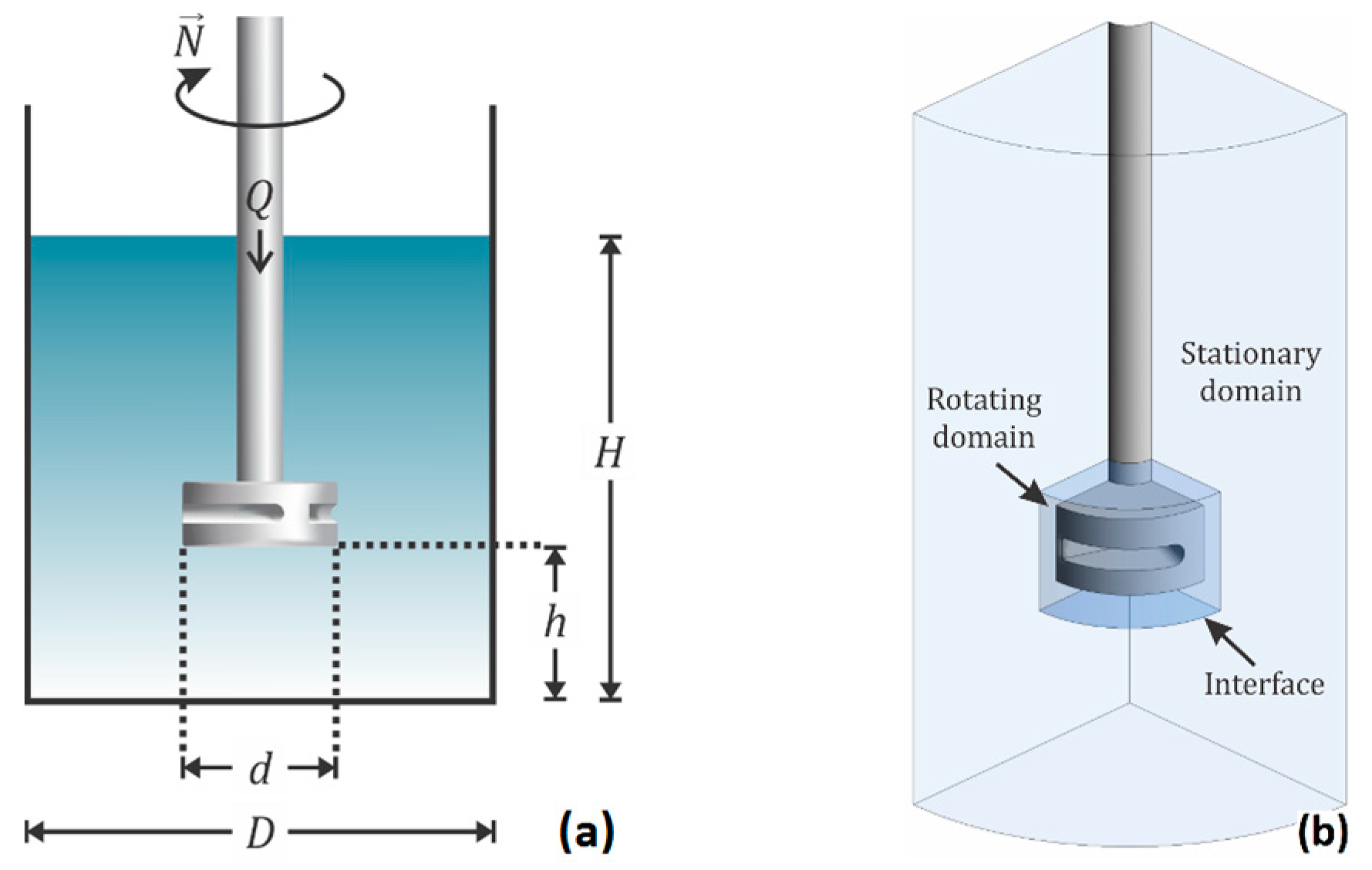
2.4. Boundary and Initial Conditions
2.5. Solution
2.6. Experimental Procedure
3. Results and Discussion
3.1. Validation
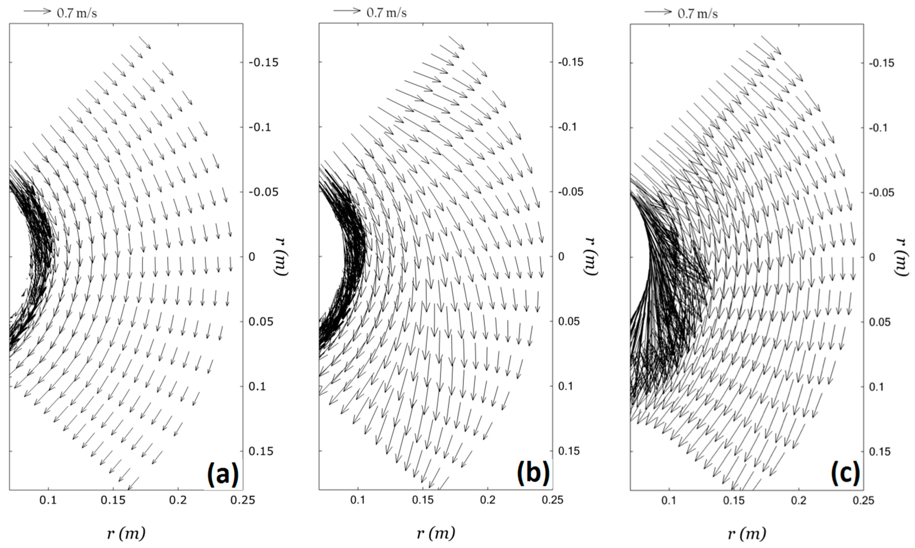
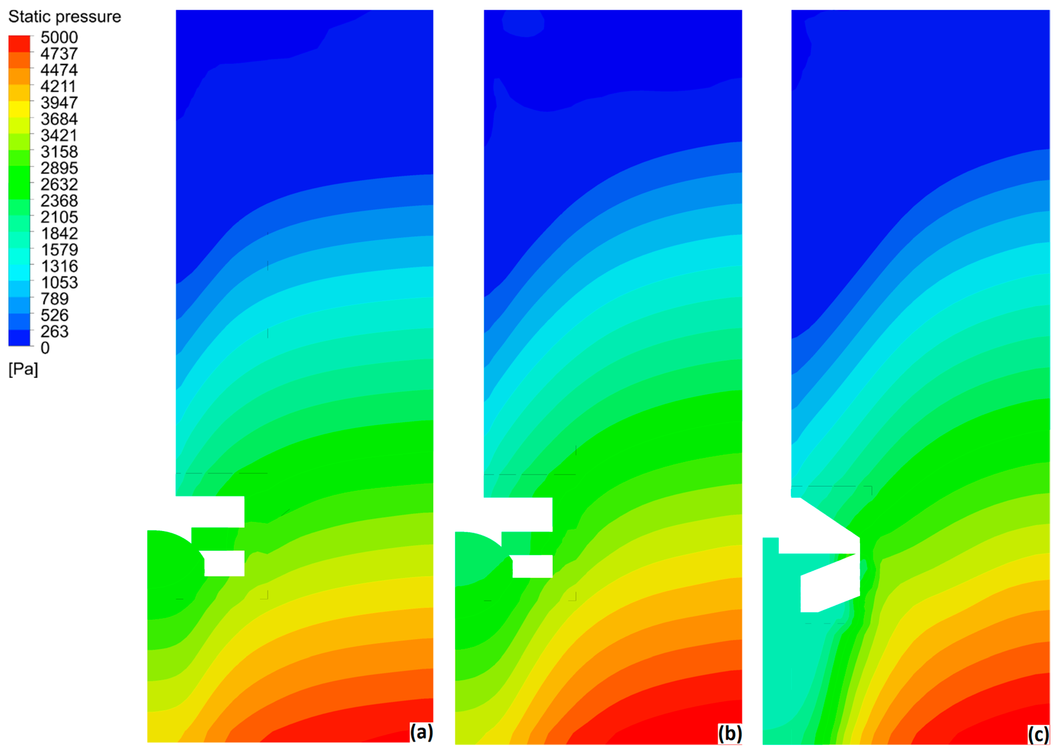
3.2. Process Analysis
4. Conclusions
Acknowledgments
Author Contributions
Conflicts of Interest
Abbreviations
| List of symbols | ||
| Interfacial area concentration | ||
| inverse Prandtl number for turbulent kinetic energy | ||
| Swirl modification constant | ||
| inverse Prandtl number for dissipation rate of turbulent kinetic energy | ||
| Drag coefficient | ||
| Drag function | ||
| RNG k-ε model constant | ||
| RNG k-ε model constant | ||
| RNG k-ε model constant | ||
| Turbulent dispersed model constant | ||
| Turbulent dispersed model constant | ||
| Impeller diameter | ||
| Ladle diameter | ||
| Bubble diameter | ||
| Swirl modification function | ||
| Momentum exchange between phases | ||
| Gravity acceleration | ||
| Generation of turbulent kinetic energy | ||
| Distance from bottom to impeller line | ||
| Height of liquid | ||
| Turbulent kinetic energy | ||
| Exchange coefficient between phase and phase | ||
| Angular velocity | ||
| Pressure | ||
| Gas flow rate | ||
| Radial position vector | ||
| Coriolis and centrifugal forces in the rotating frame of reference | ||
| Term from RNG k-ε model | ||
| Reynolds number | ||
| Strain rate magnitude | ||
| Strain rate tensor | ||
| Time | ||
| Velocity | ||
| Greek symbols | ||
| Volume fraction | ||
| RNG k-ε model constant | ||
| Dissipation rate of turbulent kinetic energy | ||
| RNG k-ε model relation | ||
| RNG k-ε model constant | ||
| Drag modification of Brucato’s model | ||
| Viscosity | ||
| Source term of turbulent kinetic energy | ||
| Source term of dissipation rate of turbulent kinetic energy | ||
| Density | ||
| Particle relaxation time | ||
| Characteristic swirl number | ||
| Subscripts | ||
| Liquid phase | ||
| Gas phase | ||
| Turbulent | ||
| Effective | ||
References
- Ramos Gomez, E.; Zenit, R.; González Rivera, C.; Trápaga, G.; Ramírez Argáez, M.A. Mathematical Modeling of Fluid Flow in a Water Physical Model of an Aluminum Degassing Ladle Equipped with Impeller-Injector. Metall. Mater. Trans. B 2013, 44, 423–435. [Google Scholar] [CrossRef]
- Lane, G.L.; Schwarz, M.P.; Evans, G.M. Numerical modeling of gas-liquid flow in stirred tanks. Chem. Eng. Sci. 2005, 60, 2203–2213. [Google Scholar] [CrossRef]
- Deen, N.G.; Solberg, T.; Hjertager, B.H. Flow generated by an aerated Rushton impeller: Two-phase PIV experiments and numerical simulations. Can. J. Chem. Eng. 2002, 80, 638–652. [Google Scholar] [CrossRef]
- Johansen, S.T.; Boysan, F. Fluid Dynamics in Bubbled Stirred Ladles. Part II: Mathematical Modeling. Metall. Trans. B 1988, 19, 755–764. [Google Scholar] [CrossRef]
- Ilegbusi, O.J.; Szekely, J. The Modeling of Gas-Bubble Driven Circulations Systems. ISIJ Int. 1990, 30, 731–739. [Google Scholar] [CrossRef]
- Johansen, S.T.; Fredriksen, A.; Rasch, B. Particle Flotation to Bubbles in Rotor-Stirred reactors for Melt Treatment. In Light Metals, the Minerals, Metals and Materials Society; TMS: Las Vegas, NV, USA, 1995; pp. 1203–1206. [Google Scholar]
- Hop, B.; Johansen, S.T.; Rasch, B. A 3D Numerical Model for Removal of Inclusions to Gas Bubbles. In Light Metals, the Minerals, Metals and Materials Society; TMS: Anaheim, CA, USA, 1996; pp. 647–656. [Google Scholar]
- Maniruzamman, M.; Makhlouf, M. Mathematical Modeling and Computer Simulation of the Rotating Impeller Particle Flotation Process: Part II. Particle Agglomeration and Flotation. Metall. Mater. Trans. B 2002, 33, 305–314. [Google Scholar] [CrossRef]
- Maniruzamman, M.; Makhlouf, M. Mathematical Modeling and Computer Simulation of the Rotating Impeller Particle Flotation Process: Part I. Fluid Flow. Metall. Mater. Trans. B 2002, 33, 297–303. [Google Scholar] [CrossRef]
- Warke, V.S.; Tryggvason, G.; Makhlouf, M.M. Mathematical Modeling and Computer Simulation of Molten Metal Cleansing by the Rotating Impeller Degasser: Part I. Fluid Flow. J. Mater. Process. Technol. 2005, 168, 112–118. [Google Scholar] [CrossRef]
- Warke, V.S.; Shankar, S.; Makhlouf, M.M. Mathematical Modeling and Computer Simulation of Molten Metal Cleansing by the Rotating Impeller Degasser: Part II. Removal of hydrogen gas and solid particles. J. Mater. Process. Technol. 2005, 168, 119–126. [Google Scholar] [CrossRef]
- Mirgaux, A.; Ablitzer, D.; Waz, E.; Bellot, J.E. Mathematical modeling and computer simulation of molten aluminum purification by flotation in stirred reactor. Metall. Mater. Trans. B 2009, 40, 363–375. [Google Scholar] [CrossRef]
- Hop, B.; Frisvold, F.; Rasch, B.; Johansen, S.T. The fluid mechanics in the H110 Hycast reactor. In Light Metals, the Minerals, Metals and Materials Society; TMS: Orlando, FL, USA, 1997; pp. 837–841. [Google Scholar]
- Dong, L.; Johansen, S.T.; Engh, T.A. Flow induced by an impeller in an unbaffled tank—II. Numerical Modeling. Chem. Eng. Sci. 1994, 49, 3511–3518. [Google Scholar] [CrossRef]
- Mancilla, E.; Cruz-Mendez, W.; Garduño, I.; González-Rivera, C.; Ramírez-Argáez, M.; Ascanio, G. Comparison of the hydrodynamic performance of rotor-injector devices in a water physical model of an aluminum degassing ladle. Chem. Eng. Res. Des. 2016, 118, 158–169. [Google Scholar] [CrossRef]
- Hernández-Hernández, M.; Camacho-Martínez, J.L.; González-Rivera, C.; Ramirez-Argáez, M.A. Impeller Design Assisted by Physical Modeling and Pilot Plant Trials. J. Mater. Process. Technol. 2016, 236, 1–8. [Google Scholar] [CrossRef]
- Brucato, A.; Grisafi, F.; Montante, G. Particle drag coefficients in turbulent fluids. Chem. Eng. Sci. 1998, 53, 3295–3314. [Google Scholar] [CrossRef]
- Schiller, L.; Naumann, Z. A drag coefficient correlation. Z. Ver. Deutsch. Ing. 1935, 77, 51. [Google Scholar]


| Characteristic | Description |
|---|---|
| Fluids | Incompressible and Newtonian, water and air |
| Flow regime | Turbulent (Re = 1,160,000) |
| Rotating speed () | 400 rpm |
| Gas flow rate () | 10 L/min |
| Ladle diameter () | 0.5 m |
| Impeller diameter () | 0.166 m |
| Height of liquid () | 0.5 m |
| Distance from bottom to impeller line () | 0.166 m |
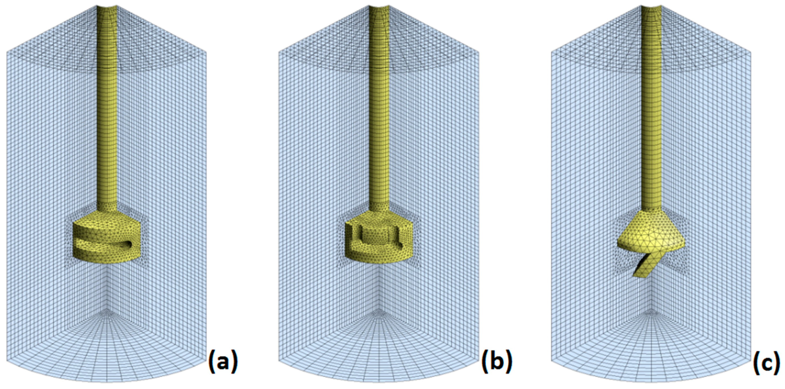
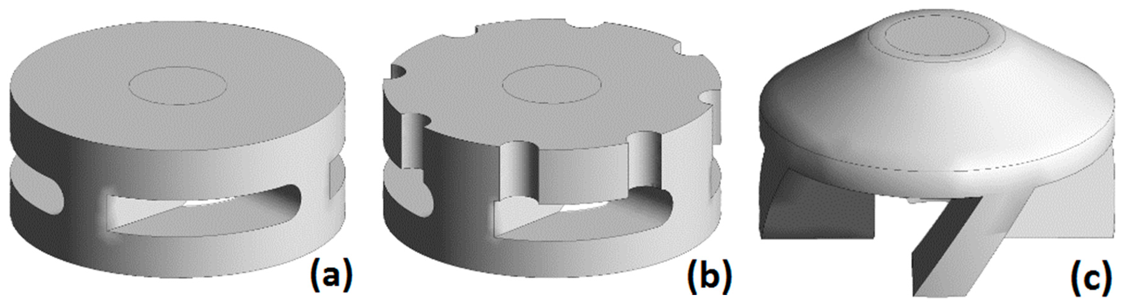
| Impeller design | Commercial designs A and B and a new design C (Figure 2) |
| Geometry | Elements | Total | |
|---|---|---|---|
| Hexahedric | Tetrahedric | ||
| Impeller design A | 29,270 | 34,030 | 63,300 |
| Impeller design B | 29,270 | 31,610 | 60,880 |
| Impeller design C | 31,520 | 21,000 | 52,520 |
© 2017 by the authors. Licensee MDPI, Basel, Switzerland. This article is an open access article distributed under the terms and conditions of the Creative Commons Attribution (CC BY) license (http://creativecommons.org/licenses/by/4.0/).
Share and Cite
Abreu-López, D.; Amaro-Villeda, A.; Acosta-González, F.A.; González-Rivera, C.; Ramírez-Argáez, M.A. Effect of the Impeller Design on Degasification Kinetics Using the Impeller Injector Technique Assisted by Mathematical Modeling. Metals 2017, 7, 132. https://doi.org/10.3390/met7040132
Abreu-López D, Amaro-Villeda A, Acosta-González FA, González-Rivera C, Ramírez-Argáez MA. Effect of the Impeller Design on Degasification Kinetics Using the Impeller Injector Technique Assisted by Mathematical Modeling. Metals. 2017; 7(4):132. https://doi.org/10.3390/met7040132
Chicago/Turabian StyleAbreu-López, Diego, Adrián Amaro-Villeda, Francisco A. Acosta-González, Carlos González-Rivera, and Marco A. Ramírez-Argáez. 2017. "Effect of the Impeller Design on Degasification Kinetics Using the Impeller Injector Technique Assisted by Mathematical Modeling" Metals 7, no. 4: 132. https://doi.org/10.3390/met7040132
APA StyleAbreu-López, D., Amaro-Villeda, A., Acosta-González, F. A., González-Rivera, C., & Ramírez-Argáez, M. A. (2017). Effect of the Impeller Design on Degasification Kinetics Using the Impeller Injector Technique Assisted by Mathematical Modeling. Metals, 7(4), 132. https://doi.org/10.3390/met7040132