Mathematical Modeling of the Concentrated Energy Flow Effect on Metallic Materials

Abstract

Numerous processes take place in materials under the action of concentrated energy flows. The most important ones include heating together with the temperature misdistribution throughout the depth, probable vaporization on the surface layer, melting to a definite depth, and hydrodynamic flotation; generation of thermo-elastic waves; dissolution of heterogeneous matrix particles; and formation of nanolayers. The heat-based model is presented in an enthalpy statement involving changes in the boundary conditions, which makes it possible to consider melting and vaporization on the material surface. As a result, a linear dependence of penetration depth vs. energy density has been derived. The model of thermo-elastic wave generation is based on the system of equations on the uncoupled one-dimensional problem of dynamic thermo-elasticity for a layer with the finite thickness. This problem was solved analytically by the symbolic method. It has been revealed for the first time that the generated stress pulse comprises tension and compression zones, which are caused by increases and decreases in temperature on the boundary. The dissolution of alloying elements is modeled on the example of a titanium-carbon system in the process of electron beam action. The mathematical model is proposed to describe it, and a procedure is suggested to solve the problem of carbon distribution in titanium carbide and liquid titanium-carbide solution in terms of the state diagram and temperature changes caused by phase transitions. Carbon concentration vs. spatial values were calculated for various points of time at diverse initial temperatures of the cell. The dependence of carbon particle dissolution on initial temperature and radius of the particle were derived. A hydrodynamic model based on the evolution of Kelvin-Helmholtz instability in shear viscous flows has been proposed to specify the formation of nanostructures in materials subjected to the action of concentrated energy flows. It has been pointed out for the first time that, for certain parameters of the problem, that there are two micro- and nanoscale peaks in the relation of the decrement to the wavelength of the interface disturbance.

1. Introduction

At present the flows of concentrated energy find wide application in processing surfaces of various materials [1,2,3,4,5]. For instance, low-energy, high-current electron beams with durations up to milliseconds, which is used for strengthening the surface layer [2], smoothing the surface relief [3,5], and forming micro- and nano-crystalline grains [4,5,6]. The advantages of electron beam treatment mainly include [7]: extensive control over modes and fine adjustment of heat flow; suitable for both metals and non-metals; high efficiency coefficient (up to 98%); and automation of process. Combined treatment is a promising procedure of surface modification. This implies the use of heterogeneous plasma flows generated by electric explosion of conductors with the subsequent exposure to electron beams [8,9,10]. The surfaces modified by above method have quite unique characteristics, for example, the wear resistance properties after surfaces modification increase by 7.5 times [8,9,10]. Wide-scale research is required to determine the relationship of processing parameters and properties. To reduce the time needed for this kind of research some mechanisms are to be developed, as well as some mathematical models are necessary to specify the processes of combined treatment: heat transfer to the target, generation of stress waves, structural and phase transformations in liquid and solid states, and hydrodynamic flows in the molten layer.

The first mathematical models describing heat and thermo-elastic processes under the action of electron beams were proposed almost 20 years ago [11,12]. Leyvi et al. [13] analyzed the present day experimental and theoretical studies focused on modification of engineering materials by intense flows of charged particles and plasma. They comprise: kinetic equation to simulate the interaction of concentrated energy flows with the material, continuum mechanics equations (variation of mass, pulse, and energy) for target material and the wide-range equation of state.

Researchers [14,15,16] took a close look at the works linked with simulations of heat processes with evaporation. Models and software complexes are developed, which can provide comprehensive data for working out certain technologies. The problems of heat impact on laser emission target were investigated [14], taking into account evaporation and vapor dissemination. It is a complex problem of gas-dynamic flow in the flame of evaporated substances and thermal processes. However, the study was unable to demonstrate how to monitor the melt front. Bleykher et al. [15] modeled the field of temperatures and evaporation rates under magnetron action on the target. The field of temperatures and evaporation rates are calculated when finding solution of boundary problem, thermal conductivity equation, and boundary conditions, with the evaporation rate considered. The rate of evaporation here is determined relying on Hertz-Knudsen equation, although processes occurring in the target were not analyzed. The authors [16] dealt with the effect of charged particles on the target and suggested a model, which rests on kinetic equation for particles, continuum mechanics equation, and the wide-range equation of state. However, no correlation between penetration depth and beam parameters was found. Therefore, it makes sense to use a simplified model [17], which provides a quite correct description of temperature fields in the target under the action of electron beams and allows the determination of the penetration depth.

Some authors [13,18,19] have attempted to develop models for the stress state determination under concentrated energy flows. They referred to complex behavioral models of the continuum, and dynamic problems for layers with finite thickness have a computational solution. It is possible to model the definite dissemination of stress waves, but wave reflection can be studied in detail only on the basis of the analytical solution of the simplified model of disconnected thermo-elasticity [20].

Combined treatment implies, first, the injection of carbon powder into molten titanium by means of the heterogeneous plasma flow, and second, the impact of electron beam on the heterogeneous titanium-carbon particles system. Under the action of electron beams on the heterogeneous titanium mixture, melting occurs, but carbon particles are in a solid state, as the fusion temperature of carbon is 3550 °C. Whether carbon particles dissolve over the time of the electron beam impact (100 µm), a homogenous layer of titanium carbide will be formed. As a consequence, a mathematical model, which allows the determination of the electron beam parameters, is required to further synthesize a homogenous layer of carbide. The problem of iso-thermal dissolution of a new phase spherical center within the diffusion model has been solved [21], and was confined to the Stefan problem for the diffusion equation in the zone, on the flexible boundary of which the conditions of mass balance are satisfied. When carbon reacts with titanium, the temperature changes as heating and cooling occur in the process of electron beam impact and exothermic reaction. Diffusion and temperature problems are solved simultaneously in [22,23] in accordance with diverse spatial and temporal scales. This approach is quite complex since it necessitates consideration of heat release in the thermo-conductivity equation. The method stated in combustion theory [24], and applied further in [25,26], was used for consideration of the changing temperature. It relies on the heat-balance equation for a cell on the whole; that is, there is no change in temperature along the spatial value. The first phase of experimental interaction in the system Ti-С and physical and chemical processes taking place in carbon fusion have been investigated [27], and the double-wave structure of wave transformation was proved experimentally. A mathematical model of carbon distribution in titanium carbide and liquid titanium-carbon solution was suggested [28], which, taking into account the diagram of states and phase transitions, result from temperature changes. The authors of this work suggested a framework implying the determination of such process characteristics, which allow the understanding of the controlled process parameters (e.g., energy density of electron beam, pulse duration, pulse repetition, etc.) on the outcomes of experiments. For instance, whether a particle of carbon dissolves in liquid titanium exposed to electron beam. In this case it is quite reasonable to address only to diffusion problem for homogenous temperature field, which can vary over time due to heat of chemical reactions and heat removal. Solution of this problem helps to realize the reason for generation of homogenous titanium layers exposed to heterogeneous plasma flows and processed further by low-energy high-current electron beam [8,9].

Numerous publications emphasize the interest of researchers in development of mathematical models describing nano-structures under the action of concentrated energy flows [29,30,31,32,33,34,35,36,37,38,39]. These models are based mainly on computer simulation of processes, going with the development of nano-structural states. The researchers [29,30] speculated that nano-structural state evolves together with the growing hydrodynamic instability in shear-related motion of liquid layers, one of them is viscous. In this case the dispersion equation is considered as a quartic algebraic equation with complex variables. It is rather complicated to analyze the parameters, so decrement vs. wavenumber was assessed numerically. The wavelength agreeing with the peak of the decrement is the most instable; therefore, this wave preserves its length, making its observation possible in the experiment. Two peaks were revealed in decrement vs. wavelength correlation. Approximation of short waves is used in [39], and a simplified dispersion equation is derived. The values of wavelengths were determined for two peaks on the base of this equation. This fact is of significant importance for parameterization of experimental outcomes. This work is focused on derivation and analysis of the dispersion equation for finite layers.

2. Mathematical Models of Electron-Beam Effect on Metallic Materials

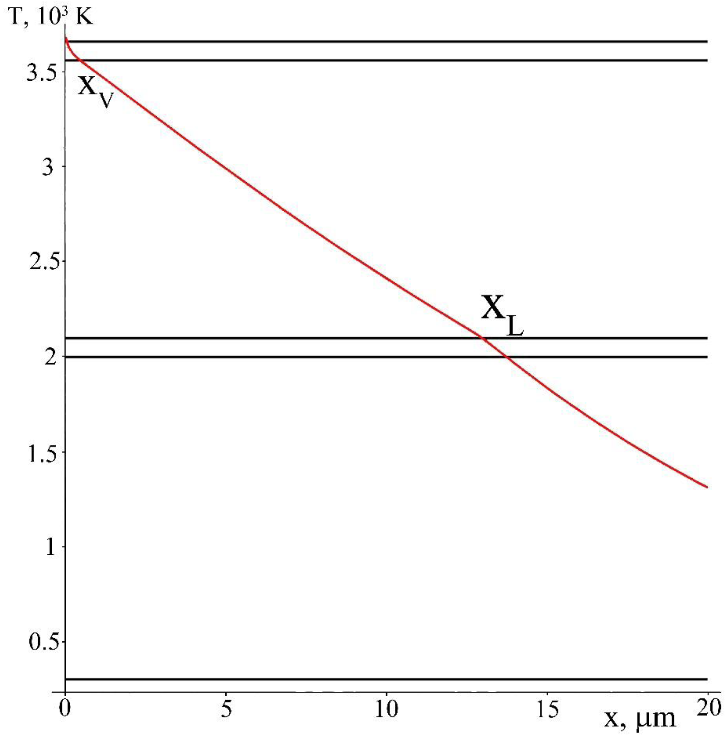
2.1. Thermal Model

Let us consider the impact of the electron beam with the surface energy density E_S on a flat plate with the thickness l. As we are interested in the distribution of temperature over the depth of the sample, we confine ourselves to solving the one-dimensional problem of thermal conductivity. The x axis is directed inside the plate. The surface х = 0 is affected by the electron current during the period of time t₀, and there is no heat flow on the back side of the plate х = l. The equation of thermal conductivity is written in an enthalpy statement in order to take into consideration the phase transformations on the boundary:

$$\frac{\partial H}{\partial t}=\frac{\partial }{\partial x}\left(\mathsf{\lambda }\frac{\partial T}{\partial x}\right)$$

(1)

where enthalpy is:

$$H\left(T\right)={\displaystyle \underset{0}{\overset{T}{\int }}C\left(T\right)\mathsf{\rho }\left(T\right)dT},C\left(T\right)\mathsf{\rho }\left(T\right)=\{\begin{array}{l}{C}_S{\mathsf{\rho }}_S,T<T_S\\ L_L{\mathsf{\rho }}_L/\Delta T_1,T_S<T<T_L\\ C_L{\mathsf{\rho }}_L,T_L<T<T_V\\ L_V{\mathsf{\rho }}_L/\Delta T_2,T_V<T\end{array}$$

(2)

where C is specific heat; ρ—density; T—temperature; t—time; λ—thermal conductivity, for which:

$$\mathsf{\lambda }=\{\begin{array}{l}{\mathsf{\lambda }}_S,T<T_S\\ {\mathsf{\lambda }}_S+\frac{{\mathsf{\lambda }}_L-{\mathsf{\lambda }}_S}{\Delta T_1}\left(T-T_L\right),T_S<T<T_L\\ {\mathsf{\lambda }}_L,T_L<T<T_V\\ {\mathsf{\lambda }}_L+\frac{{\mathsf{\lambda }}_V-{\mathsf{\lambda }}_L}{\Delta T_2}\left(T-T_V\right),T_V<T\end{array}$$

(3)

Here indices S, L, and V refer to solid, liquid, and gas phases; L_L and L_V are latent heats of melting and vaporization. We suppose ∆T₁ = 100 K; ∆T₂ = 100 K. The solution of Equation (1) requires setting initial and boundary conditions. The initial condition is dependent on the constant temperature, which equals to 300 К.

$$T\left(0,x\right)=T_0,0<x<l$$

(4)

The boundary condition at х = l is written as follows:

$$\frac{\partial T\left(t,l\right)}{\partial x}=0,t>0$$

(5)

Mixed boundary conditions at х = 0 are used to take into account the effect of vaporization, and a heat flow is set till the start of vaporization:

$$\mathsf{\lambda }\frac{\partial T\left(0,t\right)}{\partial x}=-\frac{E_S}{t_0},0<t<t_1$$

(6)

where t₁—time when boundary conditions is changed, and it is determined on assumption that the enthalpy on the surface is similar to the vaporization enthalpy at normal pressure, i.e., it results from the equation H(0,t₁) = H_V. Over the period from t₁ to the completion of the electron beam impact (t₀) energy is supplied to the system and consumed for vaporization and emission of the evaporated substance. At these points the enthalpy on the vapor-liquid boundary is constant and equals to the heat of vaporization H_V. This boundary moves into the zone of the plate (up to 1 μm), but we disregard this shift and suppose the boundary condition is as follows:

$$H\left(0,t\right)=H_V,t_1<t<t_0$$

(7)

As soon as the pulse impact is over, vapor contacts with the plate surface; since the time of vapor emission is several hundreds of microseconds, the temperature of the sample surface is equated to that of vaporization:

$$T\left(0,t\right)=T_V,t_0<t<t_2$$

(8)

After completion of the vapor contact with the surface, its temperature can vary in the absence of heat exchange, therefore, the condition of heat exchange is stated as:

$$\frac{\partial T\left(t,0\right)}{\partial x}=0,t>t_2$$

(9)

Thermal and physical characteristics of commercially pure titanium [40,41,42]: T_S = 1998 К; L_m = 304 kJ/kg; T_V = 3560 К; L_V = 8900 kJ/kg; ρ_S = 4.5 × 10³ kg/m³; ρ_L = 4.1 × 10³ kg/m³; C_S = 318 J/(kg·К); C_L = 400 J/(kg·К); λ_S = 25 W/(m·К); λ_L = 10 W/(m·К). The problem was solved numerically (1)–(9) for λ_L, varying in the range from 20–40 W/(m·К). The coefficient of thermal conductivity of the liquid titanium was selected on assumption that the estimated and experimental values of the penetration depth are concurrent.

To calculate time t₂ we integrate the Equation (1) according to х from zero to l:

$$\frac{\partial W}{\partial t}=-\mathsf{\lambda }\frac{\partial T\left(t,0\right)}{\partial x},W\left(t\right)={\displaystyle \underset{0}{\overset{l}{\int }}H\left(t,x\right)dx}$$

(10)

The Equation (10) we integrate according to time from zero to t₂:

$$W(t_2)-W(0)=-{\displaystyle \underset{0}{\overset{t_1}{\int }}\mathsf{\lambda }\frac{\partial T(t,0)}{\partial x}}dt-{\displaystyle \underset{t_1}{\overset{t_0}{\int }}\mathsf{\lambda }\frac{\partial T(t,0)}{\partial x}dt}-{\displaystyle \underset{t_0}{\overset{t_2}{\int }}\mathsf{\lambda }\frac{\partial T(t,0)}{\partial x}dt}$$

(11)

We obtain an expression for each summand in the right part of Equation (11):

$$\begin{gathered} -{\displaystyle \underset{0}{\overset{t_1}{\int }}\mathsf{\lambda }\frac{\partial T(t,0)}{\partial x}}dt=\frac{E_S{t}_1}{t_0} \\ -{\displaystyle \underset{t_1}{\overset{t_0}{\int }}\mathsf{\lambda }\frac{\partial T(t,0)}{\partial x}}dt=-(T_V-T_2){\displaystyle \underset{t_1}{\overset{t_0}{\int }}\frac{{\mathsf{\lambda }}_V}{x_V}}dt \\ -{\displaystyle \underset{t_0}{\overset{t_2}{\int }}\mathsf{\lambda }\frac{\partial T(t,0)}{\partial x}}dt=-(T_1-T_V){\displaystyle \underset{t_0}{\overset{t_2}{\int }}\frac{{\mathsf{\lambda }}_L}{x_L}}dt \end{gathered}$$

(12)

Here x_V(t) and x_L(t) are computable dependencies of vaporization front coordinates and melting on time, which are given in Figure 1.

The system is supplied with the energy per a unit of area W(t₂) − W(0) = E_S; taking into consideration Equations (12). Equation (11) is written as follows:

$$E_S\left(1-\frac{t_1}{t_0}\right)+(T_V-T_2){\displaystyle \underset{t_1}{\overset{t_0}{\int }}\frac{{\mathsf{\lambda }}_V}{x_V}dt+(T_1-T_V)}{\displaystyle \underset{t_0}{\overset{t_2}{\int }}\frac{{\mathsf{\lambda }}_L}{x_L}dt}=0$$

(13)

On the basis of Equation (13) we determine t₂. The temperature was calculated by means of the implicit first-order difference scheme with respect to time and by the second-order scheme with respect to space. The time increment is 1 μs, and the space increment is 0.1 μm. The obtained algebraic system of equations was solved by the double-sweep method. The thickness of the plate l is set to 600 μm; this quite large thickness can provide results similar to those of an infinitely thick plate over the time, up to 2000 μs [11,12,13,14,15,16,17,40]. The depths of penetration in diverse process conditions of electron beam treatment are given in

Table 1. The dependence of penetration depth on energy density.

ES, J/cm2	t0, μs	hmelt, μm
		Experimental	Estimated
18	50	6	7
21	50	8	8
25	50	13	15
45	100	31.1	31.2
50	100	36	35.0
60	100	50.1	50

. It is seen that estimated and experimental values are quite identical. In accordance to the data in Table 1 the dependence of penetration depth on the surface energy density is linear.

The processes of vaporization are quite irrelevant at energy density ranging from 10–30 J/cm² because temperature on the surface does not reach that of vaporization. As soon as pulse action is completed there is a sharp drop in temperature on the surface, therefore, the penetration depth is small ~10 μm. At Es > 30 J/cm² temperature on the surface reaches the temperature of vaporization. A layer of vapor generated over this process creates a heat buffer, as stated above. As a result, temperature on the surface is quite constant from time T = T_V to the time when pulse action is completed. This period of time is dependent on energy density. The higher energy density is the longer temperature on the surface is constant. As a consequence, penetration depth increases. The derived dependence of penetration depth on energy density can provide a basis for choosing proper modes of low-energy high-current electron beam treatment.

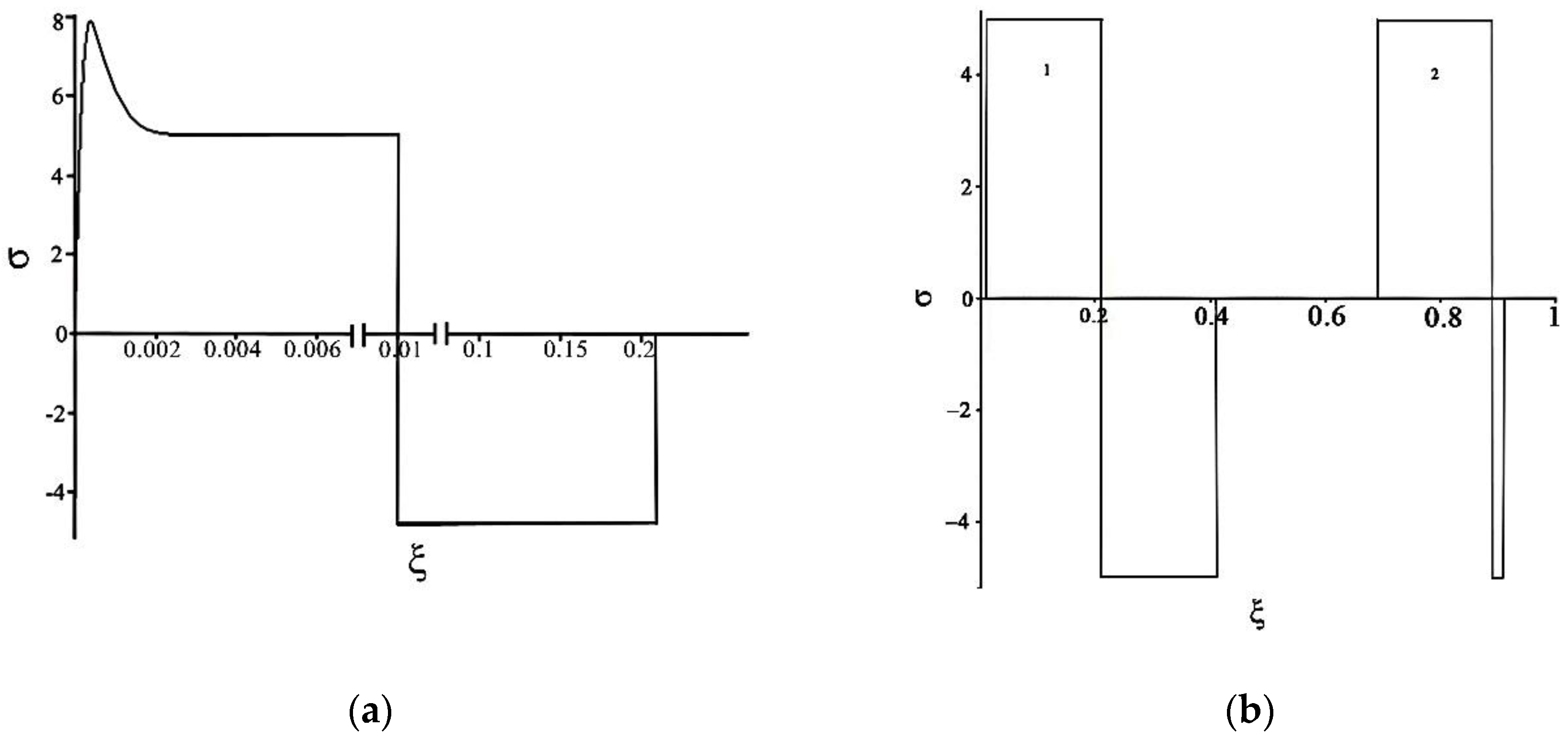
2.2. Model of Thermoelastic Waves Generation

Generation of the thermoelastic waves is a principal problem to be solved for modelling the processes caused by the concentrated energy flows. An attempt to model a thermal situation relying on heat transfer from the inner heat source and generation of thermoelastic waves has been made in [18,19,20,43], where the bipolarity of the thermoelastic wave was modeled numerically. However, the mechanism of origination, that is, the relationship arising from compression and tension to the zones of heating and cooling was not identified.

In this paper the causes and the mechanism of bipolar thermoelastic wave generation were revealed on the basis of an analytical solution of the thermoelastic problem for the layer with a finite thickness when heating the surface, the stress states close to the back and front surfaces were determined as well.

We consider the problem of thermal stresses for a stress-free flat sample with the thickness, which is subject to the heat flow impact. We set thermal conditions as temperature heating. The axis is perpendicular to the surface of the sample; the other two axes are in the plane of energy flow impact. The plane is referred to as a front surface, and the plane is a back one. We assume that the energy flow is homogenous in the cross-section, therefore, one-dimensional statement of problem is selected, that is, all functions are dependent on the only one spatial variable, where we consider the one-axial stress-strain state with non-zero components of the strain tensors. To state the mathematical problem we use the equations of motion and thermal conductivity, as well as the Duhamel-Neumann relation, the so called dynamic problem of the disconnected thermo-elastisity [31]:

$$\mathsf{\rho }\frac{{\partial }^{2}u}{\partial t^2}=\frac{\partial {\mathsf{\sigma }}_x}{\partial x},\frac{1}{\mathsf{\chi }}\frac{\partial T}{\partial t}=\frac{{\partial }^{2}T}{\partial x^2},{\mathsf{\sigma }}_x=\mathsf{\rho }{c}^2\frac{\partial u}{\partial x}-\mathsf{\gamma }T$$

(14)

Here, ρ, χ are the density and thermal diffusivity of the material, $c=\sqrt{(2\mathsf{\mu }+\mathsf{\lambda })/\mathsf{\rho }}$ is the rate of longitudinal wave propagation, $\mathsf{\gamma }=(3\mathsf{\lambda }+2\mathsf{\mu }){\mathsf{\alpha }}_t$ is the coefficient of the thermoelastic coupling, λ, μ are the Lame coefficients, α_t is the coefficient of linear expansion, u = u(t,x) is the component of the displacement vector, and T = T(t,x) is the temperature distribution.

A thermal situation at the front surface under the action of energy flows can be written as temperature heating:

$$T(t,0)={\mathsf{\Psi }}_0(t)$$

(15)

We set ${\mathsf{\Psi }}_0(t)$ as a trapezoid. In this case the surface temperature increases in the range from zero to T₀ over the period of time t₁, it is constant for the period of time t₂, and goes down from T₀ to zero over the period of time t₃. The right part Equation (15) is written as follows:

$${\mathsf{\Psi }}_0(t)=\frac{t}{t_1}(H(t)-H(t-t_1))+(H(t-t_1)-H(t-t_1-t_2))-\frac{t-t_1-t_2}{t_3}(H(t-t_1-t_2)-H(t-t_1-t_2-t_3))$$

(16)

where H(t) is the Heaviside step function.

In Equation (15) the initial conditions are generalized by taking Equation (16) into consideration, and the following problems are solved for these conditions: at $l_0=\infty$: Danilevskaya problem—momentary growth of temperature ($t_1=0,t_2=\infty ,t_3=0$), the problem with the finite time of temperature increase up to the certain value (t₁—finite, $t_2=\infty$), and the case of the increase and decline of temperature over the same time (t₁ = t₃, t₂ = 0) [44].

Without any regard to the energy flow we assume that a sample is not fixed in the plane of the flow action. The boundary conditions for the stress equal to zero:

$${\mathsf{\sigma }}_x(t,0)={\mathsf{\sigma }}_x(t,l_0)=0$$

(17)

The initial conditions of the problem:

$${\mathsf{\sigma }}_x(0,x)=0,T(0,x)=T_2,\frac{\partial {\mathsf{\sigma }}_x}{\partial t}(0,x)=0$$

(18)

The stated problem has two typical spatial scales: dynamic, equal to the thickness of the sample l₀ = ~1 mm, and thermal—l_T = ~10 μm. Therefore, the equation of dynamics is considered in the range from zero to l₀, whereas the equation of thermal conductivity is considered on the semi-finite line with a zero temperature at infinity.

The mathematical problem in non-dimensional variables Equations (14)–(18) is written as follows:

$$\begin{array}{l}\ddot{\mathsf{\sigma }}+\ddot{\mathsf{\theta }}={\mathsf{\sigma }}^{″},0<\mathsf{\xi }<1,\mathsf{\tau }>0;\mathsf{\alpha }\dot{\mathsf{\theta }}={\mathsf{\theta }}^{″},\mathsf{\xi }>0,\mathsf{\tau }>0\\ \mathsf{\theta }(\mathsf{\tau },0)={\mathsf{\Psi }}_0(\mathsf{\tau }),\mathsf{\theta }(\mathsf{\tau },\infty )=0;\\ \mathsf{\sigma }(\mathsf{\tau },0)=\mathsf{\sigma }(\mathsf{\tau },1)=0;\mathsf{\sigma }(0,\mathsf{\xi })=\mathsf{\sigma }(0,\mathsf{\xi })=\dot{\mathsf{\sigma }}(0,\mathsf{\xi })=0.\end{array}$$

(19)

The non-dimensional variables are set according to formulae:

$$\mathsf{\xi }=\frac{x}{l_0},\mathsf{\tau }=\frac{tc}{l_0},\mathsf{\sigma }=\frac{{\mathsf{\sigma }}_x}{\mathsf{\gamma }{T}_0},\mathsf{\theta }=\frac{T}{T_0},\mathsf{\alpha }=\frac{l_{0}c}{\mathsf{\chi }},{\mathsf{\tau }}_1=\frac{t_{1}c}{l_0},{\mathsf{\tau }}_2=\frac{t_{2}c}{l_0},{\mathsf{\tau }}_3=\frac{t_{3}c}{l_0}$$

(20)

To solve the problem Equation (19) the Laplace transform is used. For the images a system of differential equations is written with the corresponding boundary conditions:

$$\begin{array}{l}{{\mathsf{\sigma }}_L}^{″}(p,\mathsf{\xi })-p^2{\mathsf{\sigma }}_L(p,\mathsf{\xi })=p^2{\mathsf{\theta }}_L(p,\mathsf{\xi }),{\mathsf{\sigma }}_L(p,0)={\mathsf{\sigma }}_L(p,1)=0\\ {{\mathsf{\theta }}_L}^{″}(p,\mathsf{\xi })-b^2{\mathsf{\theta }}_L(p,\mathsf{\xi })=0,\mathsf{\theta }(p,0)=\mathsf{\Psi }(p),{\mathsf{\theta }}_L(p,\infty )=0\end{array}$$

(21)

where $b^2=\mathsf{\alpha }p$ and ${\mathsf{\Psi }}_0(p)$ is the Laplace transform of the function ${\mathsf{\Psi }}_0(\mathsf{\tau })$ set according to Equation (16). The solution of the problem Equation (21) is written as follows:

$${\mathsf{\theta }}_L(p,\mathsf{\xi })=\frac{\mathsf{\Psi }(p)}{b}\exp (-b\mathsf{\xi })$$

(22)

$${\mathsf{\sigma }}_L(p,\mathsf{\xi })=\frac{p\mathsf{\Psi }(p)}{(p-\mathsf{\alpha })}\left(W(\mathsf{\xi })-W(1)\frac{\sinh (p\mathsf{\xi })}{\sinh (p)}\right)$$

(23)

where:

$$\begin{array}{l}\mathsf{\Psi }(p)=\frac{1}{p^2}\left(\frac{1-\exp (-p{\mathsf{\tau }}_1)}{{\mathsf{\tau }}_1}-\exp (-p({\mathsf{\tau }}_1+{\mathsf{\tau }}_2))\frac{1-\exp (-p{\mathsf{\tau }}_3)}{{\mathsf{\tau }}_3}\right)\\ W(\mathsf{\xi })=\exp (-p\mathsf{\xi })-\exp (-b\mathsf{\xi })\end{array}$$

(24)

The first summand in Equation (23) is an image of the stress in the wave, generated via temperature heating, and the second summand represents the superposition of the straight wave and the wave reflected from the back and front surfaces:

$${\mathsf{\sigma }}_L(p,\mathsf{\xi })={\mathsf{\sigma }}_{L\infty }(p,\mathsf{\xi })+{\mathsf{\sigma }}_{L\leftarrow }(p,\mathsf{\xi })+{\mathsf{\sigma }}_{L\to }(p,\mathsf{\xi })$$

(25)

The expression below is obtained according to the sum of infinite geometric sequence formula:

$$\begin{array}{l}{\mathsf{\sigma }}_{L\infty }(p,\mathsf{\xi })=\frac{p\mathsf{\Psi }(p)W(\mathsf{\xi })}{(p-\mathsf{\alpha })}\\ {\mathsf{\sigma }}_{L\leftarrow }(p,\mathsf{\xi })=-\frac{p\mathsf{\Psi }(p)W(1)}{(p-\mathsf{\alpha })}{\displaystyle \sum _{n=0}^{\infty }\exp (-p(1-\mathsf{\xi }+2n))}\\ {\mathsf{\sigma }}_{L\to }(p,\mathsf{\xi })=\frac{p\mathsf{\Psi }(p)W(1)}{(p-\mathsf{\alpha })}{\displaystyle \sum _{n=0}^{\infty }\exp (-p(1+\mathsf{\xi }+2n))}\end{array}$$

(26)

The second summand in Equation (25) describes the waves moving from the back surface to the front one (backward waves), and the third summand in Equation (25) is for forward waves. We calculate the stress originals:

$$\begin{array}{l}{\mathsf{\sigma }}_{L\infty }=\frac{(\exp (-p\mathsf{\xi })-\exp (-\mathsf{\xi }\sqrt{ap})-(\exp (-p(\mathsf{\xi }+{\mathsf{\tau }}_1))-\exp (-\mathsf{\xi }\sqrt{ap}-p{\mathsf{\tau }}_1))}{{\mathsf{\tau }}_{1}p(p-\mathsf{\alpha })}+\\ \frac{(\exp (-p(\mathsf{\xi }+{\mathsf{\tau }}_1+{\mathsf{\tau }}_2+{\mathsf{\tau }}_3))-\exp (-\mathsf{\xi }\sqrt{ap}-p({\mathsf{\tau }}_1+{\mathsf{\tau }}_2))}{{\mathsf{\tau }}_{3}p(p-\mathsf{\alpha })}\to \\ {\mathsf{\sigma }}_{\infty }(\mathsf{\tau },\mathsf{\xi })=\frac{F(\mathsf{\tau },\mathsf{\xi })-H(\mathsf{\tau }-{\mathsf{\tau }}_1)F(\mathsf{\tau }-{\mathsf{\tau }}_1,\mathsf{\xi })}{{\mathsf{\alpha }\mathsf{\tau }}_1}+\frac{H(\mathsf{\tau }-{\mathsf{\tau }}_1-{\mathsf{\tau }}_2-{\mathsf{\tau }}_3)F(\mathsf{\tau }-{\mathsf{\tau }}_1-{\mathsf{\tau }}_2-{\mathsf{\tau }}_3,\mathsf{\xi })}{{\mathsf{\alpha }\mathsf{\tau }}_3}\end{array}$$

(27)

The designations are used here:

$$\begin{array}{l}F(\mathsf{\tau },\mathsf{\xi })=H(\mathsf{\tau }-\mathsf{\xi })(\exp (\mathsf{\alpha }(\mathsf{\tau }-\mathsf{\xi }))-1)+Erfc\left(\frac{\mathsf{\xi }\sqrt{\mathsf{\alpha }}}{2\sqrt{\mathsf{\tau }}}\right)-\\ \frac{1}{2}\left(\exp (\mathsf{\alpha }(\mathsf{\tau }+\mathsf{\xi })Erfc\left(\frac{\mathsf{\xi }\sqrt{\mathsf{\alpha }}}{2\sqrt{\mathsf{\tau }}}+\sqrt{\mathsf{\alpha }\mathsf{\tau }}\right)+\exp (\mathsf{\alpha }(\mathsf{\tau }-\mathsf{\xi })Erfc\left(\frac{\mathsf{\xi }\sqrt{\mathsf{\alpha }}}{2\sqrt{\mathsf{\tau }}}-\sqrt{\mathsf{\alpha }\mathsf{\tau }}\right)\right)\\ Erfc\left(z\right)=\frac{2}{\sqrt{\mathsf{\pi }}}{\displaystyle {\int }_z^{\infty }\exp (-y^2)dy}\end{array}$$

(28)

The obtained Equations (27) and (28) are in line with those written for a semi-finite layer, Equation (28) confirms the formula given in [45]. Using the theorem of multiplication of originals we obtain the images for the forward and backward waves:

$$\begin{array}{l}{\mathsf{\sigma }}_{n\to }(\mathsf{\tau },\mathsf{\xi })=\frac{\mathsf{\Phi }(\mathsf{\tau }-\mathsf{\xi }-(2n+1))-\mathsf{\Phi }(\mathsf{\tau }-\mathsf{\xi }-(2n+1+{\mathsf{\tau }}_1))}{{\mathsf{\alpha }\mathsf{\tau }}_1}+\\ \frac{\mathsf{\Phi }(\mathsf{\tau }-\mathsf{\xi }-(2n+1+{\mathsf{\tau }}_1+{\mathsf{\tau }}_2+{\mathsf{\tau }}_3))-\mathsf{\Phi }(\mathsf{\tau }-\mathsf{\xi }-(2n+1+{\mathsf{\tau }}_1+{\mathsf{\tau }}_2))}{{\mathsf{\alpha }\mathsf{\tau }}_3}\end{array}$$

(29)

$$\begin{array}{l}{\mathsf{\sigma }}_{n\leftarrow }(\mathsf{\tau },\mathsf{\xi })=\frac{\mathsf{\Phi }(\mathsf{\tau }+\mathsf{\xi }-(2n+1))-\mathsf{\Phi }(\mathsf{\tau }+\mathsf{\xi }-(2n+1+{\mathsf{\tau }}_1))}{\mathsf{\alpha }{\mathsf{\tau }}_1}+\\ \frac{\mathsf{\Phi }(\mathsf{\tau }+\mathsf{\xi }-(2n+1+{\mathsf{\tau }}_1+{\mathsf{\tau }}_2+{\mathsf{\tau }}_3))-\mathsf{\Phi }(\mathsf{\tau }+\mathsf{\xi }-(2n+1+{\mathsf{\tau }}_1+{\mathsf{\tau }}_2))}{\mathsf{\alpha }{\mathsf{\tau }}_3}\end{array}$$

(30)

The designation used here is:

$$\begin{array}{l}\mathsf{\Phi }(z)=H(z-1)(\exp (\mathsf{\alpha }(z-1))-1)+Erfc\left(\frac{\sqrt{\mathsf{\alpha }}(2z+1)}{2\sqrt{z}}\right)+\\ \exp (\mathsf{\alpha }(z-1))Erfc\left(\frac{\sqrt{\mathsf{\alpha }}(1-2z)}{2\sqrt{z}}\right)\end{array}$$

(31)

The results of stress distribution computation according to the coordinate for different instants of time are depicted in Figure 2a,b. This distribution makes it evident that the thermoelastic wave is a bipolar one and zones of pressure and extension are located symmetrically (Figure 2а). Provided that temperature heating is a non-symmetrical one, zones of pressure and extension will be distributed non-symmetrically, too. When the wave approaches the back surface, reflection occurs: the zone of pressure in an incident wave is compensated by the reflected tensile wave; the stress is equal to zero for the instant of time up to 1.2 (0.17 μs), if the distance from the back surface does not exceed 0.2 (120 µm) (Figure 2b, curve 2). From the instant of time 1.1 the reflected tensile wave is added to the zone of extension in an incident wave and, as a consequence, tension gets doubled (Figure 2b, curve 1). Splitting off arises because of such an increase of stresses. A detailed investigation of the zone, where splitting off arises, preconditions taking into consideration the period of active tensile stresses and application of the time strength model. Therefore, it is a separate problem to detect the place of splitting off.

At the instant of time τ = 1.4 (0.2 μs) the wave turns completely around and moves to the face, where it is reflected; the maximum tensile stresses are recorded at the definite distance (up to 150 µm, approximately) (Figure 2b, curve 2). It facilitates, however, strengthening processes, associated with microhardness peak. In experiments, carried out in [46], microhardness peak occurs at the depth of about 50–100 µm from the face of thin plates. As experimental and estimated values agree with each other, the selected model can be considered a constituent one.

Hence, bipolarity of the thermoelastic wave is the result of change in heating and cooling modes, according to the solution of decoupled thermoelastic problem and parabolic equation of thermal conductivity for the set triangle temperature profile on the surface. The zones of doubled tension have been revealed at the back surface, as well as those of doubled pressure at the face. The developed stress field facilitates rearrangement of defect structure of material, as the consequence, furthers accelerated mass transfer. This fact can help to account for the fact, why the depth of the strengthened layer is increased more than that of thermal impact.

The obtained results can be used for discuss probable mechanisms how to improve mechanical properties of materials at the depth exceeding dimensions of the zone affected by plasma flows.

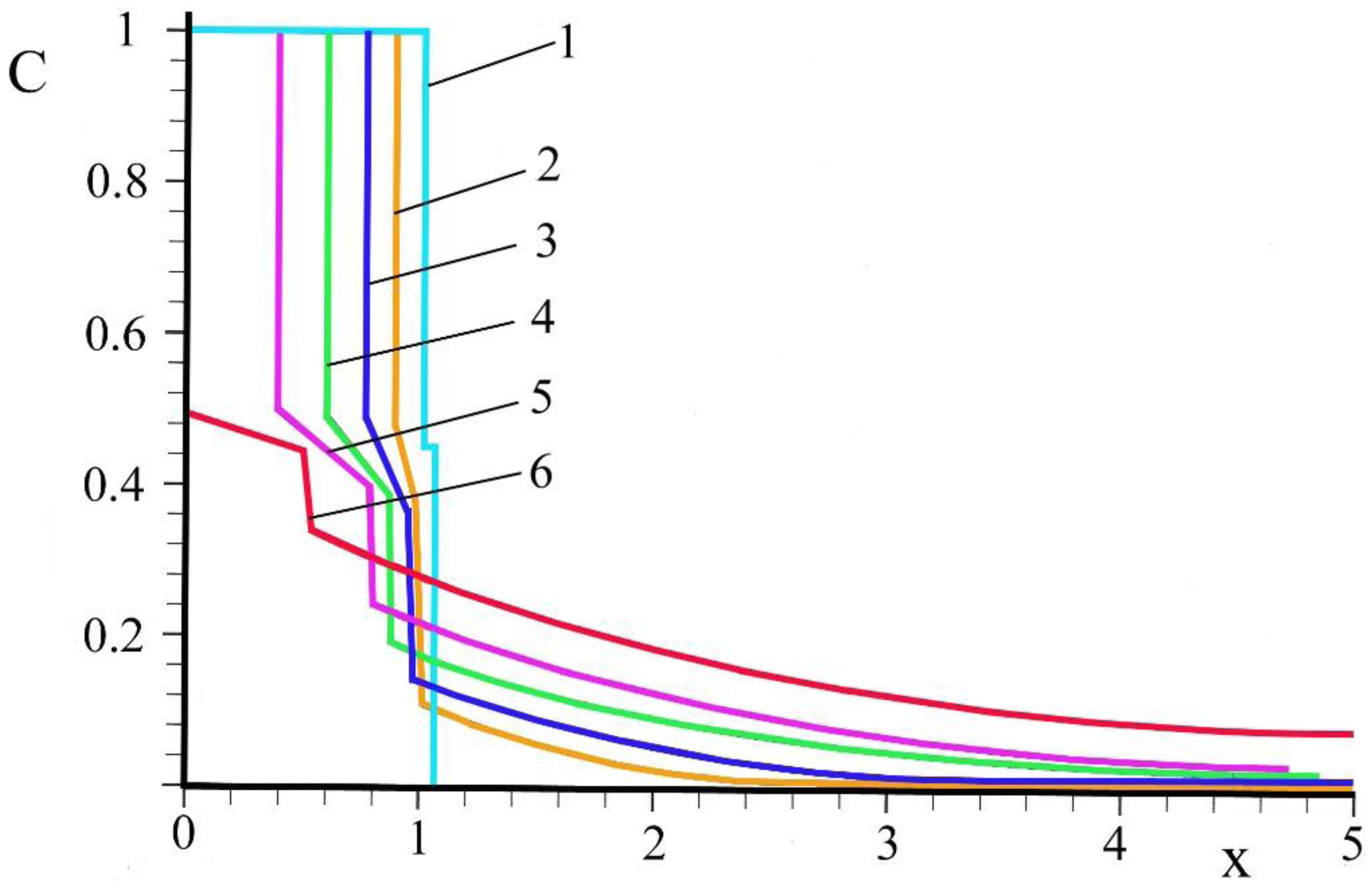
2.3. The Diffusion Model of Dissolution Refractory Inclusions in Metals under Concentrated Flows of Energy Action

Let us consider the dissolution of a high-melting element in liquid titanium, taking carbon as an example. A mathematical model and a method to solve the problem of carbon distribution in titanium carbide and in liquid titanium and carbon solution are considered below in terms of the state diagram and temperature changes caused by phase transitions and heat exchange with the ambient environment. The dependence of temperature of the surrounding cell environment with respect to time is the key feature of this model. This problem can be reduced to a non-autonomous singular differential second-degree equation, but it is difficult to analyze it in terms of quality [21,26,47]. Therefore, a numerical method is selected to investigate some definite models with particular parameters.

In the model below a cell is considered, which contains a r₀ size carbon particle, placed into liquid titanium with a definite volume of R₀ size. On the С-Ti interface a chemical reaction takes place, as the result of which titanium carbide generates and heat releases. A wave of titanium carbide generation with the coordinate r₁(t) starts spreading towards carbon. Carbon, which is diffusing through the layer TiC, reacts with titanium, as the result, carbide is generated, therefore, front r₂(t) is moving. Carbon also dissolves in liquid titanium. Hence, a three-layer structure is generated in the cell: hard carbon—0 < r < r₁, titanium carbide—r₁ < r < r₂, carbon solution in liquid titanium—r₂ < r < R₀. If temperature is assumed to be constant, mathematical statement of the diffusive problem contains the level of diffusion, edge, and initial conditions. Let us consider T_e < T < T_m in more detail: here T_e, T_m are the temperatures of eutectic titanium-titanium carbide and titanium carbide-graphite.

Equations of diffusion (sphere—n = 2, cylinder—n = 1, flat plate—n = 0) are as follows:

$$\begin{gathered} \frac{\partial c_{\mathrm{V}}(r,t)}{\partial t}=\frac{1}{r^n}\frac{\partial }{\partial r}\left(D_1{r}^n\frac{\partial c_{\mathrm{V}}(r,t)}{\partial r}\right),r_1(t)<r<r_2(t) \\ \frac{\partial c_{\mathrm{V}}(r,t)}{\partial t}=\frac{1}{r^n}\frac{\partial }{\partial r}\left(D_2{r}^n\frac{\partial c_{\mathrm{V}}(r,t)}{\partial r}\right),r_2(t)<r<R_0 \end{gathered}$$

(32)

Edge conditions on the extremities of the interval:

$$\begin{array}{l}{c}_{\mathrm{V}}(r_1(t)+0,t)=c_{\mathrm{V}1},c_{\mathrm{V}}(r_2(t)-0,t)=c_{\mathrm{V}2}\\ c_{\mathrm{V}}(r_2(t)+0,t)=c_{\mathrm{V}3},{\frac{\partial c_{\mathrm{V}}(r,t)}{\partial r}|}_{R_0}=0\end{array}$$

(33)

Conditions to determine the coordinates of boundaries:

$$\begin{gathered} (1-c_{\mathrm{V}1})\frac{d{r}_1}{dt}=D_1{\frac{\partial c_{\mathrm{V}}(r,t)}{\partial r}|}_{r_1+0},r_1(0)=r_0 \\ (c_{\mathrm{V}2}-c_{\mathrm{V}3})\frac{d{r}_2}{dt}=-D_1{\frac{\partial c_{\mathrm{V}}(r,t)}{\partial r}|}_{r_2-0}+D_2{\frac{\partial c_{\mathrm{V}}(r,t)}{\partial r}|}_{r_2+0},r_2(0)=r_0 \end{gathered}$$

(34)

Initial conditions:

$$c_{\mathrm{V}}(r,0)=\{\begin{array}{c}1,0<r<r_0\\ 0,r_0<r<R_0\end{array}$$

(35)

Here $c_{\mathrm{V}}=V_{\mathrm{C}}/(V_{\mathrm{C}}+V_{\mathrm{Ti}})$is the inclusion volume fraction of carbon in phases, which depends on the spatial values r and time t; V_J are the volumes of corresponding pure components (J = C, Ti). Figure 3 shows the graph of atomic fraction $c=N_{\mathrm{C}}/(N_{\mathrm{C}}+N_{\mathrm{Ti}})$ dependent on the coordinate. Atomic fracture can be used to determine the chemical formulae of phases. However, equations of diffusion are written for inclusion volume fractions or mass fractions, mole or atomic concentrations, which are proportional to them. Atomic-inclusion volume fraction conversion and vice versa are described in Equation (36):

$$c_{\mathrm{V}}=\frac{1}{\left(\frac{1}{c}-1\right)\frac{{\mathsf{\rho }}_{\mathrm{C}}}{{\mathsf{\rho }}_{\mathrm{Ti}}}\frac{{\mathsf{\mu }}_{\mathrm{Ti}}}{{\mathsf{\mu }}_{\mathrm{C}}}+1},c=\frac{1}{\left(\frac{1}{c_{\mathrm{V}}}-1\right)\frac{{\mathsf{\rho }}_{\mathrm{Ti}}}{{\mathsf{\rho }}_{\mathrm{C}}}\frac{{\mathsf{\mu }}_{\mathrm{C}}}{{\mathsf{\mu }}_{\mathrm{Ti}}}+1}$$

(36)

To calculate the temperature in the cell we use the heat-balance equation:

$$\begin{gathered} {С}_0{\mathsf{\nu }}_0\frac{dT}{dt}=Q_1\frac{d{\mathsf{\nu }}_1}{dt}+Q_2\frac{d{\mathsf{\nu }}_2}{dt}-a(T-T_{\mathrm{a}}(t)) \\ {\mathsf{\nu }}_1(t)={\displaystyle \underset{r_1}{\overset{r_2}{\int }}{c}_{\mathrm{V}}(r,t)r^n}dr,{\mathsf{\nu }}_2(t)={\displaystyle \underset{r_2}{\overset{R_0}{\int }}{c}_{\mathrm{V}}(r,t)r^n}dr \\ {\mathsf{\nu }}_0=\frac{1}{n+1}{R_0}^{n+1}\left(c_{\mathrm{V}0}+\frac{{\mathsf{\rho }}_{\mathrm{Ti}}}{{\mathsf{\mu }}_{\mathrm{Ti}}}\frac{{\mathsf{\mu }}_{\mathrm{C}}}{{\mathsf{\rho }}_{\mathrm{C}}}(1-c_{\mathrm{V}0})\right) \end{gathered}$$

(37)

Here (i = 1, 2). C₀ is the mean molar capacity of the cell, ${\mathsf{\nu }}_1,{\mathsf{\nu }}_2,{\mathsf{\nu }}_0$ are values, proportional to the moles of carbon in titanium carbide and in solution, as well as to the total mole concentration at the initial instant of time, the proportionality factor is similar. Q_i is the molar heat of titanium carbide generation and carbon dissolution in liquid titanium, respectively; and c_V is the bulk concentration of carbon in titanium carbide or in solution, $c_{\mathrm{V}0}={(r_0/R_0)}^{n+1}$ is the initial bulk concentration of carbon in the system, ρ_J and μ_J are the density and molar mass of the component J (J = C, Ti), a is the coefficient of heat exchange, T is the temperature of the cell, and T_a is the ambient temperature. We admit that the dependence of ambient temperature on time is pre-set.

The stated mathematical problem Equations (32)–(37) are solved numerically by the method of scalar marching. Time is assumed to be discrete at the moments $t_n=k\mathsf{\tau }$, τ is the time interval of discretization, and k is the time step number. Let us consider the values $c_{\mathrm{V}}^k,r_1^k,r_2^k,T^k$ to be known for the k time step, we calculate the values for k + 1 time step. An initial-boundary value problem is numerically solved with edge conditions and coefficients of diffusion, taken from k time step.

Calculations were done for a one-dimensional case (n = 0, flat plate), half-thickness of the cell to be calculated R₀, the initial half-thickness of graphite impurity r₀. Parameters of calculations are as follows: D₁₀ = 45.4 × 10⁻⁴ m²/s, E₁ = 447.5 × 10³ J/mol, D₂₀ = 38.5 × 10⁻⁴ m²/s, E₂ = 22.4 × 10³ J/mol, $c_{2\mathrm{e}}=0.31$,$T_{\mathrm{e}}=1926 \mathrm{K}$, $T_{\mathrm{m}}=3346 \mathrm{K}$, and Q₁ = 231.7 kJ/mol, δ = 0.1 [48].

Ambient temperature was decreasing according to the linear law$T_{\mathrm{a}}=T_{00}-\mathsf{\beta }t$. Here β is the rate of cooling. Parameters T₀₀, α, and β were varied. Initial temperature was selected equal to T₀₀. This approach helped to analyze whether carbon could dissolve in titanium, to determine its dissolution time according to initial temperature and the rate of cooling.

Figure 3 and Figure 4 show the results of calculations when the rate of cooling is equal to zero and there is no heat exchange. Values for r₀ were selected equal to either 10 µm or 10 nm. This was done to compare the time of carbon dissolution under conditions of various scales of cells.

The thickness of titanium carbide layer increases first, then it gets smaller (Figure 3). The time of dissolution is getting reduced as the initial temperature grows (Figure 4a,b). Here, if initial thickness of graphite layer reduces from 10 µm to 10 nm, time of dissolution decreases 10⁶ times. The time of graphite dissolution is on the order of microseconds; this conforms to the experiments on the electron-beam treatment of the surface after electro-explosive doping [10].

Therefore, the submitted model and calculations made on its ground, made it possible to demonstrate that micrometer-order carbon particles dissolve for about 10 s. This time goes far beyond the time of impact on material by concentrated flow of energy. If the dimensions of the particles are of nanometer-order ones, the time of dissolution gets equal to 10 μs in order of magnitude. In this case carbon particle can be dissolved as long as it is treated by electron-beam. We can say that the process of combined treatment requires for carbon-graphite fibers, micro-fibrille diameter of them is about tens of nanometers.

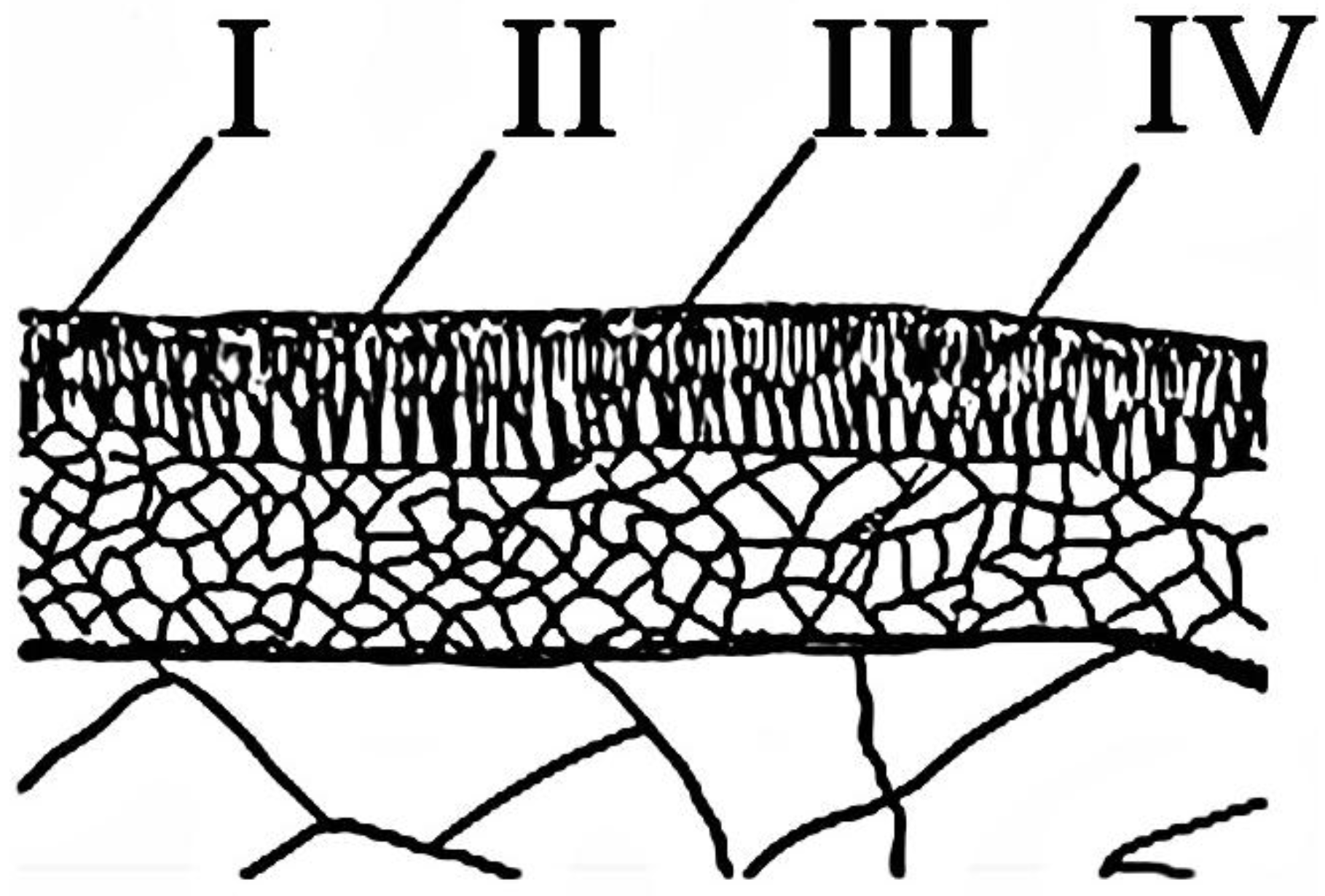
3. Modeling of Subsurface Nanostructure Formation

The research into the impact of the electric conductor, explosive-produced, heterogeneous plasma flows on the structure and properties of materials has demonstrated that a multi-layer gradient structure forms at a distance from the treated surface (Figure 5). The first ~1-µm thick nano-structural layer (I) reacts with plasma of incident flow [49]. The dimensions of vertically-located cells in the second layer (II) with the structure of cellular-type crystallization are much larger than those located horizontally. The third layer (III) has approximately equal longitudinal and crosscut dimensions of the grain. The forth inner nano-structural layer (IV) is ~1 µm thick. These experimental facts, two nano-structural layers in particular, have become the issue of theoretical investigations. The external nano-layer is possible to account for the significant heat removal and, as a consequence, for the high rate of cooling. However, specific conditions are necessary in order to obtain such significant rates of cooling, which is hardly ever possible. The internal nano-layer could not be modeled in the thermal model. Moreover, this layer was considered an artifact. Nevertheless, in products hardened quickly from the melt on a rapidly-moving disk (hardening by spinning) there are four structural zones, described in [50]. The zone located near to the surface to be hardened, or the zone of freezing, has a fine, disperse structure. It is thought to be generated as the result of multiple-crystal nucleation. The second zone is one of columnar crystal—highly extended grains. A dendrite or dendrite-cellular structure is formed in the third zone. The fourth zone is one of equiaxed randomly-oriented nano-grains. The situation here is much aike that one described above—an internal nano-layer arises under the action of heterogeneous plasma. Furthermore, nano-dimensional structures, which form under significant plastic deformations, arise, if two materials are sheared. Nanostructures were detected in shear bands, when detailed microscopic research was carried out [29]. The aforementioned experimental data emphasizes nanostructures to appear often in shear flows.

In [51] one explains why the first nano-structural layer arises involving the mechanism of Kelvin-Helmholtz instability [30] in the nano-dimensional range of wavelengths in conditions of tangentiall- flowing plasma and a layer of molten metal. If two media are moving relative to each other, waves appear (like ripples on water’s surface when it is windy). A dispersion evolution is obtained in linear approximation of the evolving boundary surface which is, as a rule, a transcendental algebraic equation attributing increments to the wavelength. This depends on a number of parameters; hence, analytical parameterization can rarely be accomplished. Therefore, a dispersion equation is solved numerically to obtain the dependence of the decrement on the wavelength for definite values of parameters.

The maximums in this dependence are obtained at particular wavelengths λ_max under conditions of positive increments. Hence, ~λ_max-dimensioned waves, and vortices generated by them, are developed, and waves of other lengths, other scales, respectively, cannot be formed. This approach is a conventional one for investigations into instabilities. The idea of using this mechanism to explain the generation of the second internal nano-layer (zone IV) was offered and elaborated in [30]. In this work the following dispersion relation is obtained in the approximation of viscous and viscous-potential fluid in terms of Navier-Stokes and Euler equations.

To derive a dispersion equation we deal with a double-layer incompressible liquid (Figure 6), like in [30]. The underlayer is assumed to be fixed and viscous. The upper layer is modeled as a perfect liquid moving at speed u₀ parallel to the underlayer. For each layer Navier-Stocks and Euler linearized equations are written:

$$\begin{array}{l}\frac{\partial U_1}{\partial t}=-\frac{1}{{\mathsf{\rho }}_1}\frac{\partial P_1}{\partial x}+{\mathsf{\nu }}_1\left(\frac{{\partial }^2{U}_1}{\partial x^2}+\frac{{\partial }^2{U}_1}{\partial y^2}\right)\\ \frac{\partial V_1}{\partial t}=-\frac{1}{{\mathsf{\rho }}_1}\frac{\partial P_1}{\partial y}+{\mathsf{\nu }}_1\left(\frac{{\partial }^2{V}_1}{\partial x^2}+\frac{{\partial }^2{V}_1}{\partial y^2}\right),\frac{\partial U_1}{\partial x}+\frac{\partial V_1}{\partial y}=0\end{array}$$

(38)

For the upper layer:

$$\frac{\partial U_2}{\partial t}+u_0\frac{\partial U_2}{\partial x}=-\frac{1}{{\mathsf{\rho }}_2}\frac{\partial P_2}{\partial x},\frac{\partial V_2}{\partial t}+u_0\frac{\partial V_2}{\partial x}=-\frac{1}{{\mathsf{\rho }}_2}\frac{\partial P_2}{\partial y},\frac{\partial U_2}{\partial x}+\frac{\partial V_2}{\partial y}=0$$

(39)

Kinematic and dynamic conditions on the boundary of layers:

$$\begin{array}{l}y=H:V_2=0,y=-h:U_1=0,V_1=0\\ y=0:\frac{\partial \mathsf{\eta }}{\partial t}+u_0\frac{\partial \mathsf{\eta }}{\partial x}=V_2,\frac{\partial \mathsf{\eta }}{\partial t}=V_1\\ -P_1+P_2+2{\mathsf{\rho }}_1{\mathsf{\nu }}_1\frac{\partial V_1}{\partial y}=\mathsf{\sigma }\frac{{\partial }^2\mathsf{\eta }}{\partial x^2}+g({\mathsf{\rho }}_2-{\mathsf{\rho }}_1)\mathsf{\eta }\end{array}$$

(40)

We note that index 1 is for the underlayer, whereas index 2 is for the upper one. Equations (38) and (39) are solved the following way:

$$\begin{array}{l}{U}_1(x,y,t)=u_1(y)\exp (\mathsf{\omega }t-ikx),U_2(x,y,t)=u_2(y)\exp (\mathsf{\omega }t-ikx)\\ V_1(x,y,t)=v_1(y)\exp (\mathsf{\omega }t-ikx),V_2(x,y,t)=v_2(y)\exp (\mathsf{\omega }t-ikx)\\ P_1(x,y,t)=p_1(y)\exp (\mathsf{\omega }t-ikx),P_2(x,y,t)=p_2(y)\exp (\mathsf{\omega }t-ikx)\\ \mathsf{\eta }={\mathsf{\eta }}_0\exp (\mathsf{\omega }t-ikx)\end{array}$$

(41)

Substituting Equation (41) into Equations (38)–(40) and carrying out further transformations we obtain a dispersion equation:

$$\begin{array}{l}G(z,d)+\mathsf{\mu }{\mathsf{\Omega }}_1^2\mathrm{cth}(kH)+W=0\\ G(z,d)=\frac{\left(\left(z^4-1\right)\left(z-\mathrm{th}\left(zd\right)\mathrm{th}\left(d\right)\right)\right)}{\left(\mathrm{th}\left(zd\right)-z\mathrm{th}\left(d\right)\right)}{\mathsf{\nu }}^2+\frac{2z\left(1-z^2\right){\mathsf{\nu }}^2-2z\left(z^2+3\right){\mathsf{\nu }\mathsf{\nu }}_1}{\mathrm{sh}\left(zd\right)\mathrm{ch}\left(d\right)-z\mathrm{sh}\left(d\right)\mathrm{ch}\left(zd\right)}\\ +\frac{\left(2z\left(z^2+3\right)-2\left(1+3z^2\right)\mathrm{th}\left(d\right)\mathrm{th}\left(zd\right)\right)}{\left(\mathrm{th}\left(zd\right)-z\mathrm{th}\left(d\right)\right)}{\mathsf{\nu }\mathsf{\nu }}_1\end{array}$$

(42)

where ${\mathsf{\Omega }}_1=\frac{\mathsf{\Omega }}{k^2}=\mathsf{\nu }(z^2-1)i-\frac{u_0}{k}$, $\mathsf{\mu }=\frac{{\mathsf{\rho }}_2}{{\mathsf{\rho }}_1}$, $W=\frac{A}{{\mathsf{\rho }}_1{k}^3}=\frac{g({\mathsf{\rho }}_2-{\mathsf{\rho }}_1)-{\mathsf{\sigma }}_0{k}^2}{{\mathsf{\rho }}_1{k}^3}$, and ν₁ is the viscosity on the boundary of layers. We consider cases when the underlayer is viscous or viscous-potential liquid. In the first case ${\mathsf{\nu }}_1=\mathsf{\nu }$, so Equation (42) is written as follows:

$$\begin{array}{l}{\mathsf{\nu }}^2{G}_1(z,d)+\mathsf{\mu }{\mathsf{\Omega }}_1^2\coth (kH)+W=0\\ G_1(z,d)=\frac{-4z(z^2+1)}{\sinh (zd)\cosh (d)-z\sinh (d)\cosh (zd)}+\\ \frac{z(z^4+6z^2+5)-(z^4+6z^2+1)\tanh (d)\tanh (zd)}{\tanh (zd)-z\tanh (d)}\end{array}$$

(43)

For viscous-potential liquid ν = 0 and ν₁ ≠ 0, so Equation (42) is written:

$$\begin{array}{l}{G}_2(z,d)+\mathsf{\mu }{\left(\frac{\mathsf{\nu }-k{u}_0}{k^2}\right)}^2\coth (kH)+W=0\\ G_2(z,d)=\frac{2i\mathsf{\omega }}{\tanh (d)}{\mathsf{\nu }}_1+\frac{{\mathsf{\omega }}^2}{k^4\tanh (d)}\end{array}$$

(44)

The analysis of this relation has demonstrated that increment dependencies on the wavelength for viscous and viscous-potential liquids are nearly the same in the wide range of parameters (Figure 7). Therefore, a less complicated dispersion equation of viscous-potential liquid can be applied to analysis in terms of the quality of Kelvin-Helmholtz instability of a perfect and viscous liquid boundary. Numerical computations of increment dependencies on the wavelength at definite values of parameters, which are like those of internal nano-layer formations under the action of heterogeneous plasma flows on ferrum, have revealed that two maximums in the increment-wavelength dependence—in the micro- and nano-range—are possible, if a moving layer is thin (ρ₁ = ρ₂ = 6.3 × 10³ kg/m³, ν = 6 × 10⁻⁷ m²/s, σ₀ = 1.2 N/m [52], h = 10⁻⁶ m, H = 10⁻⁶ m, u₀ = 30 m/s). This conforms to the development of two-mode instability.

The microwave mode corresponds with the interaction of perfect liquid layers. The nano-wave mode is formed due to viscosity. In general, the offered interpretation has the following results. In H = h = 1-µm thick layers, if the rates exceed 40 m/s, λ = 1-µm long waves arise; for these values of layer thickness and wavelength the wave can be considered as a moving H_c ≈ 10-nm thick boundary layer, where a nano-wave mode is developing; the wavelength is λ_c = 100 nm.

4. Conclusions

• A thermal mathematical model, which considers vaporization from the surface of the material, has been presented. The dependence of penetration depth vs. energy surface density is obtained. Its linear character has been shown. When comparing penetration depths determined computationally with the experimental data their satisfactory fit has been determined. The period of vaporization has been determined without solving the gas-dynamic problem.
• The mechanism of bipolar thermo-elastic wave generation has been revealed on the basis of being solved analytically, not on the basis of the uncoupled thermo-elasticity problem. The matter of it is that tension and compression in the thermo-elastic wave are caused by an increase and a subsequent drop of temperature on the edge.
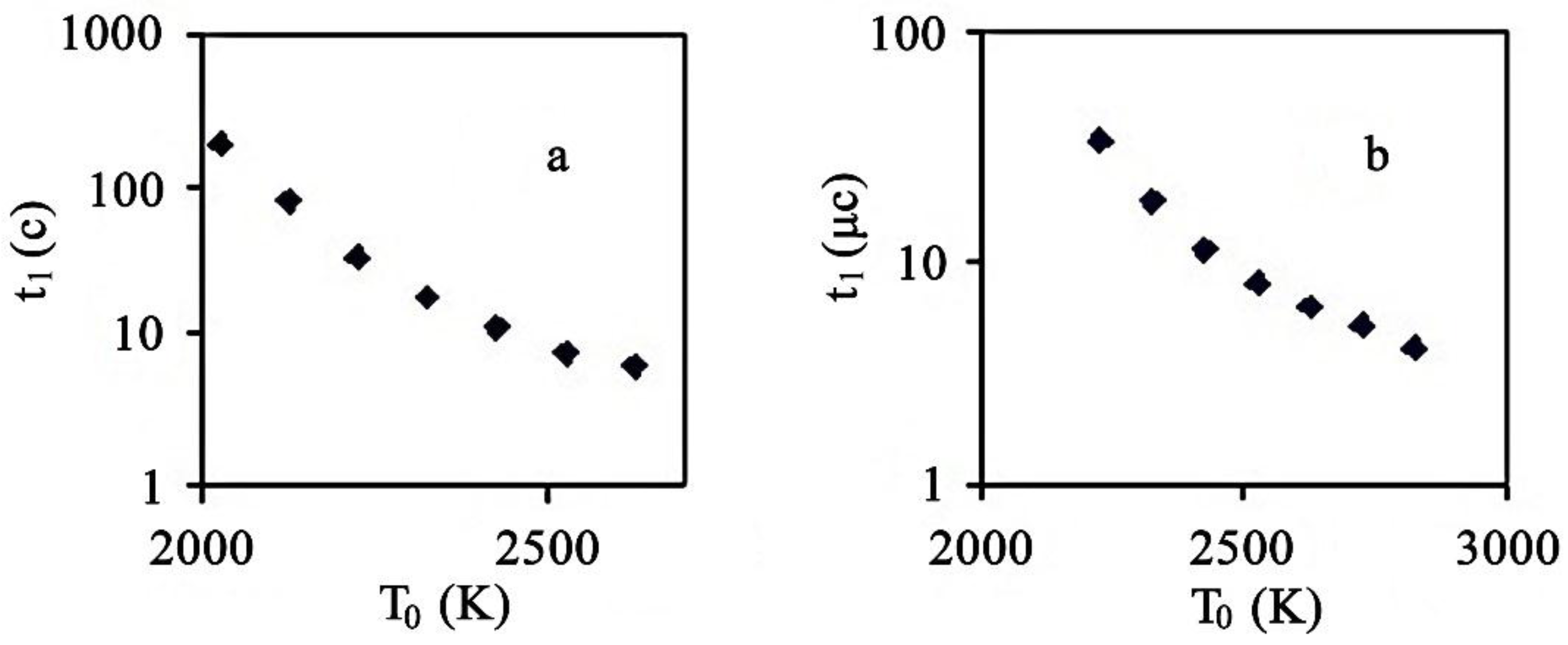
• A model of the dissolution of carbon particles in titanium has been analyzed under the action of electron beams. It has been stated that micrometer-dimensional carbon particles get dissolved for about 10 s. This time significantly exceeds the time of concentrated energy flow impact on the material. If particles are nanometer-dimensional ones, the time of dissolution is 10 μs in order of magnitude. In this case carbon particles get dissolved as long as they are impacted by electron beams.
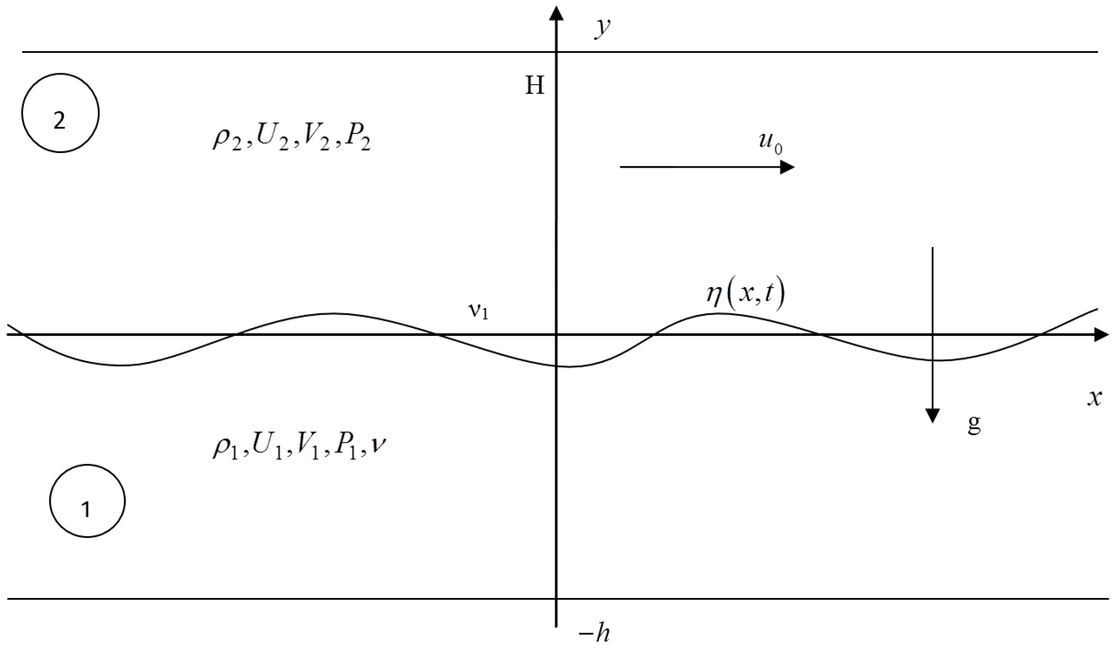
• Formation of internal nano-structural layers has been analyzed under the action of heterogeneous plasma flows. Instability increment dependence on the wavelength with two maximums—in nano- and micro- ranges—have been developed.

References

1. Ilyuschenko, A.P.; Shevtsov, A.I.; Astashynski, V.M.; Kuzmitski, A.M.; Gromyko, G.F.; Chumakov, A.N.; Bosak, N.A.; Buikus, K.V. Friction and wear of powder coatings produced by using high-energy pulsed flows. High Temp. Mater. Process. 2015, 19, 141–152. [Google Scholar] [CrossRef]
2. Huang, Z.-T.; Suo, H.-B.; Yang, G.; Yang, F.; Dong, W. Effect of heat treatment on microstructure and property of TC18 titanium alloy prepared by electron beam rapid manufacturing. Trans. Mater. Heat Treat. 2015, 36, 50–54. [Google Scholar]
3. Da Silva, M.R.; Gargarella, P.; Gustmann, T.; Filho, W.J.B.; Kiminami, C.S.; Eckert, J.; Pauly, S.; Bolfarini, C. Laser surface remelting of a Cu-Al-Ni-Mn shape memory alloy. Mater. Sci. Eng. A 2016, 66, 161–167. [Google Scholar] [CrossRef]
4. Chen, X.; Wang, J.; Fang, Y.; Madigan, B.; Xu, G.; Zhou, J. Investigation of microstructures and residual stresses in laser peened Incoloy 800H weldments. Opt. Laser Technol. 2014, 57, 159–164. [Google Scholar] [CrossRef]
5. Hu, J.; Chai, L.; Xu, H.; Ma, C.; Deng, S. Microstructural modification of brush-plated nanocrystalline Cr by high current pulsed electron beam irradiation. J. Nano Res. 2016, 41, 87–95. [Google Scholar] [CrossRef]
6. Zhou, Z.; Chen, B.; Xiao, H.; Tu, J.; Chai, L.; Huang, W.; Hu, J. Microstructure and properties of CuFe10 alloys treated by high current pulsed electron beam. High Power Laser Part. Beams. 2015, 27, 024105. [Google Scholar] [CrossRef]
7. Devyatkov, V.N.; Koval, N.N.; Schanin, P.M.; Grigoryev, V.P.; Koval, T.V. Generation and propagation of high-current low-energy electron beams. Laser Part. Beams 2003, 21, 243–248. [Google Scholar] [CrossRef]
8. Sosnin, K.V.; Raykov, S.V.; Vaschuk, E.S.; Budovskikh, E.A.; Gromov, V.E.; Ivanov, Y.F. Morphology of the surface of technically pure titanium VT1-0 after electroexplosive carbonization with a weighed zirconium oxide powder sample and electron beam treatment. In Proceedings of the International Conference on Physical Mesomechanics of Multilevel Systems, Tomsk, Russia, 3–5 September 2014.
9. Sosnin, K.V.; Raikov, S.V.; Gromov, V.E.; Ivanov, Y.F.; Budovskikh, E.A.; Vashchuk, E.S. Formation of a microcomposite structure in the surface layer of yttrium-doped titanium. J. Surf. Investig. X-ray Synchrotron Neutron Tech. 2015, 9, 377–382. [Google Scholar] [CrossRef]
10. Ivanov, Yu.F.; Teresov, A.D.; Petrikova, E.A.; Raikov, S.V.; Goryushkin, V.F.; Budovskikh, E.A. Surface layer of commercially pure VT1-0 titanium after electric-explosion alloying and subsequent treatment by a high-intensity pulsed electron beam. Steel Transl. 2013, 43, 798–802. [Google Scholar] [CrossRef]
11. Markov, A.B.; Rotshtein, V.P. Calculation and experimental determination of hardening and tempering zones in quenched U7A steel irradiated with a pulsed electron beam. Nucl. Instrum. Methods Phys. Res. Sect. B 1997, 132, 79–86. [Google Scholar] [CrossRef]
12. Markov, A.B.; Ivanov, Yu.F.; Proskurovsky, D.I.; Rotshtein, V.P. Mechanisms for hardening of carbon steel with a nanosecond high-energy, high-current electron beam. Mater. Manuf. Process. 1999, 14, 205–216. [Google Scholar] [CrossRef]
13. Leyvi, A.Ya.; Talala, K.A.; Krasnikov, V.S.; Yalovets, A.P. Modification of the Constructional Materials with the Intensive Charged Particle Beams and Plasma Flows. Ser. Mech. Eng. Ind. 2016, 16, 28–55. (In Russian) [Google Scholar]
14. Mazhukin, V.I.; Mazhukin, A.V.; Lobok, M.G. Mathematical modeling of dynamics of fast phase transitions and overheated metastable states during nano- and femtosecond laser treatment of metal targets. Math. Model. Comput. Simul. 2010, 2, 396–405. [Google Scholar] [CrossRef]
15. Bleykher, G.A.; Krivobokov, V.P.; Yuryeva, A.V. Thermal Processes and Emission of Atoms from the Liquid Phase Target Surface of a Magnetron Sputtering System. Russ. Phys. J. 2015, 58, 431–437. [Google Scholar] [CrossRef]
16. Yalovets, A.P. Calculation of flows of a medium induced by high-power beams of charged particles. J. Appl. Mech. Tech. Phys. 1997, 38, 137–150. [Google Scholar] [CrossRef]
17. Khaimzon, B.B.; Sarychev, V.D.; Gromov, V.E. Temperature distribution produced by pulsed energy fluxes, with evaporation of the target. Steel Transl. 2013, 43, 55–58. [Google Scholar] [CrossRef]
18. Maier, A.E.; Yalovets, A.P. Mechanical stresses in an irradiated target with a disturbed surface. Tech. Phys. 2006, 51, 459–465. [Google Scholar] [CrossRef]
19. Chumakov, Yu.A.; Knyazeva, A.G. Interrelated processes of heat mass transfer and stress evolution in a disk with an inclusion under the action of high density energy flow. Phys. Mesomech. 2013, 16, 85–91. [Google Scholar]
20. Sarychev, V.D.; Voloshina, M.S.; Gromov, V.E. Mathematical model of generation of the thermoplastic waves under action of concentrated energy fluxes at the materials. Basic Probl. Mater. Sci. 2011, 8, 71–76. (In Russian) [Google Scholar]
21. Lyubov, B.Ya. Diffusion Processes in Nonhomogeneous Solid State; Nauka: Moscow, Russia, 1981. (In Russian) [Google Scholar]
22. Bukrina, N.V.; Knyazeva, A.G. Numerical solution algorithm for non-isothermal diffusion problems in surface treatment processes. Phys. Mesomech. 2006, 9, 55–62. (In Russian) [Google Scholar]
23. Knyazeva, A.G.; Krukova, O.N.; Bukrina, O.V.; Sorokova, S.N. Simulation issues of surface treatment and coating materials using high energy sources. Izv. TPU 2010, 317, 93–101. (In Russian) [Google Scholar]
24. Merzhanov, A.G.; Averson, A.E. The present state of the thermal ignition theory: An invited review. Combust. Flame 1971, 16, 89–124. [Google Scholar] [CrossRef]
25. Nekrasov, E.A.; Smolyakov, V.K.; Maksimov, Yu.M. Adiabatic heating in the titanium-carbon system. Combust. Explos. Shock Waves 1981, 17, 305–311. [Google Scholar] [CrossRef]
26. Khina, B.B. Combustion Synthesis of Advanced Materials; Nova Science Publishers Inc.: New York, NY, USA, 2010. [Google Scholar]
27. Aleksandrov, V.V.; Korchagin, M.A. Mechanism and macrokinetics of reactions accompanying the combustion of SHS systems. Combust. Explos. Shock Waves 1987, 23, 557–564. [Google Scholar] [CrossRef]
28. Sarychev, V.D.; Khaimzon, B.B.; Gromov, V.E. Mathematical model of dissolution of particles of carbon in the titan at influence of the concentrated streams of energy. Titan 2012, 1, 4–8. (In Russian) [Google Scholar]
29. Sarychev, V.D.; Mochalov, S.P.; Budovskikh, E.A.; Vashchuk, E.S.; Gromov, V.E. Formation of convective structures in metals and alloys under the action of pulsed multiphase plasma jets. Steel Transl. 2010, 40, 531–536. [Google Scholar] [CrossRef]
30. Granovskii, A.Yu.; Sarychev, V.D.; Gromov, V.E. Model of formation of inner nanolayers in shear flows of material. Tech. Phys. 2013, 58, 1544–1547. [Google Scholar] [CrossRef]
31. Inogamov, N.A.; Zhakhovsky, V.V.; Khokhlov, V.A.; Petrov, Y.V.; Migdal, K.P. Solitary nanostructures produced by ultrashort laser pulse. Nanoscale Res. Lett. 2016, 11, 177. [Google Scholar] [CrossRef] [PubMed]
32. Suh, K.Y.; Jeong, H.E.; Kim, D.-H.; Singh, R.A.; Yoon, E.-S. Capillarity-assisted fabrication of nanostructures using a less permeable mold for nanotribological applications. J. Appl. Phys. 2006, 100, 034303. [Google Scholar] [CrossRef]
33. Prokoshev, V.G.; Parfionov, S.D.; Obgadze, T.A. Mathematical modelling of the temperature fields induced under the laser processing material. In Proceedings of the International conference on laser assisted net shape engineering LANE 2001, Erlangen, Germany, 28–31 March 2001; pp. 185–190.
34. Galkin, A.F.; Abramov, D.V.; Savina, L.D.; Fedotova, O.Yu.; Prokoshev, V.G.; Arakelian, S.M. Laser-induced hydrodynamics waves on the surface of melt. In Proceedings of the Laser-induced hydrodynamics waves on the surface of melt, Vladimir/Suzdal, Russia, 21 September 2000; Volume 4429, pp. 101–104.
35. Lee, P.D.; Quested, P.N.; McLean, M. Modelling of Marangoni effects in electron beam melting. Philos. Trans. R. Soc. A Math. Phys. Eng. Sci. 1998, 356, 1027–1043. [Google Scholar] [CrossRef]
36. Lukashov, E.A.; Radkevich, E.V.; Yakovlev, N.N. Structurization of the instability zone and crystallization. J. Math. Sci. 2011, 179, 491–514. [Google Scholar] [CrossRef]
37. Kuznetsov, V.P.; Smolin, I.Y.; Dmitriev, A.I.; Tarasov, S.Y.; Gorgots, V.G. Toward control of subsurface strain accumulation in nanostructuring burnishing on thermostrengthened steel. Surf. Coat. Technol. 2016, 285, 171–178. [Google Scholar] [CrossRef]
38. Sarychev, V.D.; Nevskii, S.A.; Konovalov, S.V.; Komissarova, I.A.; Cheremushkina, E.V. Thermocapillary model of formation of surface nanostructure in metals at electron beam treatment. IOP Conf. Ser. Mater. Sci. Eng. 2015, 91, 012028. [Google Scholar] [CrossRef]
39. Sarychev, V.D.; Nevskii, S.A.; Sarycheva, E.V.; Konovalov, S.V.; Gromov, V.E. Viscous Flow Analysis of the Kelvin–Helmholtz Instability for Short Waves. In Proceedings of the International Conference on Advanced Materials with Hierarchical Structure for New Technologies and Reliable Structures 2016, Tomsk, Russia, 19–23 September 2016; Volume 1783.
40. Samarskii, A.A.; Babishchevich, P.N. Vychislitel’naya Teploperedacha (Computational Heat Transmission); Editorial URSS: Moscow, Russia, 2003. [Google Scholar]
41. Cheynet, B.; Dubois, J.-D.; Milesi, M. Données thermodynamiques des éléments chimiques. Tech. Ing. Traité Mater. Metall. 1993, M64-1–M64-22. [Google Scholar]
42. Missenard, A. Conductivite Thermique des Solides, Liquides, Gaz et Leurs Melanges; Editions Eyrolles: Paris, France, 1965. [Google Scholar]
43. Iesan, D.; Antonio, S. Thermoelastic Deformations; Springer: Berlin, Germany, 1996. [Google Scholar]
44. Awrejcewicz, J.; Krysko, V.A. Nonclassical Thermoelastic Problems in Nonlinear Dynamics of Shells; Springer: Berlin, Germany, 2003. [Google Scholar]
45. Three-Dimensional Problems of the Mathematical Theory of Elasticity and Thermoelasticity; Kupradze, V.D. (Ed.) Elsevier: Amsterdam, The Netherlands, 1976.
46. Proskurovsky, D.I.; Rotshtein, V.P.; Ozur, G.E.; Ivanov, Y.F.; Markov, A.B. Physical foundations for surface treatment of materials with low energy, high current electron beams. Surf. Coat. Technol. 2000, 125, 49–56. [Google Scholar] [CrossRef]
47. Paul, T.; Vuorinen, V.; Divinski, S.V.; Laurila, T. Thermodynamics, Diffusion and the Kirkendall Effect in Solids; Springer: Berlin, Gemany, 2014. [Google Scholar]
48. Mehrer, H. Diffusion in Solids; Springer: Berlin, Germany, 2007. [Google Scholar]
49. Bagautdinov, A.Ya.; Tsvirkun, O.A.; Budovskikh, E.A.; Ivanov, Yu.F.; Gromov, V.E. Gradient state of the surface layers of iron and nickel after electro-explosive alloying. Metallurgist 2007, 51, 151–158. [Google Scholar] [CrossRef]
50. Glezer, A.M.; Permyakova, I.E. Melt-Quenched Nanocrystals; CRC Press: Boca Raton, FL, USA, 2013. [Google Scholar]
51. Bazylev, B.; Janeschitz, G.; Landman, I.; Loarte, A.; Klimov, N.S.; Podkovyrovd, V.L.; Safronov, V.M. Experimental and theoretical investigation of droplet emission from tungsten melt layer. Fusion Eng. Des. 2009, 84, 441–445. [Google Scholar] [CrossRef]
52. Forsythe, W.E. Smithsonian Physical Tables; Knovel: Norwich, NY, USA, 2003. [Google Scholar]
Figure 1. The temperature dependence of coordinates on time t1 = 31 μs. Here are xV(t) and xL(t). The calculations are carried out for ES = 60 J/sm2, t0 = 100 μs.
Metals 07 00004 g001
Figure 2. The dependence of stress on the coordinates: in the instants of non-dimensional time: (а) 0.21; and (b) 0.41.
Metals 07 00004 g002
Figure 3. The dependencies of atomic fraction of carbon (C) according to the value x = r/r0. 1: 0, 2: 1.2, 3: 2.5, 4: 3.8, 5: 5.0, 6: 6.136 (μs) (initial temperature 2626 К, r0 = 10 nm).
Metals 07 00004 g003
Figure 4. Time dependence of graphite dissolution on initial temperature of the cell: (а) r0 = 10 µm; (b) r0 = 10 nm.
Metals 07 00004 g004
Figure 5. The arrangement of four structural zones.
Metals 07 00004 g005
Figure 6. Computation scheme.
Metals 07 00004 g006
Figure 7. Increment α dependencies on the wave length λ for various H and σ0 = 1.2 N/m. Full line—viscous model, dotted line—viscous-potential. (1) H = 6 nm; (2) H = 10 nm; (3) H = 20 nm; and (4) H = 30 nm.
Metals 07 00004 g007