Abstract
Gas metal arc welding (GMAW) is a joining process that is controlled by several inputs or welding parameters. However, speed, current and voltage are the parameters that are most frequently used in setting this process. Cord area, yield stress, tensile strength, residual stresses, hardness and roughness are considered to be outputs or welded joints parameters. They are widely used when the design requirements are based on the cost, manufacturing speed, strength and surface finish. This paper seeks to determine the relationship between the welding parameters and the welded joint parameters of speed, current and voltage in butt joints (X-groove) of EN 235JR by the response surface method (RSM). The optimal joints when considering the design requirements of cost, manufacturing speed, strength and surface finish were achieved by using the multi-response surface (MRS). The optimal welding parameters reached when considering the design requirements of cost were 140.593 amps, 8.192 mm/s and 29.999 volts, respectively, whereas the design requirements of manufacturing speed were 149.88 amps, 9.261 mm/s and 29.999 volts. Finally, the welding parameters for the design requirements of joint strength and surface finish were 149.086 amps, 7.139 mm/s and 28.541 volts and 150.372 amps, 8.561 mm/s and 29.877 volts, respectively.
1. Introduction
Gas metal arc welding (GMAW) is a metal joining process that is commonly used in many industrial sectors. A wide range of materials can be joined by GMAW, although stainless steel and low carbon steel are the materials that typically are welded by this technique. Due to the intense concentration of heat in a reduced area, the areas that are near the weld cord experience severe thermal cycles, which generate residual stresses and changes in mechanical properties. Several inputs or process parameters can be controlled directly by the welding machine or robot (speed, voltage, current, wire feed rate, flow rate of shielding gas and flux proportion of the mixture). Alternatively, they can be controlled by the boundary conditions (nozzle-to-plate distance, electrode orientation, plate thickness and wire diameter). However, speed, voltage and current are the most frequently-used parameters in the design process of welded joints that are manufactured by GMAW [1,2]. In this regard, yield stress and tensile strength are the outputs or welded joint parameters that are used widely to determine the accumulated plastic strain, which is closely related to the amount of energy absorbed before the welded joint fails [3]. Residual stresses are produced mainly by non-uniform heat distributions and plastic deformations and can provide information on changes in microstructural phases [4]. Tensile residual stresses are induced by shrinkage of the molten region, and compression residual stresses are induced by the effect of phase transformations [5]. The maximum values of residual stresses usually appear in the heat-affected zone (HAZ) on the toe of the weld cord and should be reduced as much as possible [6]. Variations in the residual stresses among the base metal, weld cord and HAZ can cause an increase in corrosion, as well as the formation of an irregular surface of the welded joints [7]. A surface roughness (Ra) of 3–4 µm can be achieved on high-quality weld cords, but values of 7–8 µm are more likely on industry standard welds cords [8]. Micro-hardness and hardness are usually used to quantify the strength of each constituent in the weld joint by determining the average hardness of each phase [9]. Some researchers [10,11] have investigated the relationship between hardness and tensile strength and used it to assess the strength of the welded joint. High values of hardness in the welded zone may be attributed to a fine grain size [12,13]. Lower values of hardness in the HAZ may be related to grain growth and a ferrite phase in this region [14,15]. In this sense, it is necessary for the difference between the hardness levels of parent material, weld cord and HAZ to be as low as possible so that the strength of the weld is as homogeneous as possible [16]. Moreover, the power consumed during the manufacture of welded joints affects greatly the yield, tensile strength, residual stresses and hardness. Similarly, the inputs or process parameters have a considerable influence on the weld area and power that is consumed, which can provide an idea of the amount of material that is provided to the welded joint. For example, the power that is consumed, the speed and the amount of filled material that is provided for the weld cord also should be considered, since they markedly affect the total manufacturing cost of welded products. The most desirable welded joint is the one that has the lowest possible values of residual stresses, surface roughness (Ra), hardness and manufacturing cost, but with its yield stress, tensile strength and speed maximized. The process of achieving the optimal welded joint solely on the basis of trial-and-error when the design requirements of cost, strength and surface finish are considered is a difficult task that should result in an unacceptable cost. In this context, some researchers have used the response surface methodology (RSM) in order to reduce the number of experiments that are necessary to obtain the optimal combination of inputs or process parameters. RSM is a statistical method that is used widely to model and optimize processes. It uses the input variables of the process and their responses or outputs to identify the combined effect of the input variables and obtain the best response [17]. RSM attempts to replace the implicit functions of the original design optimization problem with an approximation model that is traditionally a polynomial function (regression models) and, therefore, less expensive to evaluate. When there is more than one output, several response surfaces should be optimized using MRS. In this paper, a group of regression models that are based on the RSM was used to determine the relationship between the welding process parameters (inputs) and the welded joints parameters (outputs). Then, while considering design requirements based on manufacturing cost, manufacturing speed, strength and surface finish, the optimal welded joints were achieved by the MRS with the desirability functions. The weld cord area is the welded joint parameter that is used when the design requirements are based on the cost, whereas yield stress, tensile strength, residual stresses and hardness are the parameters used when the design requirements are based on the welded joint strength. Finally, roughness (Ra) is the parameter that is used when the design requirements are based on the surface finish. This paper concentrates on a study of the butt joint with complete penetration (X-groove) of EN 235JR low carbon steel for a range of speeds, currents and voltages for inputs or process parameters of 120–180 amps, 3–10 mm/s and 20–30 volts. The remaining inputs or process parameters (flow rate of the shielding gas, orientation of the electrode and the distance between the nozzle and plate) were assumed to be constants with values of 20.0 L/min, 80° and 4.0 mm, respectively.
2. Modelling Using the RSM
The RSM is a method that attempts to determine the relationships between the independent variables (input variables) and one or more response variables (output variables). The method was introduced by Box and Wilson in 1951 [18] to use the data that are obtained by experiments to obtain a model or an optimal response. Originally, RSM was developed to model experimental responses. However, it has been used recently in combination with other techniques to optimize products and industrial processes [19,20]. Basically, RSM is a group of statistical techniques that utilizes a regression model that is based on a low-degree polynomial function (Equation (1)).
where Y is an experimental response, (x1, x2, x3, …, xk) are the vectors of inputs, e is an error and f is a function that consists of cross-products of the terms that form the polynomial. The quadratic model (second-order) is one of the most widely-used polynomial functions and is expressed in Equation (2):
where the first summation is the linear part, the second is the quadratic part and the third is the product of the pairs of all variables. The values of the coefficients b0, bi, bii and bij are calculated by using regression analysis. Nevertheless, these functions sometimes do not give good results for complex problems with many nonlinearities and a high number of inputs. This is because they are continuous functions that are defined by polynomials and cannot be adjusted when the data are sparse. The p-value (or Prob. > F) is defined as the probability of obtaining a result that is equal to or greater than what was actually observed, assuming that the model is accurate. It can be computed by the analysis of variance (ANOVA). If the Prob. > F of the model and no term in the model exceeds the level of significance (say α = 0.05), the model may be considered to be adequate within a confidence interval of (1 − α). Some researchers have used ANOVA with the aim of analysing the influence of the inputs or process parameters on the outputs of the process [21,22]. When a problem has more than one output, it is called MRS and implicates conflict between outputs because an optimal configuration for one output may differ greatly from the optimal for another output. Harrington [23] presented a compromise between outputs. It consisted of desirability functions for each output, Equations (3) and (4), and an overall desirability that is defined as the geometric mean of the desirability D for each output (Equation (5)).
where A and B are the limit values and s is an exponent that determines how important it is to reach the target value; X is the input vector; and fr is the model that is used for prediction. A second higher degree polynomial should be used to optimize one or several responses [24]. The desirability approach involves transforming each estimated response into a unitless utility that is bounded by 0 < dr < 1, where a higher value of dr indicates that the response value is more desirable. The optimization part of the R package v.1.6, [25] searches for a combination of importance factors (or weights from 1–3) that simultaneously satisfy the optimization criteria of each of the responses and inputs.
3. Welded Joint Parameters that Were Studied Using RSM
Several researchers have used the RSM to obtain the optimal combination of inputs or process parameters in welded joints. However, most of these works are based on the modelling and optimization of a relatively low number of output and input parameters. Thus, for example, hardness is commonly employed to investigate the grain size distribution of the welded joint and is characterized by means of a micro-hardness test. The test is carried out by a micro Vickers-hardness testing machine [26] and is used to obtain a surface hardness map with the values of hardness at different points across the weld joint [27,28]. High values of hardness in the welded zone may be attributed to fine grain size [12,13], whereas lower values of hardness in the HAZ may be related to grain growth [14,15,29]. In this regard, different levels of hardness that are obtained at the different parts of the weld joint could affect the overall behaviour of a weld joint. This can cause small cracks and material discontinuities, as well as the appearance of residual stresses. Some researchers have studied the micro-hardness test results of welded joints to create a hardness map of different points across the weld joint. Ghazanfari et al. [9] developed a comparative micro-hardness study of AISI 4130 welded joints to obtain hardness maps of the weld cord, base metal and heat-affected zone (HAZ) for a tungsten inert gas welding process (TIG). Other authors, such as Samardžić et al. [16], have studied the influence of welding parameters on hardness at different points across the weld joint in the submerged arc welding process (SAW). In this case, the study sought to reduce the level of hardness of different areas of the welded joint when the input parameters varied. One of the first works to be undertaken was a statistical study by Darwish et al. [30]. In this case, the influence of the input parameters on hardness and tensile strength of the weld joint was modelling using a linear regression model. Jindal et al. [31] modelled a hardness and weld cord area according to the welding parameters of SAW using the mathematical models that were obtained from the RSM. In this case, the hardness at the centre of a weld bead of the welded joint (fusion zone) was determined.
Yield stress and tensile strength are widely used in the characterization of the structural integrity and strength of welded joints. Obtaining these parameters is always undertaken by means of standard tests [32,33] that reveal, for different areas of the welded joint (parent material, weld bean and heat-affected zone (HAZ)), the plastic strain that accumulates until total failure occurs [3]. Knowing the strength of the welded joint is very important, since it predicts the performance of the joint in service. Thus, for example, if failure of the weld joint occurs on the weld cord, the joint is deficient. However, if failure of the parent material occurs, the joint is oversized. In this sense, several authors have investigated the method of modelling and optimizing the strength of the welded joint. For example, Dwivedi et al. [34] studied the influence of the process parameters (rated power of the microwave oven, welding time and temperature) on microwave welding. In this case and using RSM, the tensile strength of the welded joints was modelled and optimized. This study demonstrated that the strength of the welded joints decreases with increasing rated power, whereas the tensile strength of a welded joint increases as the welding time and the welding temperature increase.
Mechanical properties also are strongly influenced by residual stresses, which are one of the most important parameters considered during the manufacture of welded joints. The magnitude of residual stresses that are obtained should be in the vicinity of the HAZ, as measured in standard tests [35]. Several authors have studied the modelling and optimizing of residual stresses for various welding parameter inputs or process parameters. For example, Olabi et al. [36] determined the relationship between laser welding parameters and the magnitude of the residual stress at different locations by using RSM for laser butt-welding of AISI 304 plates joints. In a similar fashion, Olabi et al. [37] studied the minimization of residual stress in the heat-affected zones of AISI 304 plates that were welded with LBW (laser beam welding). This optimization was conducted by several designs of experiment (DOE) techniques, the Taguchi method and RSM. The process input parameters that were considered for both cases were: laser power, welding speed and focal point position. Furthermore, the incremental hole-drilling method was employed to measure the magnitude and distribution of the maximum residual stress in both studies [38].
Surface roughness can directly influence the quality of the surface, the tensile and yield stress and the fatigue strength of the welded joint. Surface roughness is determined by the mean roughness [39]. It is often used as a standard to measure the surface finish and quality of welded joints [40]. A weld joint with mean values of 3–4 µm of roughness should be considered to be a high-quality weld, whereas values of 7–8 µm are more likely encountered on industry-standard welds [8]. Furthermore, surface roughness can be affected by each of the parameters that control the welding processes. In this regard, Tzeng [41] studied as the input welding parameters speed, pulse energy, average peak power density and pulse duration to determine how they affected the mean roughness values of a welded joint that is manufactured by pulsed laser welding. The study showed that, as the mean laser power increased, the roughness of the weld bead was less pronounced when an acceptable welding speed was applied. Moreover, if the average laser power is reduced to a certain limit, the roughness values increase rapidly. Furthermore, Alam et al. [42] studied the influence of roughness on the tensile strength and fatigue strength at welded joints that were manufactured by laser hybrid welding. Although the fatigue strength is often dominated by the toe radius of the welded joint, high roughness values cause high stresses to appear in the ripples of the weld cords. These values of high stress on the weld cord ripples somehow affect the fatigue and tensile strength of the welded joint.
The input parameters of the welding process have a considerable influence on the weld bead geometry and weld bead area. The weld bead area can provide an idea of the amounts of material that are provided to the welded joint and consumed by the welding process. Basically, all weld bead geometries are characterized by their penetration, width, reinforcement height, width-to-penetration ratio and percentage dilution. There have been many studies during recent decades of how various input parameters of different welding processes influence weld bead geometry. For example, Gunaraj and Murugan [43] used the RSM to develop mathematical models for use in relating the input process parameters in weld beads in SAW of pipes (open-circuit voltage, wire feed rate, welding speed and nozzle-to-plate distance) to the outputs or welded joint parameters (penetration, reinforcement, width and percentage dilution of the weld bead). They demonstrated that all outputs decrease with increasing welding speed, whereas an increase in the wire feed rate produces an increase in all outputs, except width. Benyounis et al. [44] applied RSM to determine the effect of the input process parameters in the laser welding process (laser power, welding speed and focal point position) in order to determine the heat input, penetration, bead width and width of HAZ outputs. They discovered that the laser power has a positive effect on all of the outputs or welded joint parameters. Based on this study, Benyounis et al. [45] optimized the previous welding process by utilizing MRS based on a desirability approach. More recently, Wang et al. [46] studied the mathematical relationship between input process parameters in the laser welding process (laser power, joining speed and stand-off-distance) and the strength and width of the weld joint using RSM. A central composite second-order rotational design (CCRD) was used, and the optimum-joining parameters were achieved. Singh et al. [47] used the MRS to predict the critical dimension of weld-bead geometry and shape relationships with the effect of polarity in submerged arc welding (SAW). In this case, bead width, penetration, reinforcement and percentage dilution of the welded joint were modelled when the input process parameters wire feed rate, open circuit voltage, travel speed and contact tip-to-work distance.
4. Experimental Setup and Results Obtained
All welded joints were manufactured automatically with an ABB 1500 IRB robot incorporated in an ESAB 180 welding machine (Figure 1a). During the GMAW process, all specimens were supported on a refractory flat surface to which both plates of EN 235JR low carbon steel were clamped. Thus, the unique forces that produced the angular distortion of the welded parts were only gravity and the force of thermal shrinkage. The cooling of the welded joints was accomplished in air at a room temperature of 18 °C. The weld cord was deposited sequentially on both sides of the plates to be welded (first on one side and then on the other side) to create a butt joint with complete penetration (X-groove). Figure 1b shows a schematic of how the welding process was developed for all specimens. The wire that was used for all specimens was an ER70S-6 with a diameter of 1.2 mm and a chemical composition and mechanical behaviour very similar to those of the base metal. The flow rate of the shielding gas and the distance between the nozzle and plate were 20.0 L/min and 4.0 mm, respectively, with an orientation of the electrode of 80°. The dimensions of the plates that were used to manufacture all welded joints were 60 × 80 × 6 mm, and the length of the weld cord was 60 mm. The gas mixture was 80% argon (Ar) and 20% carbon dioxide (CO2) (see Figure 1c). Each of the specimens was machined in order to obtain sufficient samples for the different welded joint characterization tests (see Figure 1d).
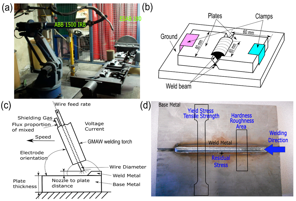
Figure 1.
(a) ABB 1500 IRB robot with the ESAB 180 welding machine used to manufacture all welded joints with gas metal arc welding (GMAW). (b) The welding process employed in the manufacture of the butt joint with complete penetration (X-groove). (c) Common welding parameters used in GMAW and considered in this case. (d) Butt joint with complete penetration (X-groove) manufactured: details of the specimens to be machined for the different welded joint characterization tests.
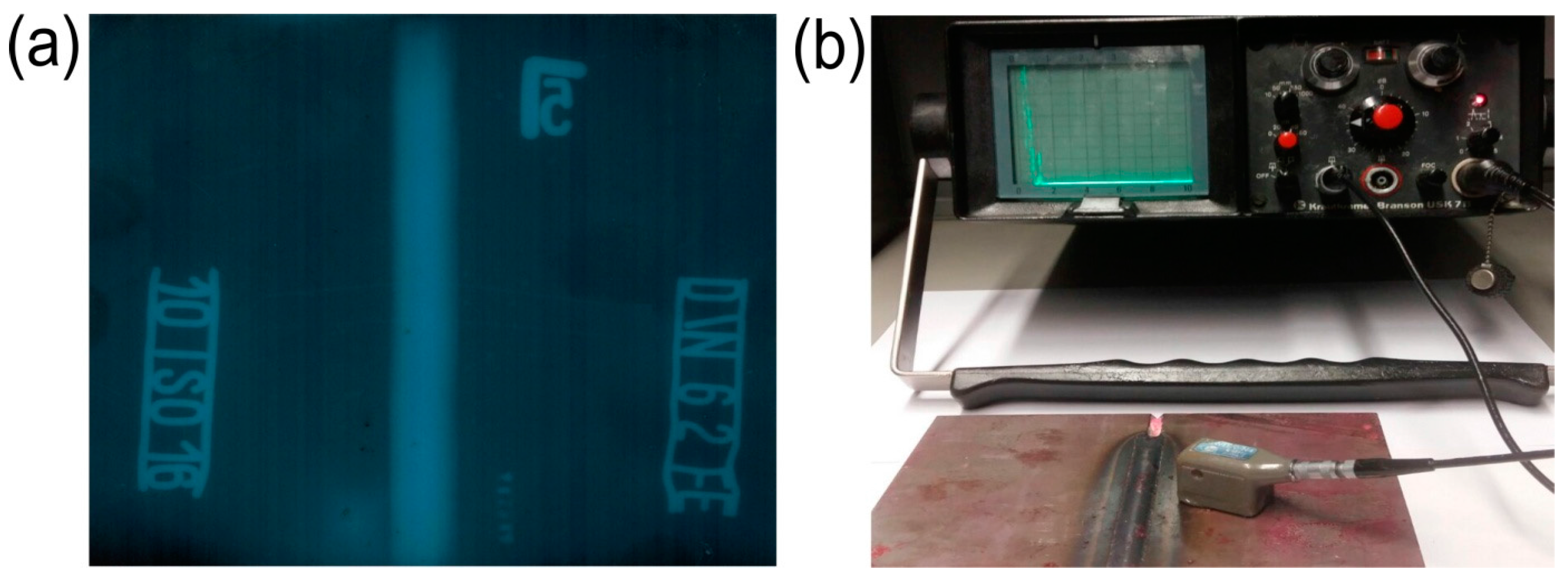
Prior to conducting the different tests for characterization of the welded joint, X-ray radiographic analysis and ultrasonic testing were undertaken according to ISO 17636 [48] and ISO 11666 [49], respectively, to detect possible defects and imperfections in the welded joints to be studied. These types of analysis are considered to be non-destructive testing and allow testing of the specimens studied to continue by other methods of analysis. The tests were conducted to identify welded joints to reject that might cause any alteration in the outputs or welded joints parameters that would be obtained and were undertaken with a Balteau X-ray radiographic analysis and Krautkramer USK7B ultrasonic analysis with MWB80-4 angle beam transducer equipment. Figure 2a shows the results of a radiographic analysis of a welded specimen on which no defects or imperfections were detected. Similarly, Figure 2b shows the procedure followed for an ultrasonic analysis.
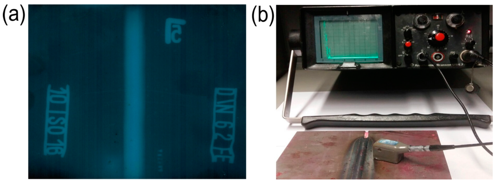
Figure 2.
(a) X-ray radiograph that shows a weld bead that was analysed. (b) Analysis using ultrasonic testing.
Once all specimens were checked by the nondestructive tests just mentioned and no defect or imperfections were detected, they were subjected to the following standard tests to characterize the welded joints.
4.1. Residual Stresses
It is known that different welding sequences applied to the same specimens can produce different residual strains and stresses on them [50]. In this case, all specimens were manufactured with the same welding sequence (same weld cord length and direction of welding) and were fixed to the ground in the same points (see Figure 1d). In the centre of the weld joint and on the left side of the weld cord in the direction of advance of the welding robot (as close as possible to the foot of the weld bead), the incremental hole-drilling non-destructive technique was used [38] to obtain the maximum residual stress. This technique is considered to be a stress-relaxing method that analyses the stress-relaxation that is produced in a metal part when the material is removed. This test was first so that the residual stresses were not altered by relaxation of the material that was machined for the final test that is required in this work. The procedure that was described in measurement group TN-503 [51] was followed. A strain gauge rosette type CEA-06-062UM-120, which allows the residual stresses close to the weld bead to be measured, was used to ensure that they were the maximum. Figure 3a shows the milling guide machine (Model RS-200, Vishay Measurements Group, Raleigh, NC, USA) with an ultra-high speed air turbine that includes a carbide cutter to drill a hole in the centre of the strain gauge rosette. Figure 3b shows the glued strain gauge rosette that contains a centre hole to relax the material close to the weld cord and obtain the residual stresses.
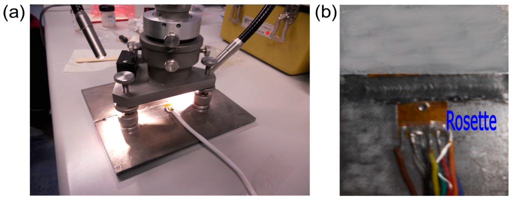
Figure 3.
(a) RS-200 milling guide machine. (b) Detail of the strain gauge rosette type CEA-06-062UM-120.
4.2. Hardness
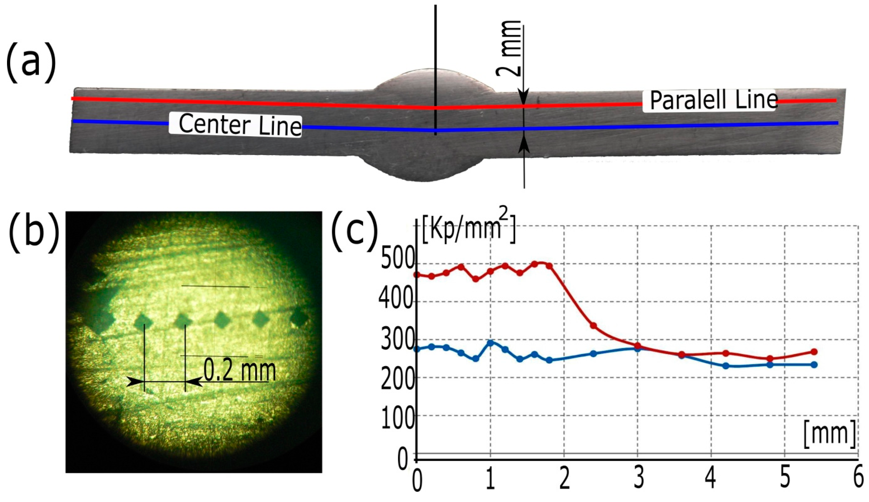
A Shimadzu micro Vickers-hardness type HMV-2 testing machine was used to obtain the difference between the average values of hardness obtained in the weld cord and the average values of hardness HV obtained in the centre line of the base metal according to ASTM E92 [26]. In this case, the value of the applied force was 1 kPa (or 9.81 N), and the holding time was 15 seconds (HV1). Before proceeding with the measurement of hardness, all welded joints were cut into pieces, ground and then treated with picric acid on the faces of the cuts in accordance with ASTM E407 [52], so that different areas of the joint would be visible (weld bead, HAZ and base metal). The value of hardness HV for the weld cord of all specimens was measured at different points in a straight line that was 2 mm from, and parallel to, the centre line of the weld joint. The distance between hardness HV measurements points was 0.2 mm. (Figure 4b). Figure 4c shows the variations of the hardness in the parallel straight line that is located 2 mm from the centre line of the weld joint in red and the centre line of the weld joint in blue. Figure 4c also shows that points on the weld bead have a much greater hardness than points on the base metal.

Figure 4.
(a) Lines in which the hardness values in both the weld and the base metal were measured. (b) Micrograph that shows the hardness HV values obtained every 0.2 mm. (c) Varying hardness values obtained in both lines (centre line and parallel line).
4.3. Yield Stress and Tensile Strength
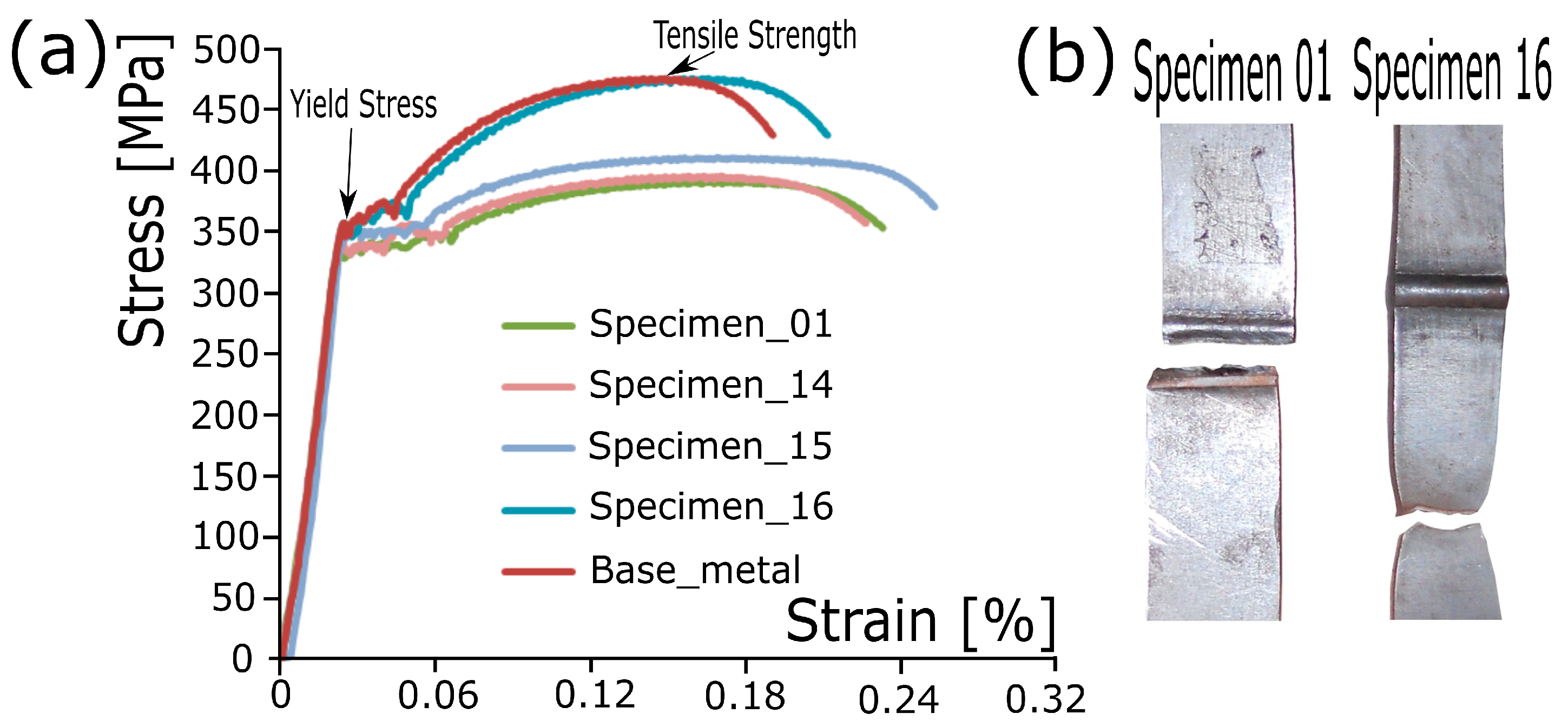
The specimens with which to obtain the values of yield stress and tensile strength were prepared according to the ASTM E8M-04 Standard Test Method and the ISO 5178 Standard Test Method, respectively [32,33], and were tested in a MAH-3000 Servosis universal testing machine. Figure 5a shows the yield stress and tensile strength that were obtained for some of the welded specimens, as well as for the base metal. Furthermore, the figure shows that the stress-strain curve for the base metal has a very similar behaviour to that of Specimen 16. This is mainly because Specimen 16 has a rigid weld cord, and welded joint failure occurs in the base metal, which is the element of the welded joint that suffers the most localized plastic deformation. Furthermore, Figure 5b shows some of the specimens after they were tested. This last figure shows that failure of the welded joint has occurred in the base metal (Specimen 01), whereas failure of the welded joint occurred in other specimens tested in the weld bead itself (Specimen 16). The failure of the welded joint in the base metal suggests that the weld cord was oversized, whereas the failure of the welded joint in the weld cord suggests that its dimensions were inappropriate.

Figure 5.
(a) Yield stress and tensile strength according to the ISO 5178 Standard Test Method. (b) Specimens after they were tested according to ISO 5178.
4.4. Surface Roughness
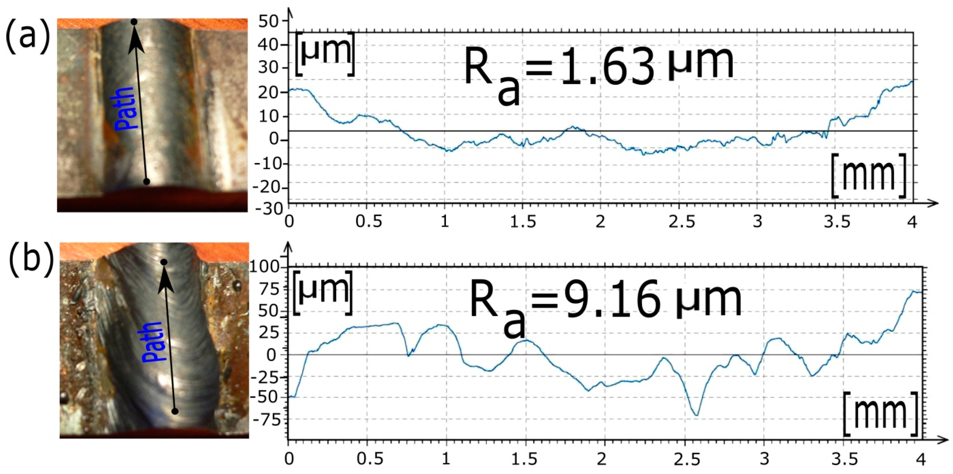
The roughness of the welded joints was measured longitudinally at the face of each bead. The roughness measurement was conducted according to the ISO 4287 standard [53] using a portable Surtronic 25 Taylor Hobson surface roughness tester profilometer. Figure 6 shows the roughness value obtained on the face of two different weld beads. The actual weld bead from which the roughness values were obtained (Ra) appears on the left side of each figure, as well as the path that the portable roughness tester probe followed to determine the roughness (right side). The face of the weld bead shown in Figure 6b has higher values of waves than those that appear in Figure 6a, which generate higher values of roughness. The profile of the roughness shown in Figure 6a has a lower roughness value (Ra = 1.63 μm) than the value that appears in Figure 6b (Ra = 9.16 μm).

Figure 6.
Roughness profile obtained and paths that the portable roughness tester probes followed to determine the roughness. (a) Low values of roughness obtained and (b) high values of roughness obtained.
4.5. Weld Cord Area Surface Roughness
To obtain the weld cord area, the joint was cut into pieces and ground. Then, the faces of the cuts were treated with picric acid according to ASTM E407 [52]. Once the specimens had been treated, they were examined under a microscope using 40× magnification. The images obtained by the microscope were digitalized. Subsequently, software was used to determine the surface of each weld bead. Figure 7 shows the areas obtained for two weld beads that were created by the GMAW process with different input process parameters of current, voltage and speed. Figure 7a (Specimen 09) shows an area of the weld cord that is much greater than that of the weld cord that appears in Figure 7b (Specimen 09). The amount of filler material in Specimen 09 suggests that the filler material used to create the welded joint is excessive for the thickness of the welded plates studied.
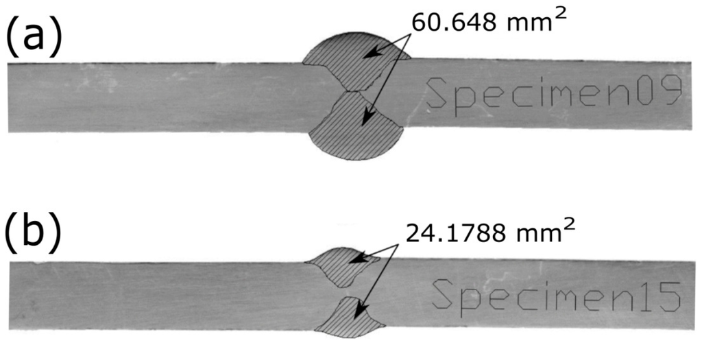
Figure 7.
Weld cord areas at different GMAW input process parameters of current, voltage and speed.
5. Design of Experiments
RSM needs to establish a DoE [54] in order to obtain accurate models with the least amount of data to support the initial hypotheses. Several methods have been proposed to develop DoE. However, they all require the construction of a design matrix (inputs) to measure the outputs or responses of the experiments. In this case, a Box–Behnken design (BBD) [55] of three factor and three levels was used to develop the experiment. The input process parameters that were used to develop the DoE were speed (S), current (C) and voltage (V). The outputs were area of the weld cord (A), surface roughness (Ra), hardness (H), yield stress (YS), tensile strength (TS) and the maximum residual stress (RS). The range in which the different levels of current, speed and voltage were adjusted was based on the experience of the laboratory personnel, as well as on the manufacturing of a group of preliminary welded samples in order to ensure that the welded specimens had no defects and imperfections. Thus, for example, Figure 8 shows some preliminary tests in which the specimens that were manufactured present defects and imperfections. Figure 8a shows a weld bead in which the flow rate of the shielding gas and the orientation of the electrode are incorrect (in this case, 10.0 L/min and 65°, respectively, when the correct values are 20.0 L/min and 80°, respectively (see Section 4)). In this figure, the pores in the weld cord are visible. They have been caused by a poor melting of the filler material cord. Furthermore, Figure 8b shows a weld joint that was manufactured with the following input parameters: a current of 260 amp, a voltage of 30 volts and a speed of 3 mm/s. In this case, the heat supplied during the welding process was excessive and caused the metal base, which had a thickness of 6 mm, to melt.
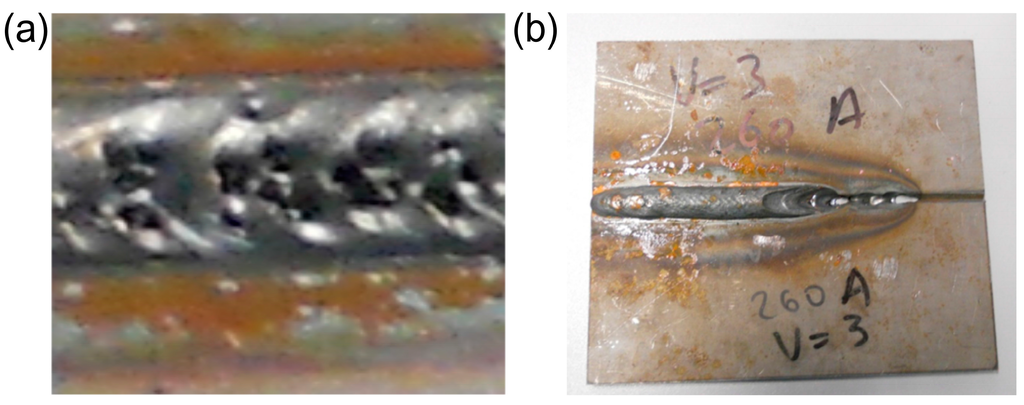
Figure 8.
(a) Pores in the weld cord due to incorrect values of flow rate of the shielding gas and the orientation of the electrode. (b) Melting of the base metal due to excessive heat supplied to the welding process.
Once the input process parameters that could cause defects and/or imperfections were discarded on the basis of inspection of the preliminary welded samples and the experience of the laboratory personnel, the ranges for each of the input process parameters were established. Table 1 shows the input process parameters, the notation and the limits of each input parameter.

Table 1.
Independent variables and experimental design levels used with the Box–Behnken design (BBD) method.
According to the input parameters and levels shown in Table 1 and using the statistical open source software R (r-project) [56], 17 experiments were generated with their corresponding inputs (Table 2).
Table 2.
Design matrix and specimens obtained by BBD. A, area of the weld cord; H, hardness; YS, yield strength; TS, tensile strength; RS, residual stress.
6. Results and Discussion
6.1. Modelling the Area, Yield Stress, Tensile Strength, Roughness and Residual Stress Using RSM
Equations (6)–(11) were fitted by using the data that appear in Table 2 to obtain regression equations for all responses. The RMS “R” package [57] was used for this. Second-order polynomial models were built for each response, and several criteria (R2, p-value, MAE and RMSE) were used to select the most accurate model. These equations show the second degree polynomial functions that were obtained to model area (A), roughness (Ra), hardness (H), yield stress (YS), tensile strength (TS) and residual stresses (RS). These equations show how each of the outputs is obtained by a combination of second-order polynomials that are formed by a combination of input variables.
A = 70.108 − 11.955 × S − 0.0159 × C × S + 0.716 × S2 − 1.337 × V + 0.0142 × C × V
Ra = 30.084 − 0.284 × C + 0.001094 × C2 + 7.566 × S − 0.0285 × C × S + 0.1416 × S2 − 2.455 × V + 0.0054 × C × V − 0.201 × S × V + 0.059 × V2
H = 1524.363 − 7.828 × C − 29.685 × S + 0.159 × C × S + 1.448 × S2 − 46.377 × V + 0.261 × C × V
YS = −2156.353 +30.110 × C − 0.085 × C2 − 167.101 × S + 0.882 × C × S − 2.888 × S2 + 48.827 × V − 0.355 × C × V + 2.351 × S × V
TS = −2794.565 + 32.582 × C −0.0729 × C2 − 135.596 × S + 0.699 × C × S − 2.539 × S2 + 80.884 × V − 0.559 × C × V + 2.012 × S × V
RS = 907.235 − 27.519 × C + 0.103 × C2 + 0.214 × C × S + 3.620 × S2 + 86.219 × V − 0.202 × C × V − 2.382 × S × V − 0.622 × V2
Table 3, Table 4, Table 5, Table 6, Table 7 and Table 8 show the results of ANOVA for each of the final quadratic models. Most of the variables have a p-value that is less than 0.01. This indicates that the variables that were used on the reduced quadratic models are statistically significant. The multiple correlation coefficient (R2) was calculated as the measure of the amount of variation around the mean that was obtained by the regression model. The results showed that all values of R2 are close to one. This indicates that these models possess good predictive capacity.
Table 3.
ANOVA table for the “A” quadratic model.
Table 4.
ANOVA table for the “Ra” quadratic model.
Table 5.
ANOVA table for the “H” quadratic model.
Table 6.
ANOVA table for the “YS” quadratic model.
Table 7.
ANOVA table for the “TS” quadratic model.
Table 8.
ANOVA table for the “RS” quadratic model.
MAE and RMSE are calculated to determine the generalization capacity of the quadratic models that are obtained using the data that appear in Table 2 according to Equations (12) and (13).
In this case, YkExperiment are the responses that were obtained experimentally, and YkModel are those that were obtained from the quadratic models that were developed with RSM and m specimens. Table 9 shows the prediction errors, where the maximum error corresponds to YS (MAE equal to 6.826 and RMSE equal to 7.345), and the minimum error corresponds to RS (MAE equal to 2.993 and RMSE equal to 3.504).
Table 9.
Results of the predicted error criteria for area (A), roughness (Ra), hardness (H), yield stress (YS), tensile strength (TS) and residual stresses (RS).
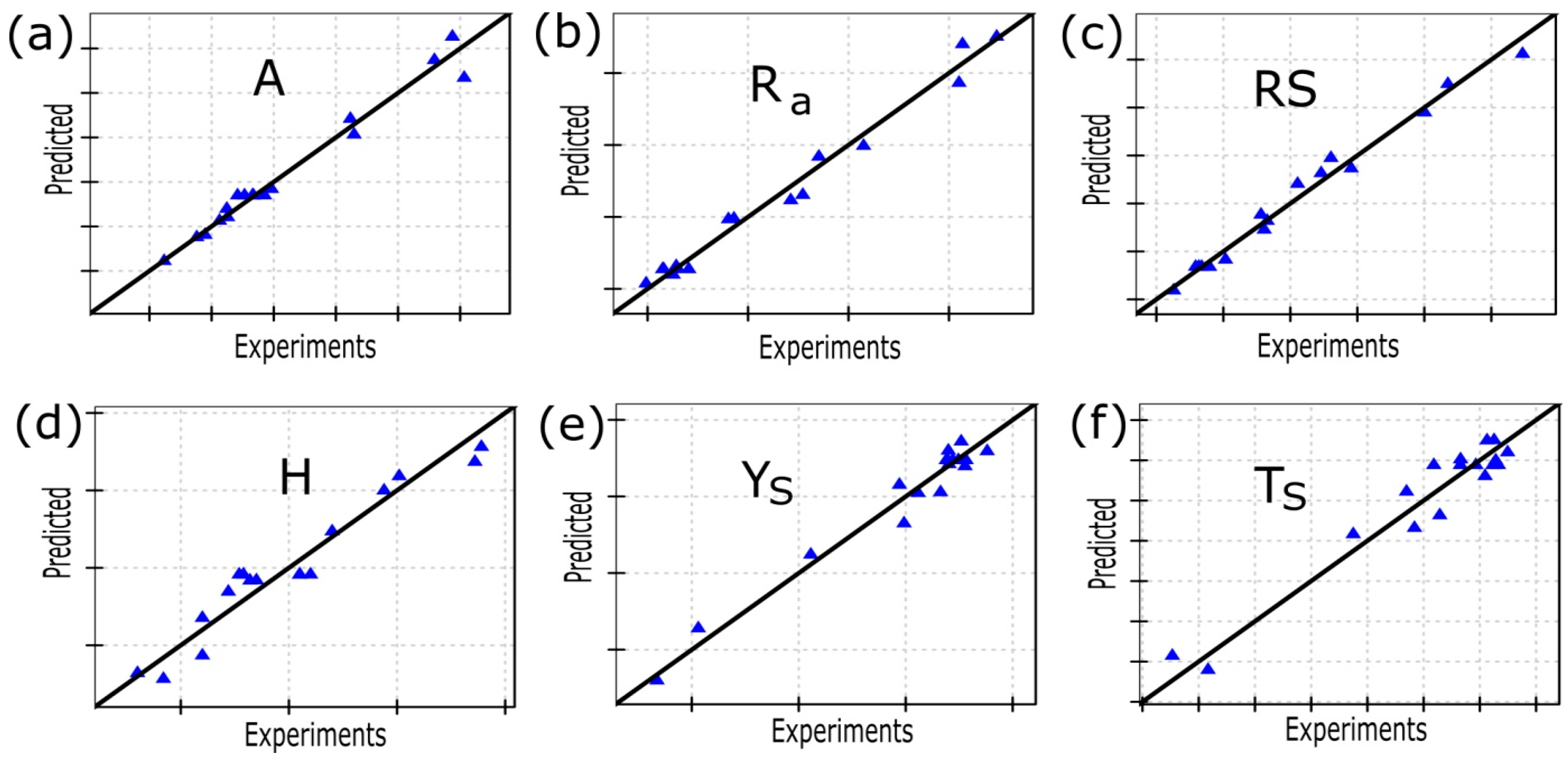
Figure 9 shows the relationship between the actual values that were obtained experimentally (Table 1) and the predicted (quadratic models) values of A (Figure 9a), Ra (Figure 9b), H (Figure 9c), TS (Figure 9d), YS (Figure 9e) and RS (Figure 9f). The figures show that these models are adequate for the prediction of these values because the residuals that were obtained are small and the correlations between actual and predicted values are high.
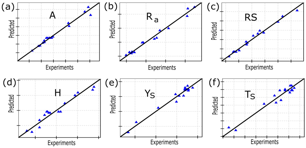
Figure 9.
Scatter diagram of: (a) area (A), (b) roughness (Ra), (c) residual stress (RS), (d) hardness (H), (e) yield stress (YS) and (f) tensile strength (TS).
6.2. Multi-Response Optimization
Table 10, Table 11, Table 12, Table 13 and Table 14 show the combination of process parameters and welded joint parameters that were studied in searching the design process of welded joints through desirability functions using the RMS “R” package [25], while considering several design requirements. The first column of all tables shows the inputs and outputs (process parameters and welded joint parameters) that were studied, whereas the second column shows the goal that was established in the optimization process for both inputs and outputs. The third column in the tables shows the degree of importance considered in the design process. Finally, the fourth columns show the values of the process parameters and welded joints parameters and the fifth columns show the desirability values. Table 10 shows the results when the design requirements that are based on cost, productivity of manufacturing, weld joint strength and surface finish were considered with the same level of importance (equal to one). In this case, the value of the overall desirability was 0.808. Table 11 shows the results when the design requirements that are based on the cost (weld cord area) were considered with a higher level of importance than other design criteria. The goal that was established was a value of three (maximum), and the overall desirability obtained was 0.749. Table 12 shows the results when the design requirements that were based on the manufacturing speed process (manufacturing speed) were considered. The value that was established for the goal was the maximum and the overall desirability obtained was 0.759. Table 13 shows the results when the design requirements were based on the weld joint strength (yield stress, tensile strength, residual stresses and hardness). The overall desirability obtained in this case was 0.739. Finally, Table 14 shows the results when the design requirements are based on the welded joint surface finish (roughness (Ra)). The overall desirability obtained in these design requirements was 0.789. From the results that appear in Table 10, Table 11, Table 12 and Table 13, it can be seen that the process parameters obtained are very similar for all different design requirements studied. Thus, for example, the range in which the current reaches its value for the different design requirements that were studied extends from 140.593 amps–150.372 amps, whereas the ranges for speed and voltage were, respectively, 7.139 mm/s–9.261 mm/s and 28.541 volts–29.999 volts. In addition, the optimal value of the voltage when the first three design requirements criteria were considered is 29.999 volts. From these results, it follows that the optimal process parameters that are obtained for different design requirements are found in a relatively narrow range.
Table 10.
The first criterion considered: all variables considered equally important.
Table 11.
The second criterion considered: cost based on the cord area.
Table 12.
The third criterion considered: productivity of manufacturing based on the welding speed.
Table 13.
The fourth criterion considered: welded joint strength based on tensile strength, yield stress and residual stress.
Table 14.
The fifth criterion considered: welded joint quality based on surface finish.
Once the different design requirements were obtained, five new specimens according to the combination of process parameters that are shown in Table 10, Table 11, Table 12, Table 13 and Table 14 were manufactured in order to determine the accuracy of the proposed methodology. These new specimens were manufactured with boundary conditions that were identical to those that were followed for the manufacture of the specimens that are shown in Table 2 (see Section 4). The new welded specimens were tested according to X-ray radiographic analysis and ultrasonic testing (ISO 17636 [48] and ISO 11666 [49]) in order to detect possible defects and imperfections. For all new welded specimens, any defect or imperfection was identified. Table 15 shows the values of different outputs or welded joint parameters according to the five design requirements that were studied. This table shows the values that were obtained experimentally when the five design requirements that were considered do not differ significantly from those values that were obtained by applying the MRS methodology (see the results of Table 10, Table 11, Table 12, Table 13 and Table 14). In this case, in order to compare the different errors that were obtained in the prediction of the outputs or welded joint parameters according to the five design requirements that were studied, MAE and RMSE were obtained from the data that had been normalized. The normalization of the data is commonly used in statistical processes to transform all variables to the same scale (from 0–1). In this case, this transformation is carried out subtracting the minimum value from each original value and dividing by the range of each variable according to Equation (14).
where Yk,norm are the normalized outputs that were obtained from the outputs or welded joint parameters from the models that were developed with RSM and the outputs or welded joint parameters that were obtained experimentally. The error shown in the last two columns represents the MAE and RMSE, which have been normalized for each of the variables in each of the five design requirements that were studied. However, the normalized MAE and RMSE that appear in the last two rows correspond to the errors in each of the outputs or welded joint parameters studied. For example, when strength is considered to be a design requirement for welded joints, the errors obtained are the smallest (MAE = 0.15 and RMSE = 0.16), but when all variables are considered equally important, the error is the largest (MAE = 0.27 and RMSE = 0.28). The reason for this difference in the errors could be that, when all variables are considered equally important, the models must have a more general behaviour. In contrast, the maximum errors obtained for each of the outputs are lower when predicting hardness (MAE = 0.15 and RMSE = 0.16) and greater when predicting residual stresses (MAE = 0.28 and RMSE = 0.28). This difference may be due largely to the difficulty of obtaining the residual stress according to the hole-drilling strain-gage method [38] used in this case. It requires a significant number of operations for its development. In addition, the values of MAE and RMSE that were obtained for each of the different outputs or welded joint parameters are all in acceptable agreement.
Table 15.
Outputs or welded joint parameters that were obtained according to the five design requirements studied
7. Conclusions
This paper presents a methodology that allows the optimization of a butt joint with complete penetration (X-groove) when several design requirements are considered simultaneously. First, a DoE using BBD was undertaken to determine the configuration of 17 experiments. Using RSM, weld cord area, yield stress, tensile strength, residual stresses, hardness and roughness were modelled with quadratic regression models as functions of the process parameters of speed, current and voltage. The resulting quadratic models were tested and found to be adequate. A multi-objective optimization study was conducted using the desirability function approach when the design requirements of cost, manufacturing speed, strength and surface finish of the welded joint were considered. From the optimization study results, it was found that the process parameters that were obtained are very similar to the different design requirements that were studied. The range in which the current reaches its value ranging from 140.593 amps–150.372 amps is 7.139 mm/s–9.261 mm/s for speed, whereas the range for the voltage is 28.541 volts–29.999 volts. It follows from the results that optimal process parameters are obtained when different design requirements are raised are in a relatively small range. Five new specimens were manufactured with the optimal design requirements, and good agreement was noticed between the experimental and predicted results.
Acknowledgments
The authors wish to thank the University of La Rioja for its support through Project ADER 2014-I-IDD-00162.
Author Contributions
Experimental work: Ruben Lostado Lorza, María Ángeles Martínez Calvo and Rodolfo Múgica Vidal. Development of predictive models and optimization: Ruben Escribano García. Results analysis and manuscript preparation: all authors
Conflicts of Interest
The authors declare no conflict of interest.
References
- Minnick, H.M. Gas Metal Arc Welding Handbook Textbook, 1st ed.; Goodheart–Willcox: Tinley Park, IL, USA, 2007. [Google Scholar]
- Ozcelik, S.; Moore, K. Modeling, sensing and control of gas metal arc welding, 1st ed.; Elsevier: Oxford, UK, 2003. [Google Scholar]
- Lakshminarayanan, A.K.; Balasubramanian, V. An assessment of microstructure, hardness, tensile and impact strength of friction stir welded ferritic stainless steel joints. Mater. Des. 2010, 31, 4592–4600. [Google Scholar] [CrossRef]
- Olabi, A.G.; Lostado Lorza, R.; Benyounis, K.Y. Review of Microstructures, Mechanical Properties, and Residual Stresses of Ferritic and Martensitic Stainless-Steel Welded. In Comprehensive Materials Processing; Elsevier: Oxford, UK, 2014. [Google Scholar]
- Macherauch, E.; Kloos, K.H. Origin, measurements and evaluation of residual stresses. Residual Stress. Sci. Technol. 1987, 3–26. [Google Scholar]
- Da Nóbrega, J.A.; Diniz, D.D.; Silva, A.A.; Maciel, T.M.; de Albuquerque, V.H.C.; Tavares, J.M.R. Numerical evaluation of temperature field and residual stresses in an API 5L X80 steel welded joint using the finite element method. Metals 2016, 6, 28. [Google Scholar] [CrossRef]
- Eid, N. Localized corrosion at welds in structural steel under desalination plant conditions Part I: Effect of surface roughness and type of welding electrode. Desalination 1989, 73, 397–406. [Google Scholar] [CrossRef]
- Godwin, A. Welding stainless steel to meet hygienic requirements. Stainl. Steel World 1998, 10, 36–41. [Google Scholar]
- Ghazanfari, H.; Naderi, M.; Iranmanesh, M.; Seydi, M.; Poshteban, A.A. Comparative study of the microstructure and mechanical properties of HTLA steel welds obtained by the tungsten arc welding and resistance spot welding. Mater. Sci. Eng. A Struct. 2012, 534, 90–100. [Google Scholar] [CrossRef]
- Cahoon, J.R.; Broughton, W.H.; Kutzak, A.R. The determination of yield stress from hardness measurements. Metall. Trans. 1971, 2, 1979–1983. [Google Scholar]
- Challenger, K.D.; Moteff, J. Quantitative characterization of the substructure of AISI 316 stainless steel resulting from creep. Metall. Trans. 1973, 4, 749–755. [Google Scholar] [CrossRef]
- Gharibshahiyan, E.; Raouf, A.H.; Parvin, N.; Rahimian, M. The effect of microstructure on hardness and toughness of low carbon welded steel using inert gas welding. Mater. Des. 2011, 32, 2042–2048. [Google Scholar] [CrossRef]
- Reed-Hill, R.E.; Abbaschian, R. Physical metallurgy principles; PWS Publishing Company: Boston, MA, USA, 1994. [Google Scholar]
- Kaçar, R.; Kökemli, K. Effect of controlled atmosphere on the MIG-MAG arc weldment properties. Mater. Des. 2005, 26, 508–516. [Google Scholar] [CrossRef]
- Loureiro, A.J. Effect of heat input on plastic deformation of undermatched weld. J. Mater. Process Technol. 2002, 28, 240–249. [Google Scholar] [CrossRef]
- Samardžić, I.; Dunđer, M.; Klarić., Š. Hardness distribution on weld pass start and stop of propane/butane houshold pressure vessel. In Proceeding of the 11th International Scientific Conference on Production Engineering (CIM2007), Biograd, Croatia, 13–17 June 2007.
- Myers, R.H. Response Surfaces Methodology, 1st ed.; Allyn and Bacan Inc.: Boston, MA, USA, 1971. [Google Scholar]
- Fisher, R.A. The design of experiments, 1st ed.; Oliver and Boyd: Edinburgh, UK, 1935. [Google Scholar]
- Islam, M.; Buijk, A.; Rais-Rohani, M.; Motoyama, K. Process parameter optimization of lap joint fillet weld based on FEM–RSM–GA integration technique. Adv. Eng. Softw. 2015, 79, 127–136. [Google Scholar] [CrossRef]
- Lostado, R.; García, R.E.; Martinez, R.F. Optimization of operating conditions for a double-row tapered roller bearing. Int. J. Mech. Mater. Des. 2016, 12, 353–373. [Google Scholar] [CrossRef]
- Moussaoui, K.; Mousseigne, M.; Senatore, J.; Chieragatti, R.; Lamesle, P. Influence of Milling on the Fatigue Lifetime of a Ti6Al4V Titanium Alloy. Metals 2015, 5, 1148–1162. [Google Scholar] [CrossRef]
- Gopalsamy, B.M.; Mondal, B.; Ghosh, S. Taguchi method and ANOVA: An approach for process parameters optimization of hard machining while machining hardened steel. J. Sci. Ind. Res. 2009, 68, 686–695. [Google Scholar]
- Harrington, E.C. The desirability function. Ind. Qual. Control. 1965, 21, 494–498. [Google Scholar]
- Derringer, G.; Suich, R. Simultaneous Optimization of Several Response Variables. J. Qual. Technol. 1980, 12, 214–219. [Google Scholar]
- Kuhn, M. Desirability: Desirabiliy Function Optimization and Ranking. R package v.1.6. Available online: http://CRAN.R-project.org/package=desirability (accessed on 25 August 2016).
- ASTM E92-16, Standard Test Methods for Vickers Hardness and Knoop Hardness of Metallic Materials. Available online: http://www.astm.org/Standards/E92 (accessed on 25 August 2016).
- Thibault, D.; Bocher, P.; Thomas, M. Residual stress and microstructure in welds of 13%Cr-4%Ni martensitic stainless steel. J. Mater. Process. Technol. 2009, 209, 2195–2202. [Google Scholar] [CrossRef]
- Inoue, N.; Muroga, T.; Nishimura, A.; Motojima, O. Correlation between microstructure and hardness of a low activation ferritic steel (JLF-1) weld joint. J. Nucl. Mater. 1998, 258, 1248–1252. [Google Scholar] [CrossRef]
- Wang, Y.; Ding, M.; Zheng, Y.; Liu, S.; Wang, W.; Zhang, Z. Finite-Element Thermal Analysis and Grain Growth Behavior of HAZ on Argon Tungsten-Arc Welding of 443 Stainless Steel. Metals 2016, 6, 77. [Google Scholar] [CrossRef]
- Darwish, S.M.; Al-Dekhial, S.D. Micro-hardness of spot welded (BS 1050) commercial aluminium as correlated with welding variables and strength attributes. J. Mater. Process. Technol. 1999, 91, 43–51. [Google Scholar] [CrossRef]
- Jindal, S.; Chhibber, R.; Mehta, N.P. Effect of welding parameters on bead profile, microhardness and H2 content in submerged arc welding of high-strength low-alloy steel. J. Eng. Manuf. 2014, 228, 82–94. [Google Scholar] [CrossRef]
- ASTM E8 / E8M-15a, Standard Test Methods for Tension Testing of Metallic Materials. Available online: https://www.astm.org/Standards/E8.htm (accessed on 25 August 2016).
- ISO 5178:2001 Destructive tests on welds in metallic materials-Longitudinal tensile test on weld metal in fusion welded joints. Available online: http://www.iso.org/iso/catalogue_detail.htm?csnumber=32829 (accessed on 25 August 2016).
- Dwivedi, S.P.; Sharma, S. Effect of Process Parameters on Tensile Strength of 1018 Mild Steel Joints Fabricated by Microwave Welding. Metall. Microstruct. Anal. 2014, 3, 58–69. [Google Scholar] [CrossRef]
- Rossini, N.S.; Dassisti, M.; Benyounis, K.Y.; Olabi, A.G. Methods of measuring residual stresses in components. Mater. Des. 2012, 35, 572–588. [Google Scholar] [CrossRef]
- Olabi, A.G.; Benyounis, K.Y.; Hashmi, M.S.J. Application of response surface methodology in describing the residual stress distribution in CO2 laser welding of AISI304. Strain 2007, 43, 37–46. [Google Scholar] [CrossRef]
- Olabi, A.G.; Casalino, G.; Benyounis, K.Y.; Rotondo, A. Minimisation of the residual stress in the heat affected zone by means of numerical methods. Mater. Des. 2007, 28, 2295–2302. [Google Scholar] [CrossRef]
- ASTM E837-13a, Standard Test Method for Determining Residual Stresses by the Hole-Drilling Strain-Gage Method. Available online: https://www.astm.org/Standards/E837.htm (accessed on 25 August 2016).
- ISO 4288:1996 Geometrical Product Specifications (GPS)—Surface Texture: Profile method—Rules and procedures for the assessment of surface texture. Available online: http://www.iso.org/iso/iso_catalogue/catalogue_tc/catalogue_detail.htm?csnumber=2096 (accessed on 25 August 2016).
- Satheesh, M.; Dhas, J.; Sabarinathan, R.; Kumar, S.S.; Sankar, R. Modeling and Analysis of Weld Parameters on Micro Hardness in SA 516 Gr. 70 Steel. Proced. Eng. 2012, 38, 4021–4029. [Google Scholar] [CrossRef]
- Tzeng, Y.F. Effects of operating parameters on surface quality for the pulsed laser welding of zinc-coated steel. J. Mater. Process. Technol. 2000, 100, 163–170. [Google Scholar] [CrossRef]
- Alam, M.M.; Barsoum, Z.; Jonsén, P.; Kaplan, A.F.H.; Häggblad, H.Å. The influence of surface geometry and topography on the fatigue cracking behaviour of laser hybrid welded eccentric fillet joints. Appl. Surf. Sci. 2010, 256, 1936–1945. [Google Scholar] [CrossRef]
- Gunaraj, V.; Murugan, N. Application of response surface methodology for predicting weld bead quality in submerged arc welding of pipes. J. Mater. Process. Technol. 1999, 88, 266–275. [Google Scholar] [CrossRef]
- Benyounis, K.Y.; Olabi, A.G.; Hashmi, M.S.J. Effect of laser welding parameters on the heat input and weld-bead profile. J. Mater. Process. Technol. 2005, 164, 978–985. [Google Scholar] [CrossRef]
- Benyounis, K.Y.; Olabi, A.G.; Hashmi, M.S.J. Optimizing the laser-welded butt joints of medium carbon steel using RSM. J. Mater. Process. Technol. 2005, 164, 986–989. [Google Scholar] [CrossRef]
- Wang, X.; Song, X.; Jiang, M.; Li, P.; Hu, Y.; Wang, K.; Liu, H. Modeling and optimization of laser transmission joining process between PET and 316L stainless steel using response surface methodology. Opt. Laser Technol. 2012, 44, 656–663. [Google Scholar] [CrossRef]
- Singh, R.P.; Garg, R.K.; Shukla, D.K. Mathematical modeling of effect of polarity on weld bead geometry in submerged arc welding. J. Manuf. Process. 2016, 21, 14–22. [Google Scholar] [CrossRef]
- ISO 17636-1:2013 Non-destructive testing of welds–Radiographic testing—Part 1: X- and gamma-ray techniques with film. Available online: http://www.iso.org/iso/iso_catalogue/catalogue_tc/catalogue_detail.htm?csnumber=52981 (accessed on 25 August 2016).
- ISO 11666:2010 Non-destructive testing of welds—Ultrasonic testing—Acceptance levels. Available online: http://www.iso.org/iso/catalogue_detail.htm?csnumber=50685 (accessed on 25 August 2016).
- Islam, M.; Buijk, A.; Rais-Rohani, M.; Motoyama, K. Simulation-based numerical optimization of arc welding process for reduced distortion in welded structures. Finite Elem. Anal. Des. 2014, 84, 54–64. [Google Scholar] [CrossRef]
- Vishay Precision Group. Measurement of Residual Stresses by the Hole-Drilling Strain Gage Method. Technical Note TN-503. 2010. Available online: http://www.vishaypg.com/docs/11053/tn503.pdf (accessed on 25 August 2016).
- ASTM E407-07 Standard Practice for Microetching Metals and Alloys. Available online: https://zh.scribd.com/document/259609551/ASTM-E407-07-Standard-Practice-for-Microetching-Metals-and-Alloys (accessed on 25 August 2016).
- ISO 4287:1997 Geometrical Product Specifications (GPS)–Surface texture: Profile method—Terms, definitions and surface texture parameters. Available online: http://www.iso.org/iso/iso_catalogue/catalogue_ics/catalogue_detail_ics.htm?ics1=01&ics2=040&ics3=17&csnumber=10132 (accessed on 25 August 2016).
- Montgomery, D.C. Design and Analysis of Experiments; John Wiley & Sons: New York, NY, USA, 2008. [Google Scholar]
- Box, G.E.; Behnken, D.W. Some new three level designs for the study of quantitative variables. Technometrics 1960, 2, 455–475. [Google Scholar] [CrossRef]
- RC Team R: A language and environment for statistical computing. R foundation for Statistical Computing. Available online: https://www.r-project.org/ (assecced on 25 August 2016).
- Lenth, R.V. Response-Surface Methods in R, Using rsm. J. Stat. Softw. 2009, 32, 1–17. [Google Scholar] [CrossRef]


© 2016 by the authors; licensee MDPI, Basel, Switzerland. This article is an open access article distributed under the terms and conditions of the Creative Commons Attribution (CC-BY) license (http://creativecommons.org/licenses/by/4.0/).