A Proposal of a Constitutive Description for Aluminium Alloys in Both Cold and Hot Working

Abstract

The most important difficulties when the behaviour of a part that is subjected to external mechanical forces is simulated deal with the determination of both the material thermo-mechanical properties and its boundary conditions. The accuracy of the results obtained from the simulation is directly related to the knowledge of the flow stress curve. Therefore, the determination of a material flow rule which is valid for both a wide temperature range and different initial deformation conditions in the starting material presents a great deal of interest when simulation results close to the experimental values are required to be obtained. In this present study, a novel flow stress curve is proposed that is able to accurately predict the behaviour of both materials with no previous accumulated strain and materials that have been previously subjected to severe plastic deformation processes. Moreover, it is possible to use it both for hot and cold working. The results are analysed in a wide test temperature range, which varies from room temperature to 300 °C, and from material previously processed by angular channel extrusion or with no previous strain accumulated. It is shown that the flow rule proposed is effective to model the material behaviour in a wide temperature range and it makes it possible to take the recrystallization phenomena that appear in previously deformed materials into account. In addition, the results obtained are compared with those predicted by other flow rules that exist in the prior literature. Furthermore, the study is complemented with finite element simulations and with a comparison between simulation and experimental results.

1. Introduction

Nowadays, finite element modelling (FEM) has attained a great deal of importance when dealing with the design of new parts or even the design of the manufacturing process of these. To this end, it is absolutely essential to know the constitutive flow rules of the materials if reliable and precise results are required in the FEM simulations. Several mathematical expressions which describe the relation between the stress and the strain for the material (σ = f(ε)) may be found in the existing prior literature, such as those by Ludwik, Hollomon, Swift or Voce, among others [1]. Each of them is fitted to the specific type of material and to its specific conditions: metallic alloy, ductile, brittle, low strain values and so on. Nevertheless, when simulating a part under different conditions of temperature and strain rate is needed, the previously-mentioned equations do not accurately predict the material behaviour.

There are other mathematical models which improve those above-mentioned ones, where the material stress is then obtained as a function of strain, strain rate and temperature, that is, $\mathsf{\sigma }=f(\mathsf{\epsilon },\dot{\mathsf{\epsilon }},T)$ [2,3]. In Khan et al. [4], the authors develop a material model which has taken into account the variation of mechanical strength, ductility and elastic modulus as a function of grain size, in such a way that the Hall-Petch equation is considered. This leads to the fact that it is ever-more necessary to know a large number of intrinsic material parameters. Moreover, in Yanagida et al. [5], the effect of dynamic recrystallization is taken into consideration. The method proposed by these authors makes it possible to estimate the kinetics of dynamic recrystallization directly from the flow curve calculated by one hot compression test, thus avoiding having to carry out a large number of hot compression tests. In this way, the kinetics of dynamic recrystallization for plain carbon steel is successfully obtained for a wide range of strain rate at elevated temperature.

A new constitutive equation is also proposed by El Mehtedi et al. [6] in order to model the hot working behaviour of an AA6063 aluminium alloy for a temperature range of 450 °C to 575 °C. This new proposed model is a modification of the Hensel-Spittel constitutive equation, where this has been modified by replacing the applied flow stress σ with the sinh(ασ) term, which was first introduced in the Garofalo equation [7].

In Abbasi-Bani et al. [8], a comparative study is made on two constitutive equations such as Johnson-Cook and Arrhenius type ones in order to describe the flow behaviour of Mg-6Al-1Zn, which is a magnesium alloy, under hot deformation conditions. Johnson-Cook equation is applied for metals and the flow stress is considered to be a function of temperature, strain rate and plastic strain [8]. In the case of the Arrhenius equation, a sine hyperbolic description is selected because it is considered that the latter gives a better approach for the stress flow in a wide range of hot work regimes. From the comparison of the two studied models, it is concluded that the Arrhenius type one predicts the flow behaviour of the material quite well. On the contrary, the Johnson-Cook equation is inappropriate in this case, specifically at the softening stage.

Chen et al. [9] propose four different constitutive models in order to study the hot deformation behaviour of a homogenized AA6026 aluminium alloy. The four equations proposed by these authors are as follows: original Johnson-Cook model, modified Johnson-Cook model, Arrhenius model and strain compensated Arrhenius model. This modelling is carried out by hot compression tests at temperature values that range from 400 °C to 550 °C. The comparison between the models is made in terms of both their correlation coefficient and their average absolute relative error. In this sense, the original Johnson-Cook model turns out to be inadequate to describe the flow behaviour but both the modified one as well as the Arrhenius model greatly improve the accuracy. Finally, the compensated Arrhenius model is the most accurate in predicting the hot flow stress for the AA6026.

In line with this, Mirzadeh [10] also carries out a comparative study on the modelling and the prediction of hot flow stress using three different equations, which are as follows: Hollomon, Johnson-Cook and Arrhenius with strain compensation. The Johnson-Cook equation fails to predict the hot flow stress adequately. Another of the most important conclusions of this present research work is that the modelling by strain compensation should not consider the deformation activation energy as a strain function.

Guan et al. [11] also propose two constitutive equations, one phenomenological and the other empirical, in order to describe the superplastic behaviour of an Al-Zn-Mg-Zr alloy. Both equations are developed from tension tests at a temperature of 530 °C and they are compared with the experimental data. One of the main conclusions is that the empirical equation has a higher level of accuracy than the phenomenological equation when predicting the flow behaviour in a wide range of strain and strain rate values.

In line with this above-mentioned study, the research work by Shamsolhodaei et al. [12] is also noteworthy. In this case, these researchers make a comparative analysis on a modified Zerilli-Armstrong model and an Arrhenius type constitutive model, where the aim is to examine the constitutive flow behaviour of a near equiatomic nickel titanium shape memory alloy at a temperature range of 700 °C to 1100 °C. The most important conclusion is that the Arrhenius equation may represent the flow behaviour at this temperature range more accurately than the modified Zerilli-Armstrong model. Nevertheless, this last model requires a shorter amount of time in order to evaluate the material constants for the model.

Mirzaie et al. [13] evaluate the application of the Zerilli-Armstrong model to the modelling and prediction of hot deformation flow stress. The study is carried out in the case of face-centred cubic materials and one of their most important conclusions is that the original model needs to be modified by considering the peak strain into the flow stress formula and both hardening and softening phenomena.

Gan et al. [14] develop a constitutive equation in order to model the flow stress of an AA6063 aluminium alloy at high temperature. To this end, isothermal compression tests are performed at temperature values which vary from 300 °C to 500 °C. In their research work, the authors use the Zener-Hollomon parameter in an exponent type equation to describe the combined effects of temperature and strain rate on the hot flow behaviour of the material. They come to the conclusion that the thus-developed constitutive equation can accurately predict the flow stress for AA6063 at high temperature and then, it may be used in the simulation of hot deformation processes, such as extrusion and forging.

One limitation when obtaining material constitutive equations is the range of the plastic strain values these flow rules are to be applied to. In most cases, the proposed material flow rule reaches up to strain values of ε ≈ 0.2, where this value is much lower than that achieved when the forming of a part with high deformation values is being studied [15]. This occurs in most cases of forging processes. In the case of the ECAP (Equal Channel Angular Pressing) process [16,17], which is a severe plastic deformation (SPD) process, León et al. [18] apply a methodology which allows the σ = f(ε) relationship to be obtained for experimental strain values of ε ≈ 4 or even higher but in any case, not taking into account different compression velocities or work temperatures. Another way to obtain flow rules with high plastic strain values is through the use of compression tests, as outlined in Fereshteh-Saniee et al. [19] and Wu et al. [20]. In line with the modelling of SPD processes, Mohebbi et al. [21] study the flow behaviour of AA1050 sheets processed by Accumulative Roll Bonding (ARB). In order to do this, plane strain compression tests along with stress relaxation are carried out, where the existence of dynamic recovery is validated with the help of transmission electron microscopy (TEM).

Another commonly-used methodology over the last decade is the employment of artificial neural networks (ANN) in order to predict the behaviour of a material from experimental compression tests. Thus, Ping et al. [22] train a neural network so as to precisely predict the stress strain curve of a Ti-15-3 alloy, thus avoiding the problem of solving empirical equations with a large number of parameters. These authors use the predicted stress strain curves in order to optimise the hot forging processing conditions for the above-mentioned titanium alloy.

In the research work by Salcedo et al. [23], the authors make a comparison on the mechanical properties of an AA6063 aluminium alloy after having been processed by isothermal forging starting from different initial strain values for the material. In order to model the material behaviour, the flow rule is determined by means of neural networks, where the equations obtained are of type σ = σ(ε, T). With this methodology, Salcedo et al. [23] are able to predict the material behaviour up to strain values of ε = 2.5.

In relation to the use of artificial neural network for modelling, the research study by Sabokpa et al. [24] also merits a mention. Here the ANN methodology is employed to describe the high temperature flow behaviour of a cast AZ81 magnesium alloy. Isothermal compression tests are carried out for a temperature range of 250 °C to 400 °C up to a plastic strain value of ε = 0.6. Constitutive equations of Arrhenius type are compared with a feed forward back propagation artificial neural network model, this evaluation indicating that the trained ANN model is not only more accurate but also more efficient in terms of the calculation of the large number of material constants associated with constitutive equations.

In this present research work, a new constitutive law is proposed in order to predict the material behaviour. The procedure proposed is valid for predicting the behaviour of both materials with no previous strain and materials which have been previously subjected to severe plastic deformation (SPD) processes. In addition, the procedure is also valid to model both the hot and the cold behaviour of such materials, as will be shown below in Section 5. In this study, experimental tests are carried out over a temperature range which varies from room temperature to 300 °C (specifically, 25 °C, 100 °C, 150 °C, 200 °C, 250 °C, and 300 °C) and by considering materials with or without any previous deformation accumulated. The results obtained are compared with the values predicted by other laws from the existing prior literature. Moreover, the study is complemented with finite element simulations and with a comparison between the results obtained from the simulations and those experimentally obtained. With the new flow rule proposed in this research work, it is possible to take the recrystallization phenomenon into account. Furthermore, this study presents a novelty in that the methodology here proposed is valid for both hot and cold working.

2. Proposal of a Novel Flow Rule

The new formulation proposed in this present research work is shown in Equation (1). It presents a novelty in that it is able to predict the behaviour of the materials analysed adequately over a wide temperature range, which varies from 25 °C to 300 °C. In order to demonstrate that the new flow rule proposed has an accurate fitting in relation to the true material behaviour, it is compared with two of the most widely-used flow rules: Hollomon (Equation (2)) and Voce (Equation (3)). As was previously mentioned, this equation was validated not only for materials in an annealed state (N0) but also for materials which present a certain amount of accumulated strain because they have been subjected to some kind of plastic deformation process. Specifically, it is the materials that have been previously ECAP-processed which were taken as a starting point.

$${\mathsf{\sigma }}_N={\mathsf{\sigma }}_2+\left(a+\frac{b\cdot {\mathsf{\epsilon }}^n}{c+{\mathsf{\epsilon }}^2}\right)\cdot {\exp }^{-d\cdot \mathsf{\epsilon }}$$

(1)

σ_H = k·εⁿ

(2)

σ_V = B − (B − A)·e^m·ε

(3)

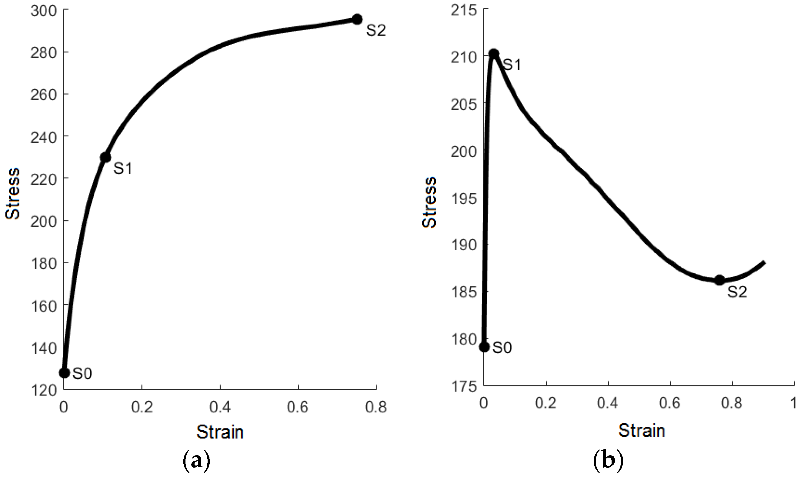
Now, the procedure followed in order to obtain the five constitutive parameters of this new law (σ₂, a, b, c, d and n) is explained. In order to select the parameters shown in Equation (1), firstly, it is necessary to observe the behaviour of the flow rule (see Figure 1). Figure 1a shows how the stress-strain curve is always growing and it is named as Case 1. This case takes place when the material is usually deformed at room temperature. Adversely, as can be observed in Figure 1b, the stress-strain curve reaches a maximum value of stress after which it decreases down to a point in which it may remain constant or a new increase of the curve may even occur. This second case is named as Case 2. In general, this second case corresponds with materials which are deformed at high temperature. In function of the type of curve that takes place, Case 1 or Case 2, the parameters are calculated.

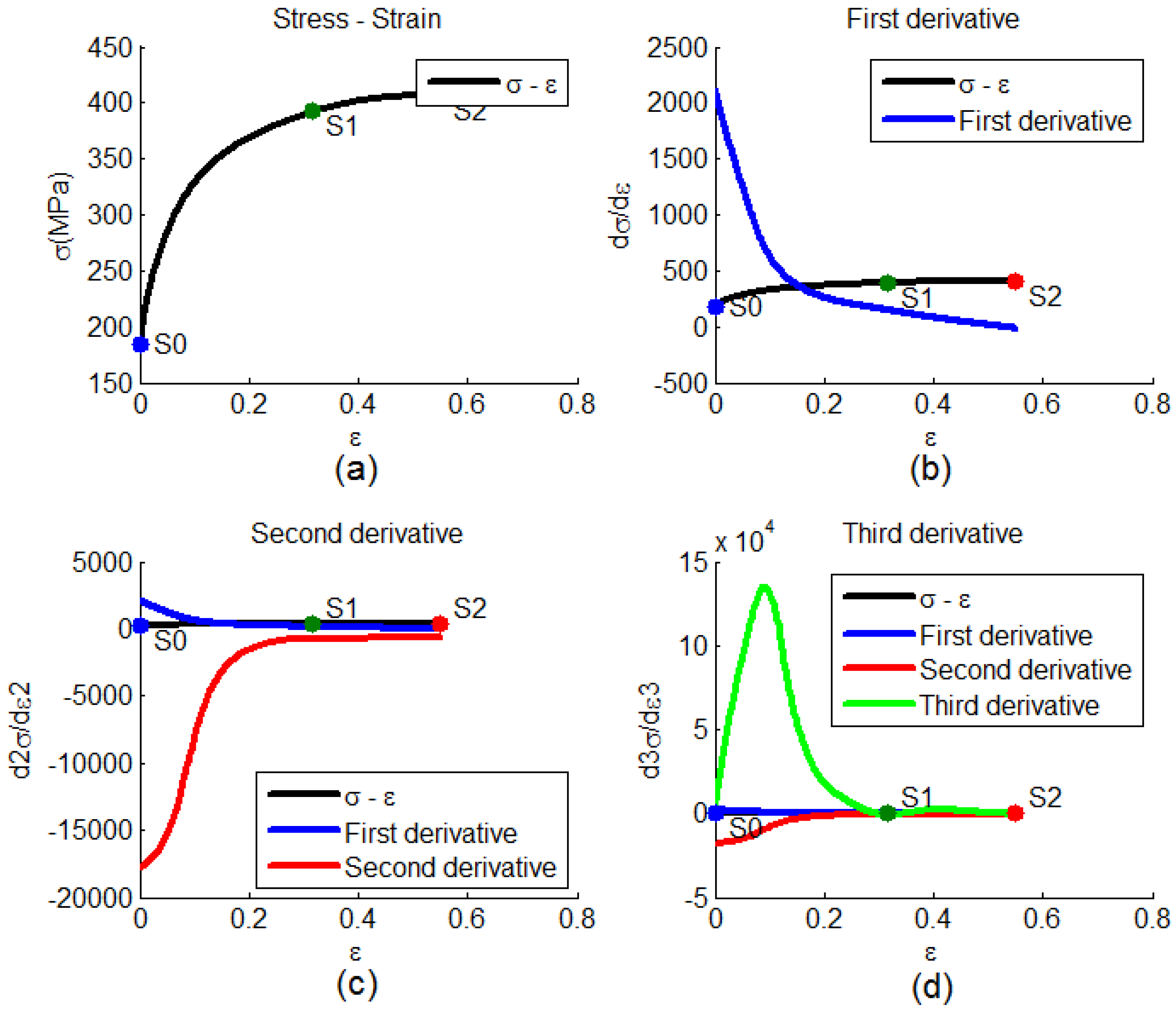
The first step is to locate the three characteristic points from the experimental curve (S₀, S₁ and S₂), which are shown in Figure 1. Each of these three points is obtained depending on the study case (Case 1 or Case 2). When Case 1 is selected, the S₀ point corresponds with the yielding point. The S₁ point corresponds with the point where the change in the curve tendency occurs and it is calculated from the third derivative of the stress-strain curve. This derivative may be numerically calculated from the experimental data of the stress-strain curves. Figure 2 shows the stress-strain curve as well as its three corresponding derivatives: first, second and third. Finally, the S₂ point is taken before barrelling happens, which may be determined since a variation in the slope of the stress-strain curve is observed.

For Case 2, the procedure followed in order to calculate the three characteristic points (S₀, S₁ and S₂) is outlined as follows. The S₀ point continues to be the yielding point. The S₁ point corresponds with the stress highest value and the S₂ with the lowest one before a change in the tendency for the stress-strain curve is observed, where this means that the curve starts to increase and therefore, barrelling begins.

Once the characteristic points are obtained from the stress-strain curve, the above-mentioned parameters (a, b, c, d and n) from Equation (1) are calculated. In order to calculate d and n, a least squares fitting is performed taking different values of these within a specific interval. The range of values for d and n that is considered in this study is as follows: 0.1 ≤ d ≤ 3.1 and 0.1 ≤ n ≤ 10.1. The variation in d and n is carried out by increments of 0.1. It may be pointed out that the ranges considered can be widened with no loss of generality. For each pair of values d and n, values for a, b and c are found by solving a system of equations which establishes that the flow rule considered has to pass through the previously selected three characteristic points (S₀, S₁ and S₂). The pair of values for d and n which gives the lowest value for the mean squared error (as Equation (4) shows) will be that selected and, therefore, the parameters a, b and c from Equation (1) will also be determined.

$$\min \left\{\mathrm{MSE}\right\}=\min \left\{\frac{1}{N}{{\displaystyle \sum _{j=1}^N({\mathsf{\sigma }}_j-{\widehat{\mathsf{\sigma }}}_j)}}^2\right\}$$

(4)

The values of the parameters obtained for the new flow rule proposed in the case of the three aluminium alloys considered in this present study and along with their different work intervals will be shown in the sections below.

3. Experimental Set-Up

In order to validate the flow rule proposed in this present research work, an experimental study of three aluminium alloys with different starting states is to be carried out, as is shown in

Table 1. Aluminium alloys and starting states under consideration.

Aluminium Alloy	Starting State
	N0	N2	N2 + TT	N4
AA5754	X	X	X	-
AA5083	X	X	X	-
AA3103	X	X	-	X

. The aluminium alloys under consideration are as follows: AA5754, AA3103 and AA5083. The different starting states studied are: N0, N2, N2 + TT and N4. N0 represents the annealed initial state. In the N2 state, the aluminium alloy is subjected to a severe plastic deformation using the ECAP (Equal Channel Angular Pressing) process which consists of two passages with route C (where this means rotating the billet 180° after each ECAP passage). In the N2 + TT state, after having ECAP-processed the material twice, a recovery thermal treatment is carried out, where this consists in heating the material up to 300 °C with a heating slope of 12 °C/min. In the N4 state, the aluminium alloy undergoes four ECAP passages with route Bc, which consists in rotating the billet 180°, 90° and 180°, respectively, after each passage.

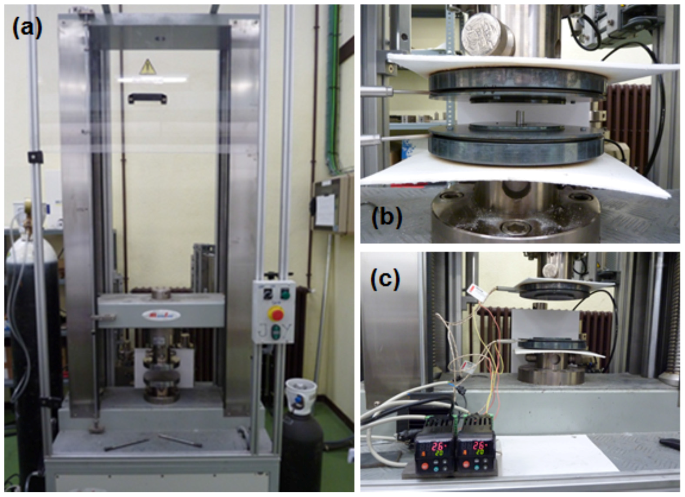
In order to perform the experimental tests, a universal testing machine, which belongs to the Public University of Navarre, Spain (see Figure 3a), was used. To carry out the compression test of the billets, it was necessary to design and to manufacture the plane-shape dies shown in Figure 3b. Finally, a set of electrical resistances was employed in order to be able to perform the compression tests isothermally. With the aim of increasing the heat flow towards the inner part of the dies and, specifically, at the contact zone with the test billet, a steel sheet was attached to the outer part of the resistances, as can be observed in Figure 3c. In this way, it is possible to carry out tests at higher temperature values, as the convection heat evacuation outwards is lower. The resistance temperature is controlled by two thermocouples, which are in contact with each of the two dies. This temperature value may be modified by the two digital PDI controllers, which are shown in Figure 3c. Once the test temperature for the resistances is programmed, the billet temperature is monitored by an external digital thermocouple until the moment when the billet reaches the desired stationary temperature value. Subsequently, the billet is placed in the proper position and it is maintained between the plane-shape dies, as is shown in Figure 3b, until it reaches the same temperature value as the dies and thus, to perform an isothermal compression test. By following this procedure it means there is a higher degree of test temperature control during the deformation process.

In order to obtain the load-stroke curve for all the aluminium alloys under consideration, six different test temperature values (25 °C, 100 °C, 150 °C, 200 °C, 250 °C and 300 °C) were studied at a compression velocity of 60 mm/min. In order to carry out this experimental study, cylindrical billets with a diameter of 8 mm and a length of 16 mm were employed. These billets are placed on the lower die and both the billet and the die are lubricated with Teflon^®. In the case of the tests at a temperature higher than 25 °C, the billet is maintained on the lower die during five minutes so that the billet may reach the same temperature as the dies and thus, the compression is isothermal.

Once the compression tests for the different aluminium alloys are carried out at the different temperature values selected, the load-stroke curve obtained for each of them is transformed into a stress-strain curve, as a previous step to the attainment of, on the one hand, Hollomon’s and Voce’s laws and, on the other hand, the new flow rule proposed in this research work.

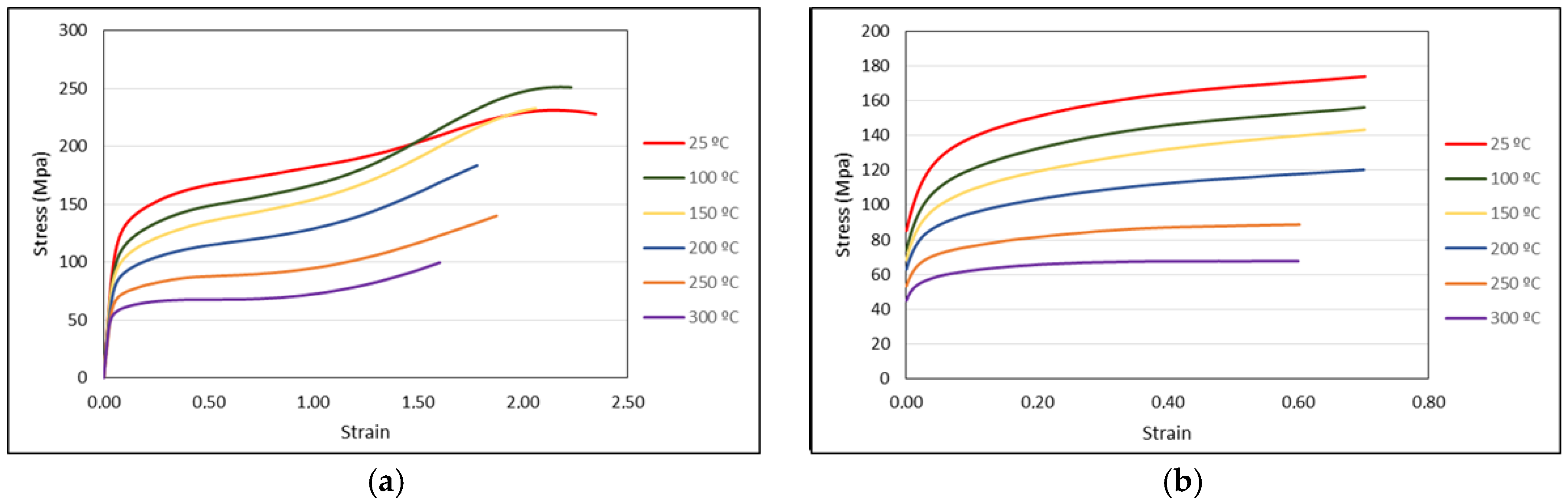
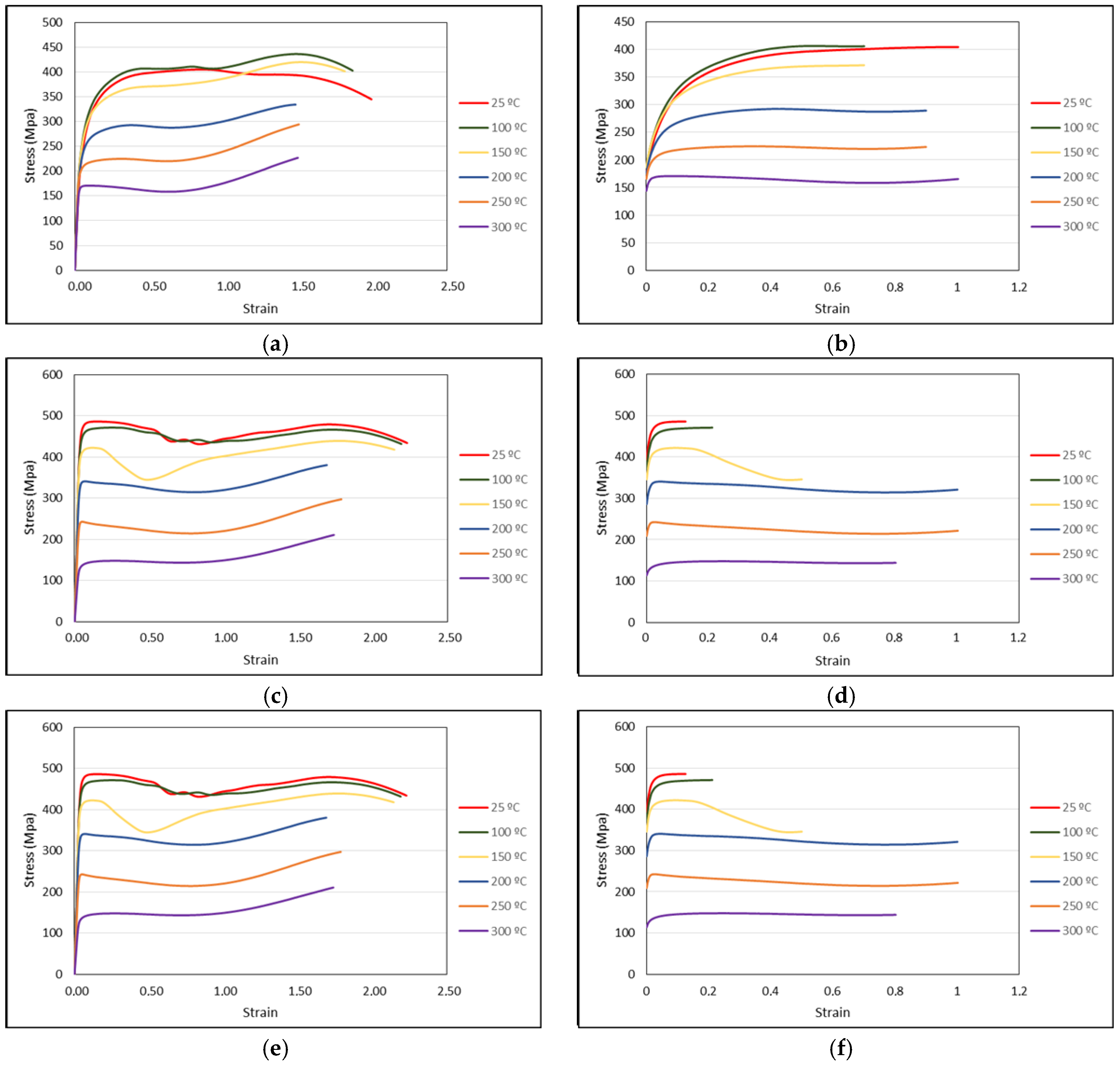
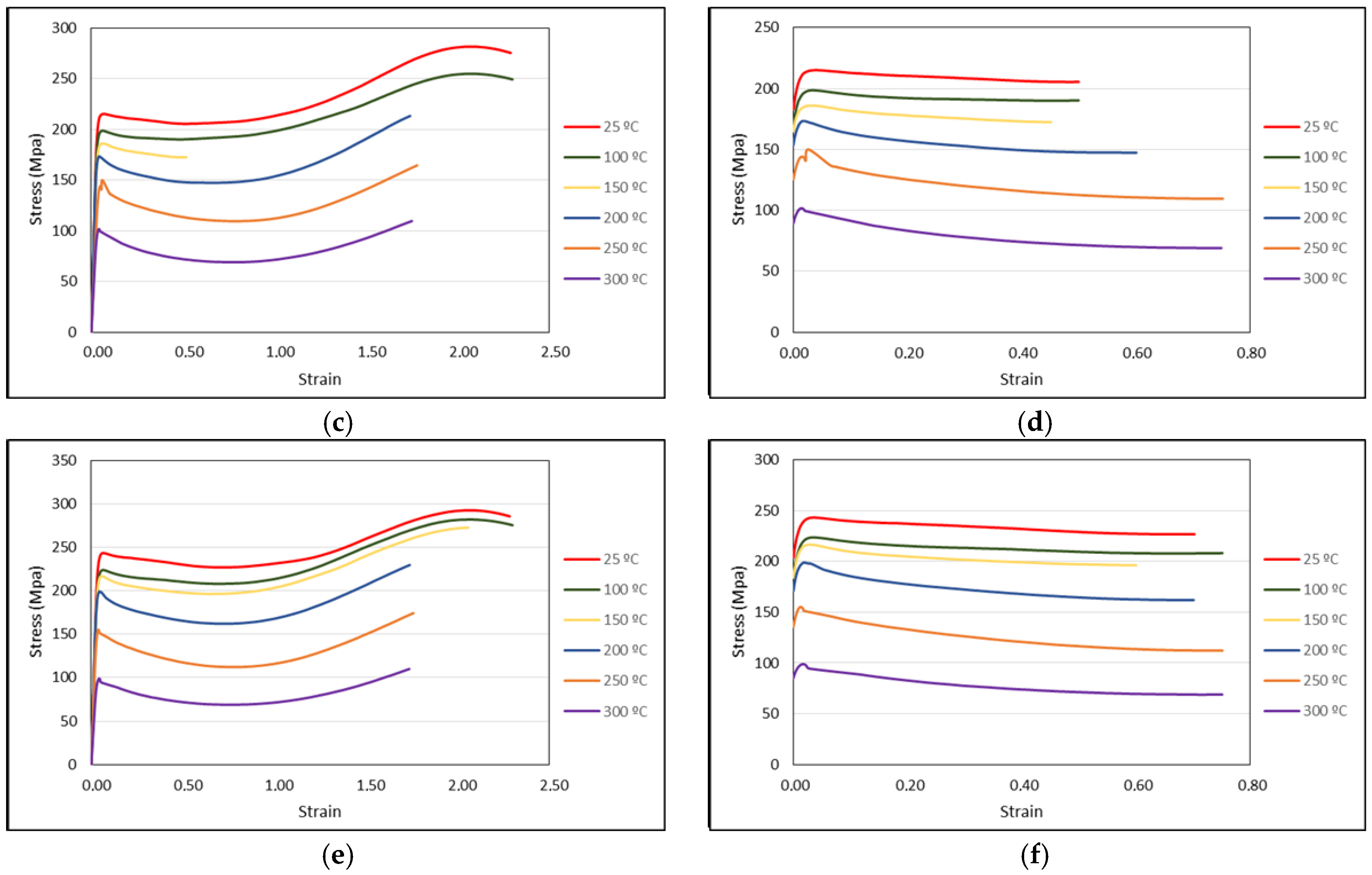
Figure 4a,c,e shows the complete stress-strain curves for AA3103 taking into account the barrelling effect that the billet undergoes when it is compressed, whereas Figure 4b,d,f shows the selected zone of the experimental curves. From this selected zone, the three flow rules under consideration are assessed. The cutting zone is established at a strain value of 0.7 although there are several cases for the ECAP-processed material where this cutting zone is lower than this former value. The reason for this is due to the change in the existing slope in the stress-strain curve for the N2 and N4 starting materials. This slope change is because of the recrystallization process, which takes place in the material at some specific temperature values, as well as the barrelling effect due to friction.

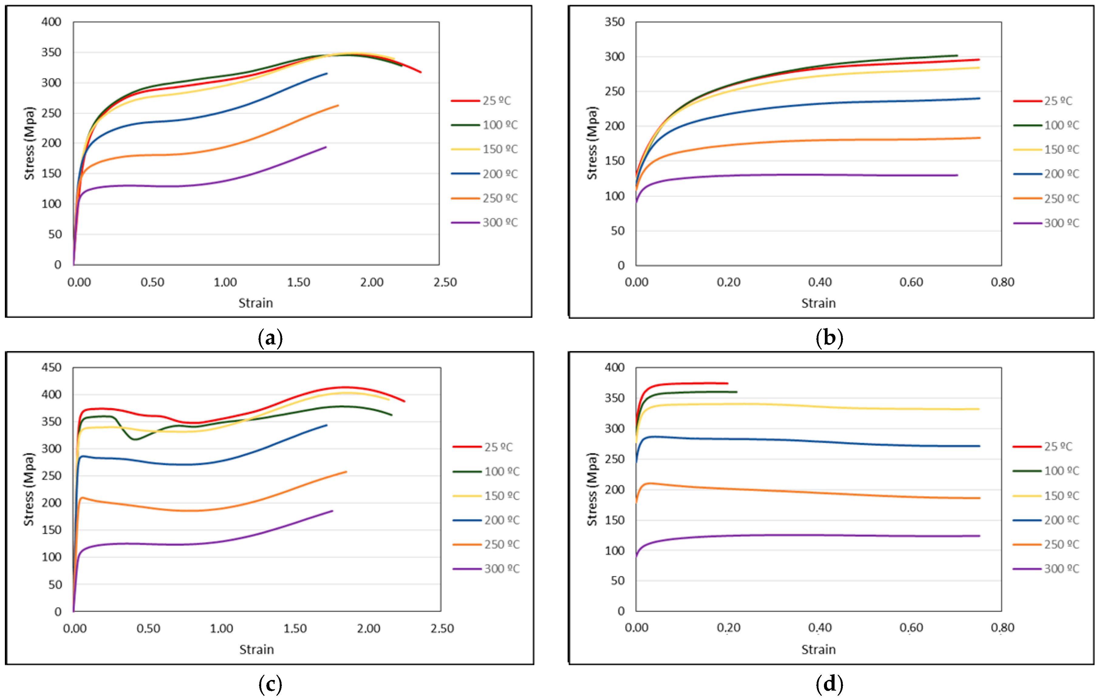
Figure 5a,c,e shows the stress-strain curves obtained for AA5754 from the experimental compression tests between plane-shape dies, whereas Figure 5b,d,f shows the zones selected in order to assess the three above-mentioned flow rules in all the cases of temperatures and starting states under consideration. In addition, it may be observed that the curves at the three lowest temperature values (that is, 25 °C, 100 °C, and 150 °C) are closer to each other than the other three remaining ones (200 °C, 250 °C, and 300 °C). This is due to the temperature effect on the material strength, which is more significant above 150 °C.

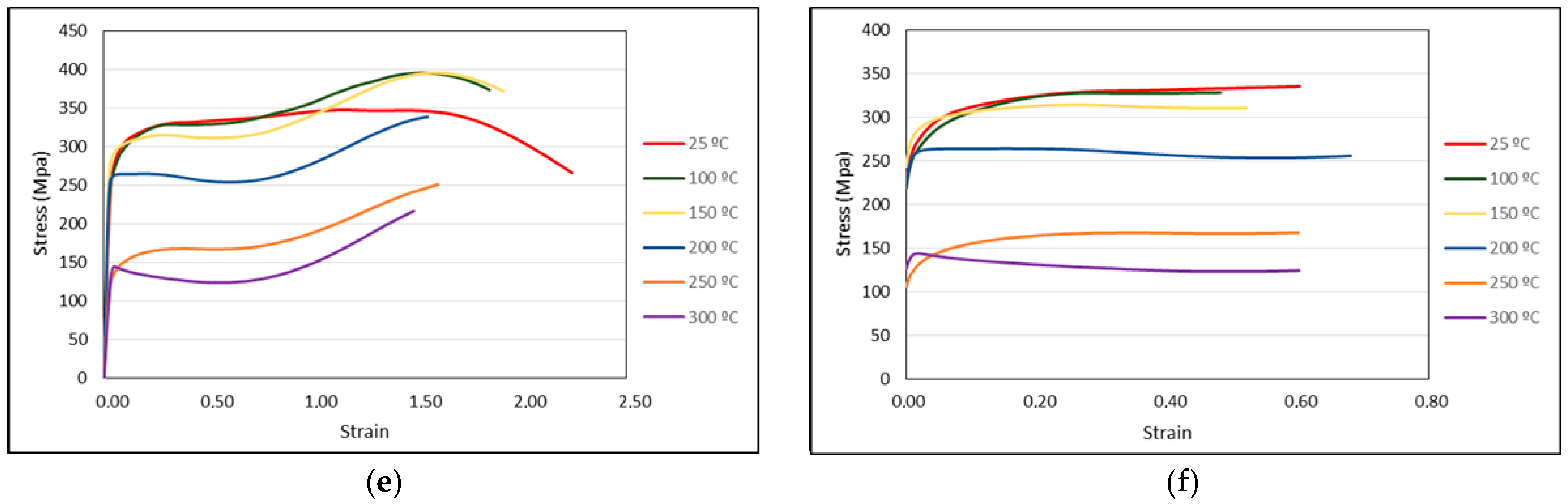
Finally, the stress-strain curves for AA5083 at its three starting states can be observed in Figure 6a,c,e. Just as occurs with AA5754, the curves at 25 °C and at 100 °C show a similar behaviour, whereas, from a temperature of 150 °C, a change in their behaviour is observed since the stress-strain curves are found to be more spaced out.

From the flow curves shown in Figure 4, Figure 5 and Figure 6 and following the previously-mentioned procedure, it is possible to obtain the parameters to be considered in Equation (1). These parameters are shown in

Table 2. Values of the parameters for the new flow rule proposed for AA3103.

Aluminium Alloy		T	a	b	c	d	n	σ2
AA3103	N0	25 °C	−88.69	98.67	3.51 × 10−4	1.00	2.30	173.95
		100 °C	−82.03	91.28	2.55 × 10−4	0.50	2.30	156.16
		150 °C	−74.79	83.22	3.17 × 10−4	0.00	2.30	143.32
		200 °C	−57.23	63.68	4.66 × 10−5	0.20	2.30	120.29
		250 °C	−35.39	41.21	3.85 × 10−5	1.70	2.30	88.76
		300 °C	−22.71	26.47	1.58 × 10−5	5.80	2.30	67.74
	N2	25 °C	−22.23	35.35	5.68 × 10−5	5.10	2.00	205.47
		100 °C	−21.14	47.21	1.84 × 10−5	10.10	2.10	190.01
		150 °C	−7.29	35.68	3.38 × 10−5	7.40	2.10	172.39
		200 °C	6.48	23.91	1.95 × 10−5	6.20	2.00	147.38
		250 °C	16.14	6.86	3.35 × 10−4	3.70	1.50	109.48
		300 °C	20.50	23.53	8.35 × 10−6	5.40	2.10	69.04
	N4	25 °C	−22.74	42.76	3.88 × 10−5	3.60	2.00	226.84
		100 °C	−21.23	41.85	5.63 × 10−5	4.80	2.00	207.86
		150 °C	−11.99	38.09	4.67 × 10−5	5.70	2.00	196.30
		200 °C	9.28	23.25	3.95 × 10−5	4.50	1.90	162.10
		250 °C	23.76	22.80	8.35 × 10−6	4.30	2.00	112.16
		300 °C	16.57	25.56	1.28 × 10−5	5.20	2.10	68.79

,

Table 3. Values of the parameters for the new flow rule proposed for AA5754.

Aluminium Alloy		T	a	b	c	d	n	σ2
AA5754	N0	25 °C	−163.13	193.85	1.58 × 10−4	3.00	2.40	295.83
		100 °C	−180.77	201.12	4.59 × 10−4	1.40	2.30	301.55
		150 °C	−161.73	176.34	2.20 × 10−4	2.30	2.30	284.18
		200 °C	−122.26	129.52	3.49 × 10−4	0.90	2.20	240.09
		250 °C	−74.40	78.76	1.15 × 10−4	2.40	2.20	183.48
		300 °C	−38.34	−184.75	−3.01	5.50	0.30	129.42
	N2	25 °C	−68.93	69.12	1.08 × 10−4	0.00	2.00	374.16
		100 °C	−66.90	67.07	1.28 × 10−4	0.00	2.00	360.10
		150 °C	−53.94	67.81	7.18 × 10−1	1.30	0.20	331.96
		200 °C	−26.43	44.62	3.87 × 10−5	2.70	2.00	271.41
		250 °C	−7.03	5.00	1.24 × 10−1	0.50	0.10	186.13
		300 °C	−33.85	46.69	6.66 × 10−1	4.80	0.40	123.75
	N2 + FLASH	25 °C	−101.55	132.66	3.26 × 10−5	4.80	2.30	334.13
		100 °C	−108.90	252.73	1.45	4.20	0.40	328.35
		150 °C	−67.27	129.40	1.09	2.90	0.30	310.74
		200 °C	−28.76	27.61	4.04 × 10−1	1.60	0.20	253.46
		250 °C	−61.03	94.76	8.82 × 10−1	2.30	0.40	166.69
		300 °C	3.37	21.48	4.29 × 10−5	5.00	2.00	123.35

and

Table 4. Values of the parameters for the new flow rule proposed for AA5083.

Aluminium Alloy		T	a	b	c	d	n	σ2
AA5083	N0	25 °C	−226.36	226.16	3.53 × 10−4	3.10	2.30	404.78
		100 °C	−221.66	1287.65	4.37	4.60	0.50	406.14
		150 °C	−185.25	4962.15	2.27 × 101	4.40	0.40	371.96
		200 °C	−112.88	607.28	2.95 × 101	3.70	0.40	292.66
		250 °C	−53.91	−541.05	−5.52	4.00	0.30	219.96
		300 °C	−14.17	52.99	6.65 × 10−6	4.50	2.20	158.37
	N2	25 °C	−92.03	92.61	9.26 × 10−5	8.70	2.00	485.91
		100 °C	−98.15	114.76	4.44 × 10−5	9.20	2.10	471.28
		150 °C	1.74	131.41	1.72 × 10−1	6.30	0.70	344.50
		200 °C	−27.98	58.86	5.09 × 10−5	2.50	2.00	314.38
		250 °C	−4.96	36.99	2.44 × 10−5	3.10	2.00	214.34
		300 °C	−29.08	34.05	5.48 × 10−1	1.90	0.30	143.21
	N2 + FLASH	25 °C	−235.76	−1508.98	−5.37	5.3	0.6	388.85
		100 °C	−217.70	269.52	1.81 × 10−4	4.7	2.5	379.35
		150 °C	−170.90	203.08	1.01 × 10−4	4.9	2.4	326.85
		200 °C	−109.13	193.92	0.93	3.2	0.5	255.71
		250 °C	−52.90	116.07	1.09	2.9	0.4	178.89
		300 °C	−15.21	17.16	0.53	1.5	0.2	118.31

for AA3103, AA5754 and AA5083, respectively, where these alloys may be without any previous deformation or after having been previously ECAP-processed.

4. Determination of the Parameters for Hollomon’s and Voce’s Flow Rules

From the zones selected in the stress-strain curves obtained experimentally, flow rules type Hollomon (Equation (2)) and Voce (Equation (3)) were previously fitted in order to determine their accuracy level in relation to the new flow rule proposed.

Table 5. Values for Hollomon’s parameters in the case of AA3103.

T	AA3103
	N0		N2		N4
	k	n	k	n	k	n
25 °C	183.34	1.24 × 10−1	208.62	−3.13 × 10−3	229.99	−1.11 × 10−2
100 °C	164.10	1.33 × 10−1	192.34	−1.25 × 10−3	209.87	−1.21 × 10−2
150 °C	149.46	1.36 × 10−1	173.58	−1.33 × 10−2	197.42	−1.88 × 10−2
200 °C	124.70	1.15 × 10−1	146.86	−3.51 × 10−2	163.43	−4.19 × 10−2
250 °C	93.63	8.72 × 10−2	110.48	−6.08 × 10−2	116.18	−5.93 × 10−2
300 °C	71.42	6.21 × 10−2	69.47	−7.61 × 10−2	69.95	−6.72 × 10−2

,

Table 6. Values for Hollomon’s parameters in the case of AA5754.

T	AA5754
	N0		N2		N2 + FLASH
	k	n	k	n	k	n
25 °C	327.42	1.61 × 10−1	386.78	1.91 × 10−2	354.10	6.34 × 10−2
100 °C	330.16	1.64 × 10−1	376.49	2.31 × 10−2	357.81	7.65 × 10−2
150 °C	311.59	1.48 × 10−1	351.82	1.86 × 10−2	321.42	2.76 × 10−2
200 °C	257.68	1.14 × 10−1	286.62	5.66 × 10−3	259.88	−1.38 × 10−3
250 °C	191.84	7.31 × 10−2	190.57	−2.39 × 10−2	179.47	7.54 × 10−2
300 °C	137.63	4.71 × 10−2	133.45	4.88 × 10−2	124.10	−3.52 × 10−2

and

Table 7. Values for Hollomon’s parameters in the case of AA5083.

T	AA5083
	N0		N2		N2 + FLASH
	k	n	k	n	k	n
25 °C	439.03	1.43 × 10−1	494.96	1.56 × 10−2	183.34	1.24 × 10−1
100 °C	450.21	1.39 × 10−1	485.35	2.10 × 10−2	164.10	1.33 × 10−1
150 °C	406.85	1.19 × 10−1	406.71	−1.58 × 10−3	149.46	1.36 × 10−1
200 °C	317.66	8.29 × 10−2	322.10	−1.37 × 10−2	124.70	1.15 × 10−1
250 °C	235.04	3.86 × 10−2	218.86	−2.72 × 10−2	93.63	8.72 × 10−2
300 °C	163.14	−1.05 × 10−2	149.12	1.93 × 10−2	71.42	6.21 × 10−2

show the values obtained for Hollomon’s law in the cases of AA3103, AA5754 and AA5083, respectively, and for all the starting states under consideration.

Table 8. Values for Voce’s parameters in the case of AA3103.

T	AA3103
	N0			N2			N4
	m	B	a	m	B	a	m	B	a
25 °C	−12.97	165.19	85.58	−122.02	215.65	183.31	−63.46	239.98	231.34
100 °C	−11.60	147.53	74.86	−133.57	198.72	169.00	−74.74	223.25	217.04
150 °C	−10.35	134.95	70.30	−141.26	186.29	161.63	−137.68	216.19	185.01
200 °C	−11.91	113.74	64.70	−256.57	167.99	153.59	−142.37	201.10	171.45
250 °C	−15.24	86.50	54.54	−137.29	145.78	126.15	−163.09	156.38	137.48
300 °C	−23.59	66.55	45.49	−149.94	103.52	89.74	−142.78	99.83	86.24

,

Table 9. Values for Voce’s parameters in the case of AA5754.

T	AA5754
	N0			N2			N2 + FLASH
	m	B	a	m	B	a	m	B	a
25 °C	−10.58	284.07	129.86	−91.15	372.94	315.76	−26.38	323.46	229.32
100 °C	−10.19	290.74	124.25	−88.53	358.90	298.36	−22.91	320.79	218.89
150 °C	−12.28	271.13	126.32	−100.24	339.15	289.23	−46.45	309.64	257.12
200 °C	−15.59	229.36	122.83	−148.86	284.91	251.43	−145.11	262.13	224.69
250 °C	−21.56	176.78	114.25	−129.96	210.88	183.50	−21.23	164.24	106.01
300 °C	−36.83	128.51	94.05	−34.69	123.65	93.22	−131.82	145.25	126.86

and

Table 10. Values for Voce’s parameters in the case of AA5083.

T	AA5083
	N0			N2			N2 + FLASH
	m	B	a	m	B	a	m	B	a
25 °C	−11.11	392.93	178.57	−90.93	482.71	394.50	−9.76	384.07	152.14
100 °C	−12.42	397.98	183.71	−75.38	468.82	378.72	−10.28	374.86	161.61
150 °C	−14.45	363.33	187.17	−117.86	414.30	346.07	−13.05	321.51	155.54
200 °C	−21.98	286.89	175.66	−128.49	340.14	286.81	−17.77	250.86	145.56
250 °C	−43.71	221.88	170.54	−162.88	243.75	209.46	−28.06	179.01	125.77
300 °C	−141.06	167.68	144.43	−58.63	146.07	115.85	−106.99	121.58	103.75

show the values obtained for the parameters from Voce’s law in the case of AA3103, AA5754 and AA5083, respectively, and at all three different starting states selected.

5. Discussion of Results

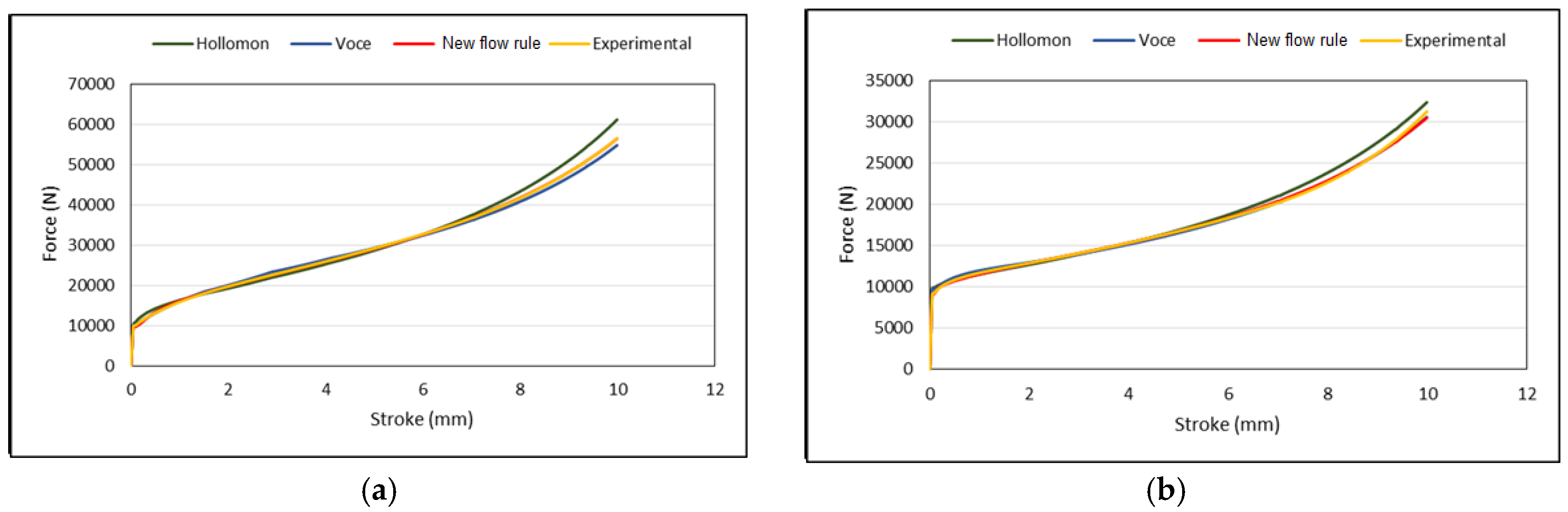
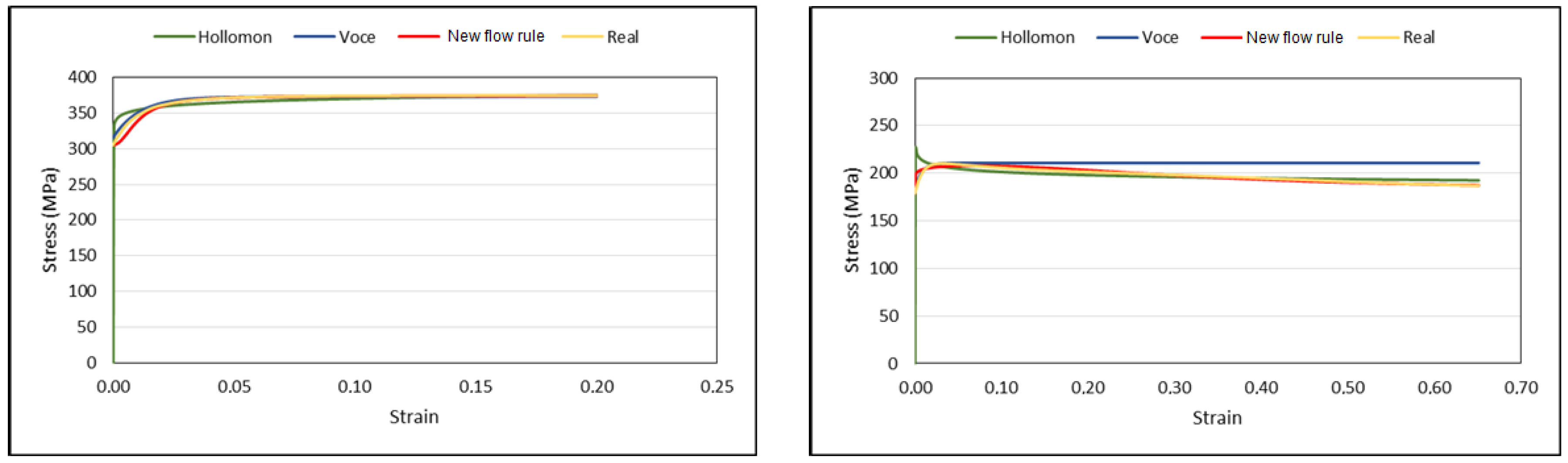
Once the experimental procedures used have been shown, the results obtained in the present research work are now outlined in this section. First of all, Figure 7 shows the approach which the three flow rules present both at low (25 °C) and at high (250 °C) temperature in relation to the experimental stress-strain curve. It may be observed that, at low temperature, the approach is acceptable for Hollomon’s and Voce’s laws and it is very good for the new law proposed, as it is practically superimposed on the experimental curve. Nevertheless, at a temperature of 250 °C, where dynamic recrystallization takes place for the previously ECAP-processed material, the curve corresponding with Hollomon’s law increases up to a stress value of 240 MPa (about 40 MPa above the experimental curve) and then undergoes a sudden decrease which crosses the experimental curve at about a strain value of 0.04. On the other hand, the curve corresponding with Voce’s flow rule reaches the same maximum stress value as that from the experimental curve but then remains constant as strain increases, where this means that the approach seems not to be good enough either, as will be numerically demonstrated below. However, although the new law proposed does not show such a very good approach as found at low temperature values, the approach along the decreasing part is good enough. Therefore, it may be concluded that the approach of this new law to reality is very good and, thus, much better than in the cases of both Hollomon’s and Voce’s laws.

With the aim of quantifying the precision of fit between the different flow rules studied here and the true behaviour of the material during the compression test between plane-shape dies, the root mean square error (RMSE) was assessed in each of the experiments with the three aluminium alloys under consideration, as is depicted in Equation (5).

$$\mathrm{RMSE}=\sqrt{\frac{1}{N}{\displaystyle \sum _{j=1}^N{\left({\mathsf{\sigma }}_j-{\widehat{\mathsf{\sigma }}}_j\right)}^2}}$$

(5)

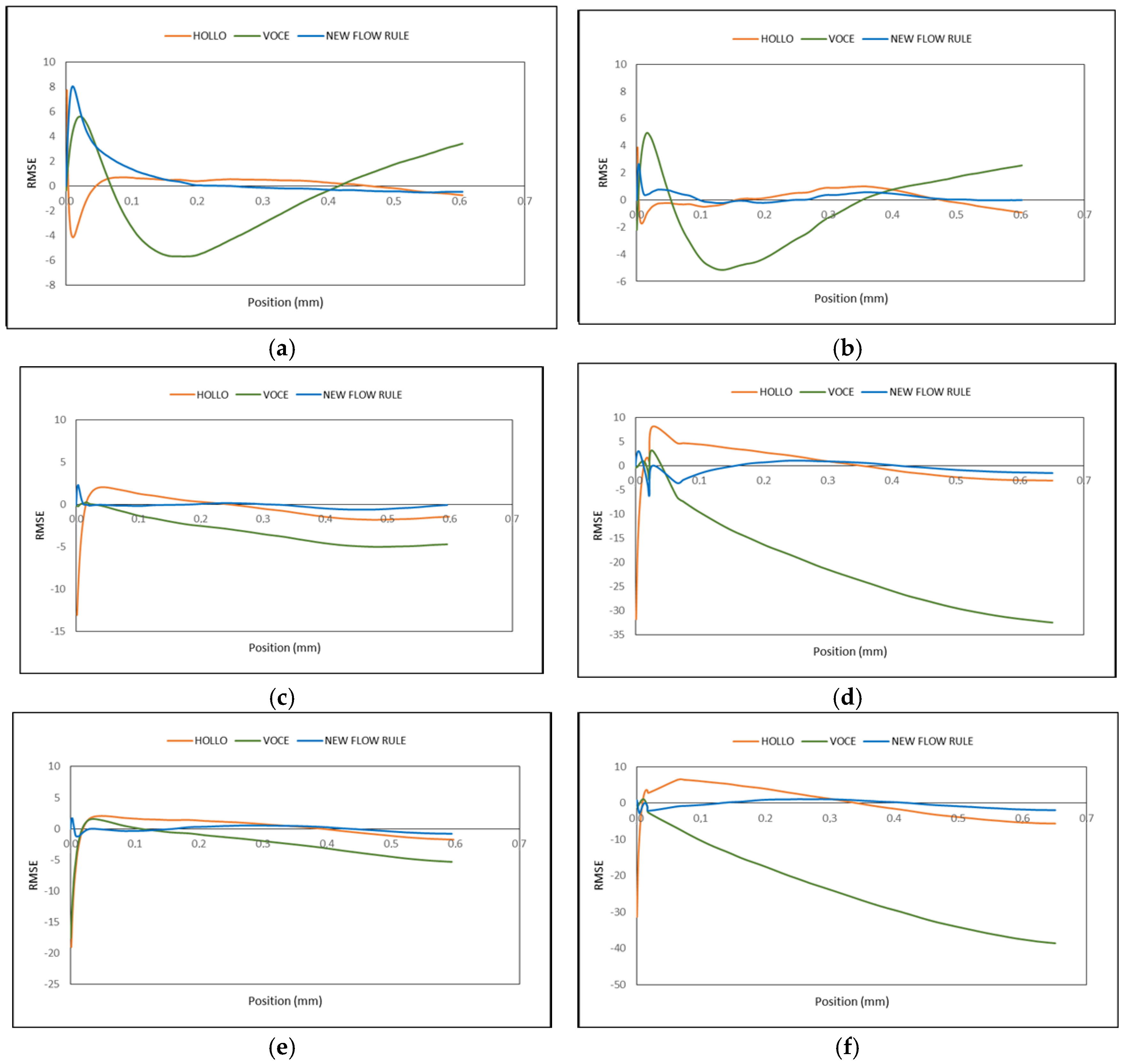
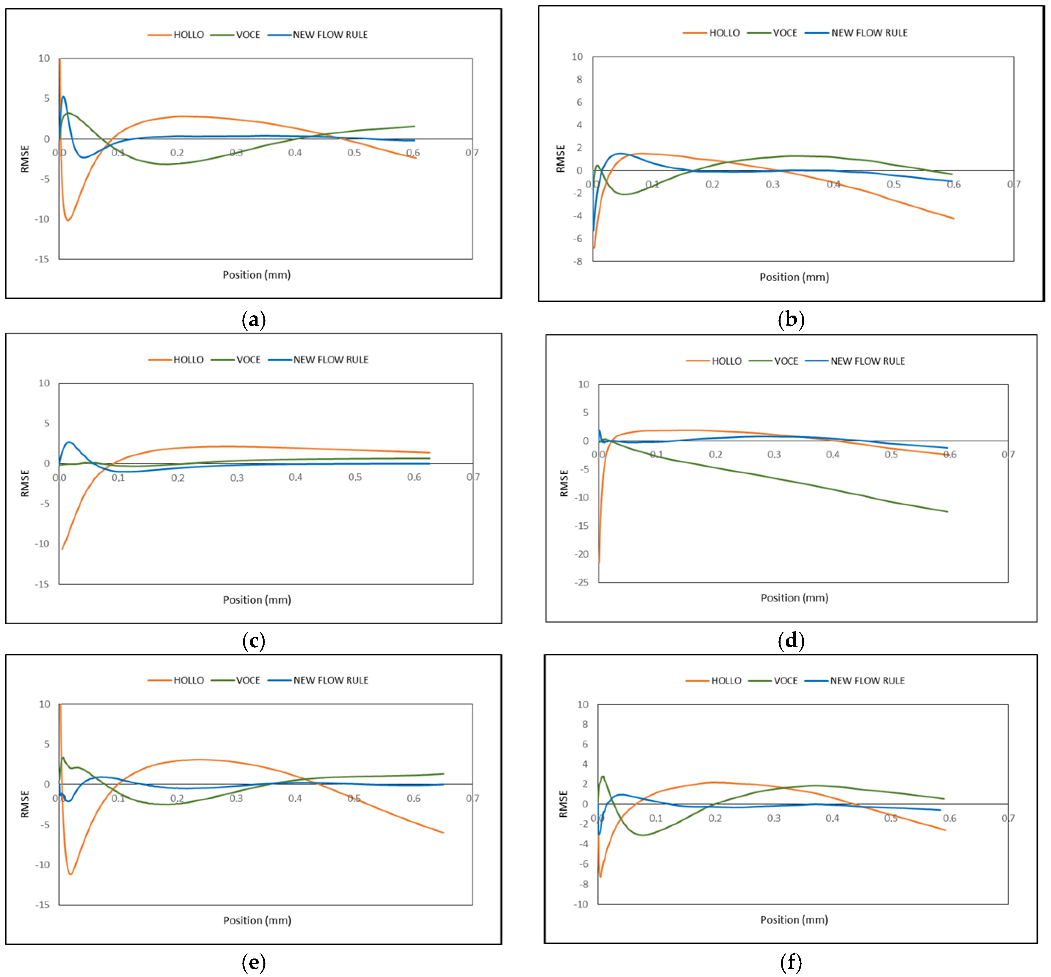
For AA3103, as can be observed in Figure 8, the flow rule proposed fits the behaviour of the alloy better in the temperature range considered. Moreover, it is observed that Voce’s flow rule is that with the highest values for RMSE. For the material with N0 state (see Figure 8a,b), the error fluctuates between positive and negative values, whereas with the ECAP-processed material (see Figure 8c–f), the error value is negative and it increases as the material is compressed, where this tendency turns out to be greater at higher temperature values. In the case of Hollomon’s flow rule, it is observed that there is a fitting which is better than in the case of Voce’s flow rule. For N0 starting state, the error value is negative at first and then turns positive and decreases as compression progresses. For N2 and N4 state starting materials (see Figure 8c–f), the error value is positive at first until it turns to negative around a strain value of 0.35. In the case of the new flow rule and for N0 state material, the error with the highest value occurs at the beginning of the compression process, whereas, as the material is being compressed, the error value decreases. For N2 and N4 starting states (Figure 8c–f), the error obtained with the new flow rule is clearly smaller than in the case of the two remaining ones. It may be stated that its approach to the experimental curve is very good, where this turns out to be better at lower temperature values, as can be observed in Figure 8c,e.

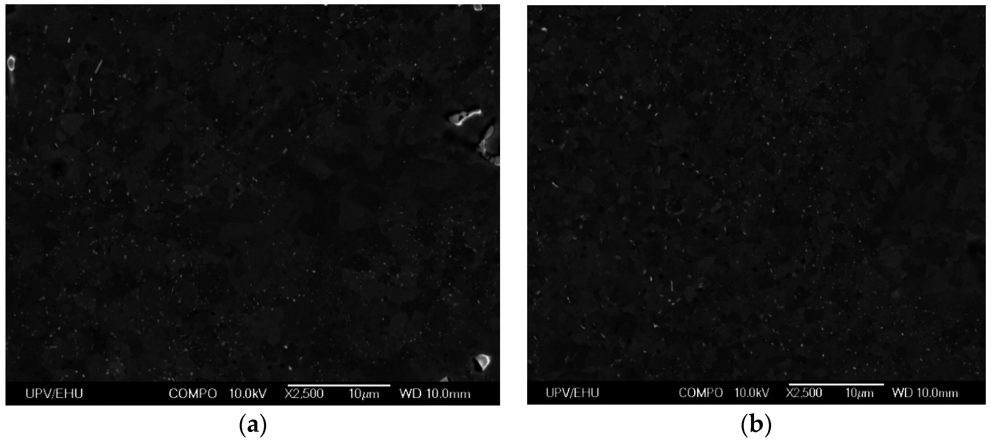
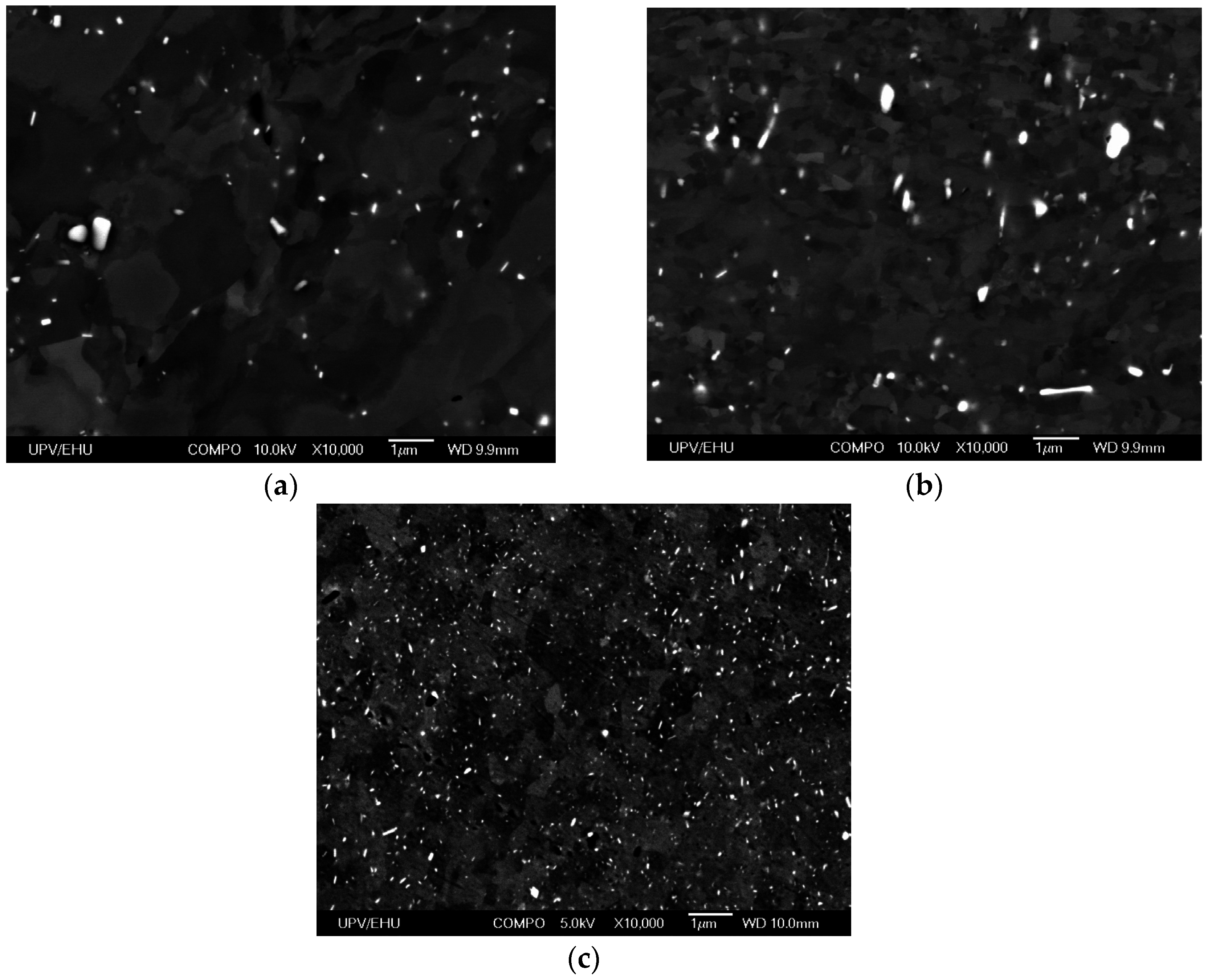
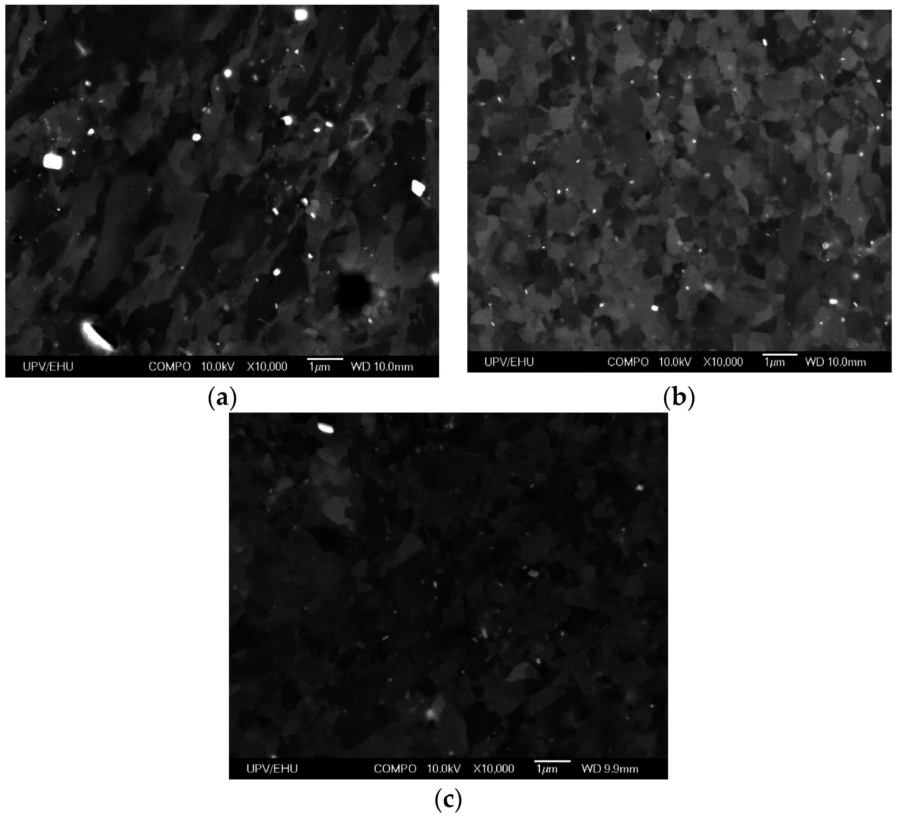
Figure 9 shows SEM (Scanning Electron Microscopy) micrographs for billets forged at 250 °C from different deformation states. As can be observed in N0 material, the grain size is bigger than in the two other cases due to a lower level of strain accumulation.

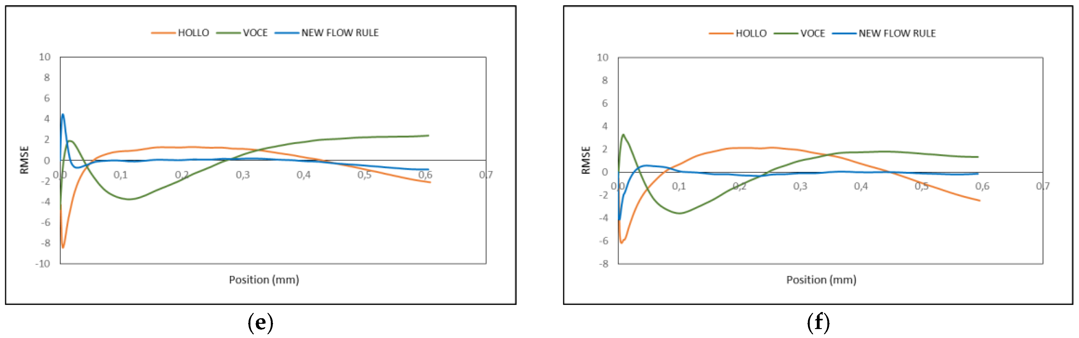
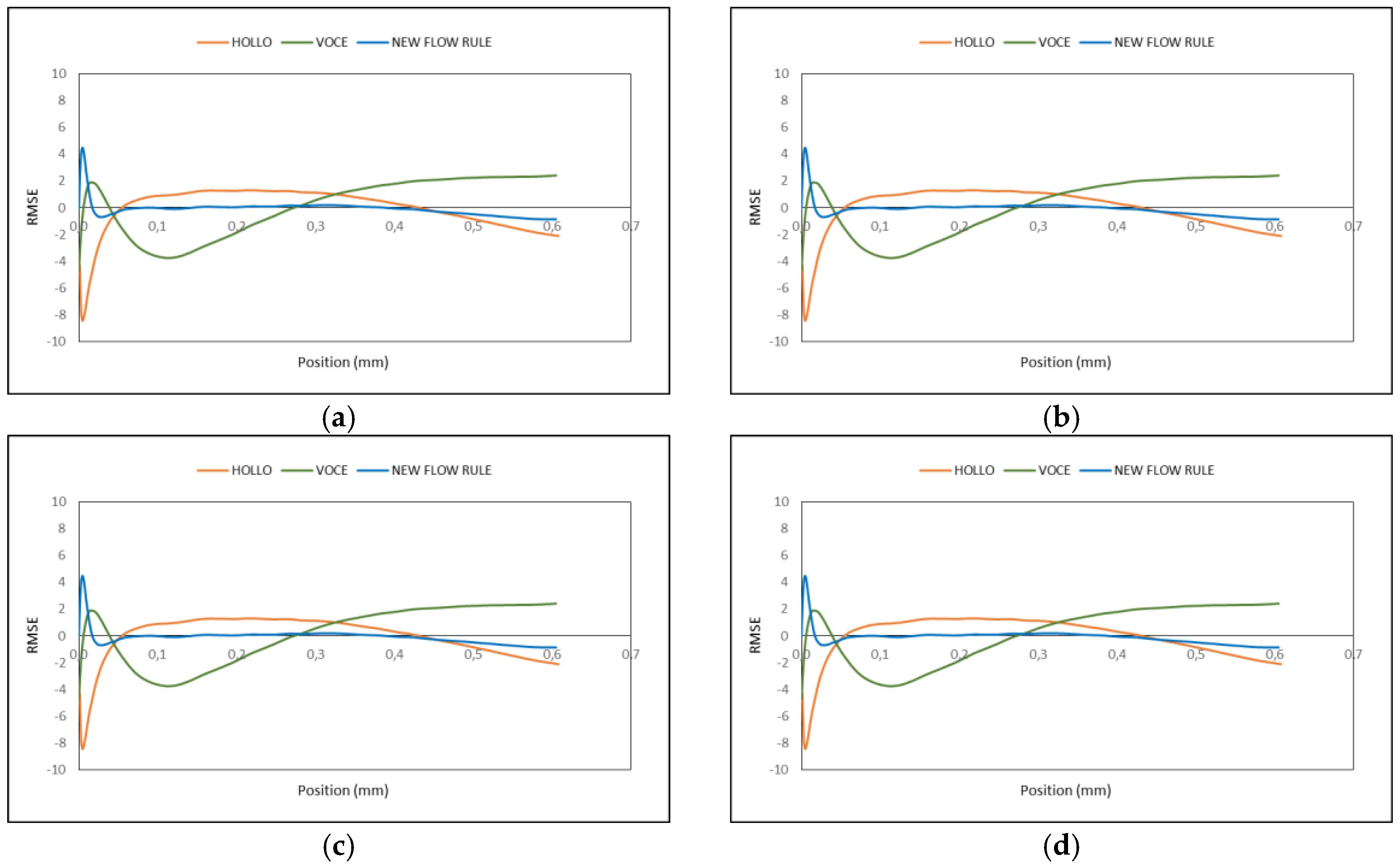
If RMSE graphs for AA5754 are analysed at the three starting states under consideration (N0, N2 and N2 + flash), it may be observed that the curve with the lowest error value (that is, with the best fitting) is that corresponding to the new flow rule (see Figure 10). In the case of Hollomon’s flow rule, it may be observed in Figure 10a that for N0 state at low temperature, the error shows a behaviour which is the contrary to that of Voce’s flow rule. For N2 starting state at low and high temperature (see Figure 10c,d) as well as for N2 + flash starting state at high temperature (see Figure 10f), the error graph from Hollomon’s flow rule is similar. Nevertheless, for N2 + flash starting state at low temperature (see Figure 10e), the curve is similar to that from N0 at low temperature (see Figure 10a). In the case of Voce’s flow rule, it is observed in Figure 10d that for N2 starting material at high temperature, the error graph shows the same behaviour as its equivalent from AA3103 (Figure 8d), which, at the same time, is contrary to the rest of the starting states and temperatures. This is due to the fact that the temperature value coincides with the recrystallization temperature of AA5754 for a N2 starting state. In the case of the new flow rule proposed, it may be observed that the fit to the experimental curve is better.

Figure 11 shows SEM micrographs for AA5754 billets forged at 250 °C from different deformation states. It is observed that recrystallization occurs in the previously ECAP-processed samples, as a consequence of the higher level of previous strain accumulated. Finally, with regard to the error graphs obtained from AA5083 (see Figure 12), a similar behaviour to AA5754 may be observed.

Figure 13 shows SEM micrographs for AA5083 billets forged at 250 °C from different deformation states. As in the previous case, it is observed that for previously ECAP-processed billets, recrystallization takes place because of the higher value of previous strain.

Table 11. RMSE of each flow rule obtained for AA3103 in relation to the experimental curve (MPa).

Alloy	T (°C)	N0			N2			N4
		HOLL	VOCE	NEW	HOLL	VOCE	NEW	HOLL	VOCE	NEW
AA3103	25	1.13	5.26	2.15	3.43	7.13	0.71	4.75	7.24	1.11
	100	0.67	5.04	1.21	3.23	6.43	0.64	4.1	10.17	0.79
	150	0.94	4.81	1.41	4.45	8.92	0.59	4.47	13.44	0.77
	200	0.69	3.8	0.41	4.25	14.69	0.74	5.47	28.54	1.05
	250	0.51	2.34	0.31	4.91	26.25	1.53	5.79	32.16	1.27
	300	0.85	1.23	0.15	3.5	28.25	0.65	3.75	24.63	0.71

shows the error values obtained for AA3103. It may be observed that for N0 starting state at low temperature, the best approach turns out to be for Hollomon’s flow rule followed by the new flow rule at a close distance, whereas at high temperature, the new flow rule turns out to be the best. With regard to N2 and N4 starting materials, the best approach is achieved with the new flow rule and with a significant difference in relation to Hollomon’s and Voce’s flow rules.

In the case of the error values for AA5083 (see

Table 12. RMSE of each flow rule obtained for AA5083 in relation to the experimental curve (MPa).

Alloy	T (°C)	N0			N2			N2 + Flash
		HOLL	VOCE	NEW	HOLL	VOCE	NEW	HOLL	VOCE	NEW
AA5083	25	5.71	5.16	4.39	5.99	2.15	2.67	3.76	5.27	1.78
	100	6.28	6.52	1.87	4.71	1.51	2.83	14.3	6.02	0.98
	150	5.54	5.99	1.76	9.02	3.57	3.54	4.08	4.16	1.55
	200	4.05	5.45	2.29	7.15	6.27	1.66	4.53	3.56	2.05
	250	2.64	3.7	0.93	5.23	13.87	2.11	3.05	2.96	0.67
	300	2.61	1.69	0.83	2.92	1.56	0.89	3.36	15.47	0.74

), it is observed that the new flow rule provides a better approach for all the starting states in comparison with Hollomon and Voce. The only exception occurs in the case of N2 starting material at 25 °C and at 100 °C, where Voce’s flow rule approaches better. Lastly, it should be pointed out that for this aluminium alloy, the difference in the approach between the new flow rule proposed and those from Hollomon or Voce is rather significant, as can be observed in Table 12.

Similar to what happens with AA5083, the flow rule with the best approach to the experimental curve for AA5754 is the new flow rule in all cases (see

Table 13. RMSE of each flow rule obtained for AA5754 in relation to the experimental curve (MPa).

Alloy	T (°C)	N0			N2			N2 + Flash
		HOLL	VOCE	NEW	HOLL	VOCE	NEW	HOLL	VOCE	NEW
AA5754	25	9.18	6.59	2.5	11.98	2.11	3.03	11.13	4.78	1.33
	100	9.84	7.78	2.37	8.32	2.37	1.43	10.14	4.75	1.46
	150	7.86	6.78	3.03	33.6	37.1	7.78	7.91	5.5	1.6
	200	7.34	4.35	2.24	7.36	11.57	2.4	5.54	5.49	1.68
	250	4.58	2.28	1.59	5.32	16.47	1.42	3.42	2.79	0.84
	300	3.96	3.86	1.35	3.09	1.63	0.87	2.16	1.41	0.66

). There is only one exception and it occurs with N2 starting material at 25 °C, where the best approach corresponds with Voce’s flow rule. As for AA5083, in the rest of the cases, the improvement achieved by the new flow rule in the approach to the experimental curve is rather significant in relation to Hollomon’s and Voce’s flow rules.

6. Validation by FEM

Now that the procedure followed in order to obtain the different material flow rules and the results obtained in the comparison with the experimental curve have previously been outlined, the same study is carried out by finite element modelling (FEM) with the aim of comparing the fitting of the three flow rules under consideration.

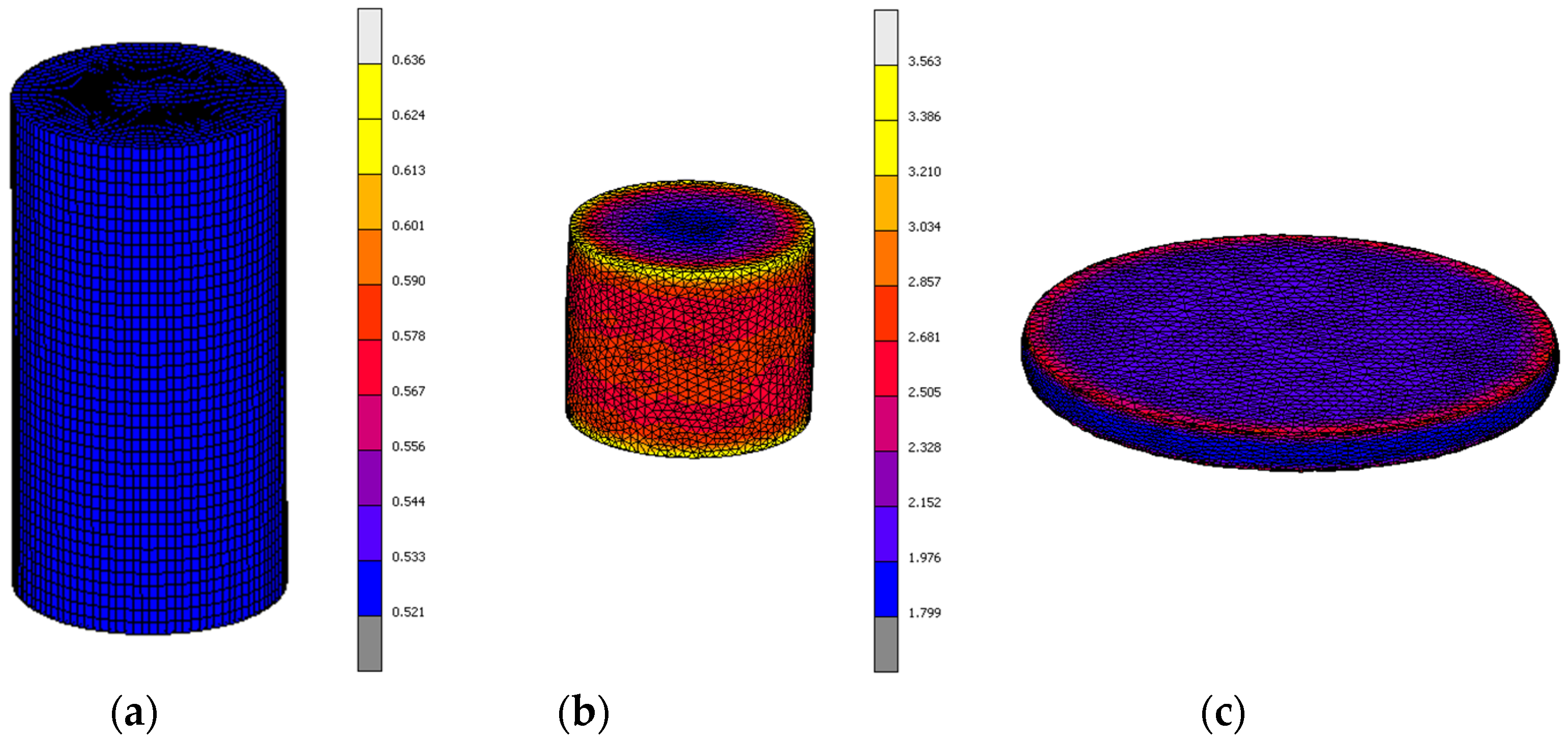
In order to do this, a model, which consists of the two plane-shape dies and the billet, is generated. A fine meshing for the billet is performed with an element size in height of 0.4 mm and a hexahedral type element with six control nodes, as can be observed in Figure 14. After this, the material flow rules with the elastic part also being included are introduced with a Young’s modulus for aluminium of 70 GPa and a Poisson’s coefficient of 0.3. Furthermore, it is necessary to indicate the experimental test temperature that is required for the simulation. Therefore, fifty-four FEM simulations are needed in order to cover all the experimental study, which analyses six temperatures, three flow rules and three starting states.

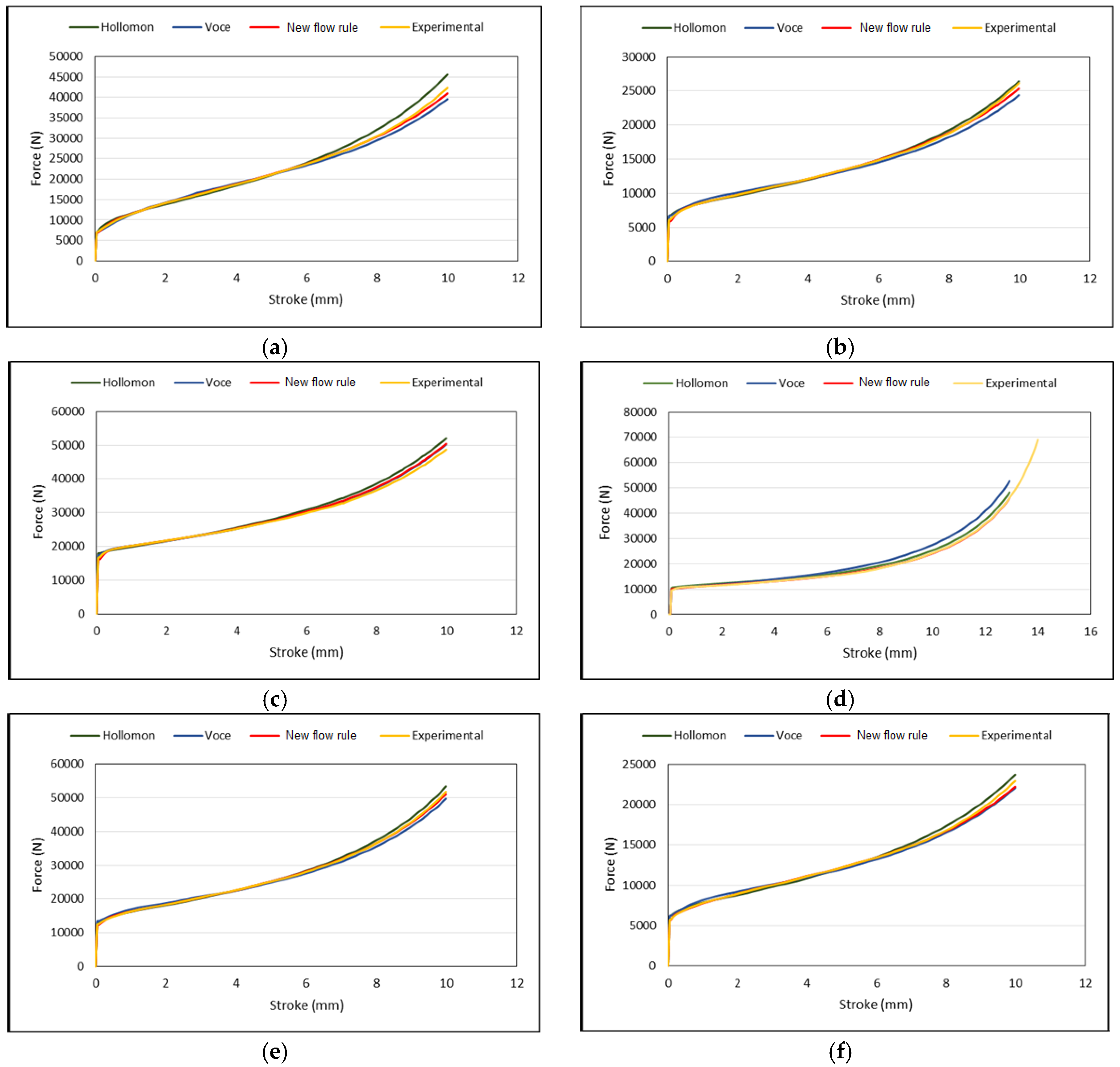
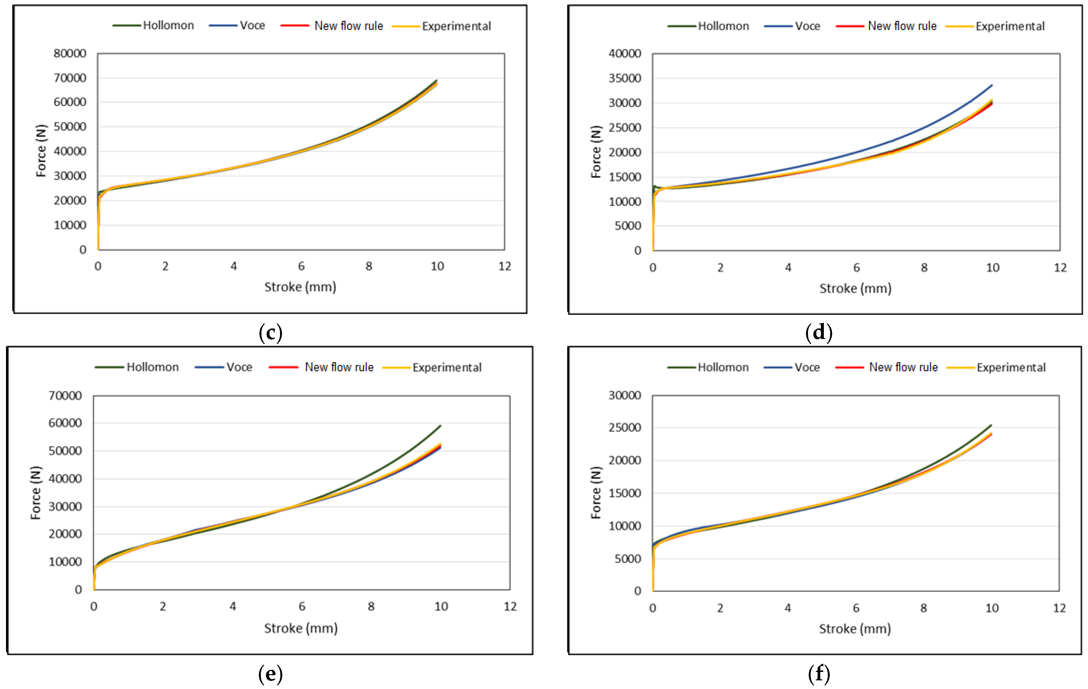
Having explained the procedure to study the process by finite element simulations, the load-stroke curves obtained both for each flow rule and for each aluminium alloy are shown below. In the case of AA3103, as is shown in Figure 15, at low temperature values, the approach of the three flow rules to the curve experimentally obtained is rather good. Only the curve from Voce’s law differs from the experimental curve as the process progresses, whereas in the cases of Hollomon’s law and the new law proposed, they follow the experimental curve very satisfactorily. Nevertheless, in the case of the starting states where the material is ECAP-processed, the approach of Voce’s law is worse and the curve with the best approach is that from the proposed new flow rule. The curve from Hollomon’s law also has a good approach but nevertheless, at the initial part, it differs from the experimental curve more than the curve, which corresponds with the new law (see Figure 15c–f).

Figure 16 shows the load-stroke curves obtained from the FEM simulations for AA5754 at the three starting states and at temperatures of 25 °C and 250 °C. It may be observed that the approach of the proposed new law is very good until the compression final part, which is the zone with the highest error value. This also happens in the cases of Hollomon’s and Voce’s laws and it is due to the barrelling effect which takes place during the compression process. For this aluminium alloy, the approach of the three laws is acceptable and only in the cases of Hollomon’s law at low temperature (see Figure 16a) and Voce’s law at high temperature and N2 state (see Figure 16d), they present appreciable differences in relation to the experimental curve. Similarly for the AA3103, the curve with the best approach to the experimental one is the new flow rule.

In the case of AA5083 (see Figure 17), the approach of the load-stroke curves for each flow rule is very similar to which was obtained for AA5754. Figure 17a shows a deviation of Hollomon’s law at low temperature with respect to the experimental curve, as occurs in Figure 17e. In addition, in the case of the material ECAP-processed twice and at high temperature, it may be observed that Voce’s law differs from the rest practically from the beginning of the compression process.

In the same way as for the experimental part, the error of each of the curves obtained from FEM was quantified for all the flow rules studied in relation to the experimental curve. As can be observed in

Table 14. Error of each flow rule obtained for AA3103 in relation to the experimental curve (N).

Alloy	T (°C)	N0			N2			N4
		HOLL	VOCE	NEW	HOLL	VOCE	NEW	HOLL	VOCE	NEW
AA3103	25	92.9	843.7	210.3	210.4	691.1	125.3	306.2	935.6	82.9
	100	78.5	858.6	157.7	214.9	509.5	299.0	212.1	1094.7	78.7
	150	178.8	829.7	103.7	201.6	1075.2	40.4	275.3	1551.4	114.5
	200	111.1	623.0	74.4	185.8	1566.0	48.7	291.6	2894.3	76.0
	250	92.1	289.8	73.5	325.0	2643.3	100.3	424.5	3283.7	93.1
	300	164.0	111.5	11.1	257.6	2493.3	45.0	260.6	2229.2	62.2

, in most cases, the curve with the best approach for AA3103 is that which corresponds with the new flow rule proposed in this research work. Only in three cases at low temperature values, does the curve from Hollomon’s law have a better approach than the new law.

For AA5083 (

Table 15. Error of each flow rule obtained for AA5083 in relation to the experimental curve (N).

Alloy	T (°C)	N0			N2			N2 + Flash
		HOLL	VOCE	NEW	HOLL	VOCE	NEW	HOLL	VOCE	NEW
AA5083	25	1566.0	702.1	120.0	661.7	180.3	111.5	2251.0	524.9	197.9
	100	1974.0	707.4	135.9	353.4	745.3	552.4	2014.6	500.9	196.7
	150	1369.4	780.6	241.2	3346.7	3862.6	1492.9	1421.8	450.9	84.73
	200	1431.2	298.9	144.6	491.2	1542.0	214.3	859.3	499.2	141.3
	250	691.6	202.2	175.0	315.6	1881.5	206.2	501.6	189.8	69.1
	300	285.2	486.9	166.5	280.2	144.5	144.0	164.0	136.9	117.4

), the new flow rule proposed shows a better approach in the FEM results practically in all cases, except for the case at 100 °C with the N2 starting state. Moreover, it may be appreciated that the error value in the cases of Hollomon’s and Voce’s laws is about ten times more than that obtained for the new law proposed in some cases.

As occurs in the two previous aluminium alloys, the flow rule with the best approach to the experimental curve for AA5754 turns out to be the new flow rule in all cases, as can be observed in

Table 16. Error of each flow rule obtained for AA5754 in relation to the experimental curve (N).

Alloy	T (°C)	N0			N2			N2 + Flash
		HOLL	VOCE	NEW	HOLL	VOCE	NEW	HOLL	VOCE	NEW
AA5754	25	1208.9	924.1	352.8	1416.5	573.5	685.0	631.5	803.2	177.3
	100	902.8	989.8	176.0	1408.5	362.5	455.6	883.7	815.7	407.1
	150	921.9	1018.7	268.7	1203.9	459.6	242.5	395.0	337.6	175.3
	200	590.0	831.6	179.4	950.8	866.5	152.3	302.0	381.6	559.0
	250	263.7	594.6	189.9	1315.4	1666.3	124.4	372.6	335.9	190.3
	300	341.9	193.9	104.2	452.0	143.9	78.6	311.7	1544.5	280.2

. There are only three exceptions: the two cases with a N2 starting material at 25 °C and at 100 °C, where the best approach is for Voce’s curve, and the case with a N4 starting material at 200 °C, where the curve which has the best approach to the experimental one is that from Hollomon. In the rest of the cases, the approach of the new law to the experimental curve is superior to Hollomon’s and Voce’s laws.

7. Conclusions

A new flow rule was proposed that takes the previous material strain and the processing temperature into account so that it fits as close as possible to reality. It was shown that the fit is very good and that it is better than that obtained with flow rules such as those by Hollomon and Voce.

An experimental study through compression between plane-shape dies was carried out over a cylindrical billet with a length of 16 mm and a diameter of 8 mm. Six temperature values, which ranged from 25 °C to 300 °C, as well as two starting material states (N0 and N2) were selected in order to determine the flow rules by Hollomon, Voce and along with another new flow rule proposed in this research work.

This present study was complemented with the execution of finite element simulations by using the values obtained for each flow rule in order to assess the fitting that their load-stroke curves presented in relation to reality.

It was observed that, similar to what happened in the comparison with the stress-strain curves, the new proposed law allows us to obtain an approach to reality that is better than those obtained in the case of Hollomon’s and Voce’s laws, either for an annealed starting material or for a starting material with a previously accumulated high strain value. This statement was also supported by the attainment of the error curves for each alloy in relation to the experimental one in all cases of temperatures and starting states under consideration.