

A Rapid, Open-Source CCT Predictor for Low-Alloy Steels, and Its Application to Compositionally Heterogeneous Material


Abstract
1. Introduction
2. Model Formulation
2.1. Modelling Reaction Kinetics
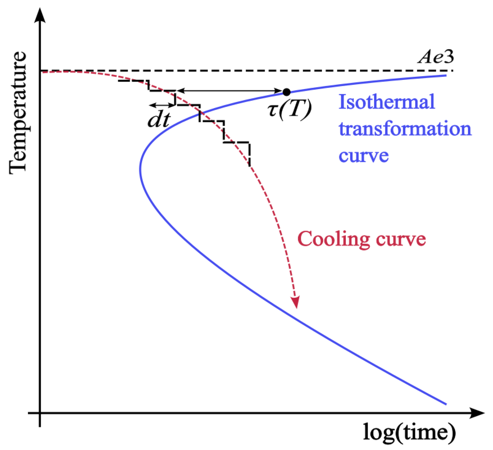
2.2. Converting to Non-Isothermal Behaviour
2.3. Predicting Constituent Behaviour
2.3.1. Predicting Ferrite
2.3.2. Predicting Pearlite
2.3.3. Predicting Bainite
2.4. Model Modifications
2.4.1. Modelling Carbon Partitioning
2.4.2. Adjusting Boundary Conditions
2.4.3. The Upper-to-Lower Bainite Transition
Predicting Ferrite Decarburisation
Predicting Cementite Formation Kinetics
Estimating
2.4.4. Predicting Martensite
2.5. Model Layout
2.5.1. Model Implementation
2.5.2. Model Assumptions
- Simple, homogeneous austenite grains—the basis of the model predicts steel cooling transformation behaviour within a single, homogeneous austenite grain of a set size. The rest of the material is assumed to comprise solely these homogeneous grains. As a consequence, constraints to constituent nucleation and growth due to the size and shape of the austenite grain, neighbouring grains and ongoing transformations within the grain are not explicitly considered, and any effect on transformation behaviour is assumed to be accounted for empirically. This also includes the impact of residual plastic strain as a result of specimen deformation. The partitioning of carbon is also assumed to occur homogeneously, and the remaining untransformed austenite is enriched equally.
- Additivity is satisfied—all transformations are assumed to be additive and a conversion to a ‘true’ TTT (before conversion to non-isothermal conditions) is deemed unnecessary.
- Consistent reaction rate—the time-dependent reaction rate of austenite decomposition is assumed to be consistent between each constituent, aside from martensite. This follows the original assumptions made in the Li model.
- Simplified transformations—austenite is assumed to only decompose into either ferrite (), pearlite ( + ), upper bainite (), lower bainite ( + intralath ) and martensite (’). Other transformations, such as second-phase particles or interlath carbides, are not currently considered. It is assumed that no constituent can transform simultaneously with another and transformations obey an order. Predictions for ferritic transformation behaviour are assumed to encompass the formation of all ferrite morphologies (allotriomorphic, Widmanstätten, and idiomorphic), as the predictions made by both Kirkaldy and Li do not distinguish between them. There is debate as to whether some of these morphologies should be considered ferritic; however, the determination of this lies outside the scope of this study.
- Diffusionless bainite transformation—there is much debate regarding the mechanism of the bainitic transformation and whether it is diffusion- or displacive controlled. For this model, for simplicity, it is assumed that bainite initially transforms displacively in the form of supersaturated laths of ferrite with carbon diffusion occurring after transformation.
3. Validation of Model
3.1. Experimental Measurements
3.2. Evaluating Modelled CCTs
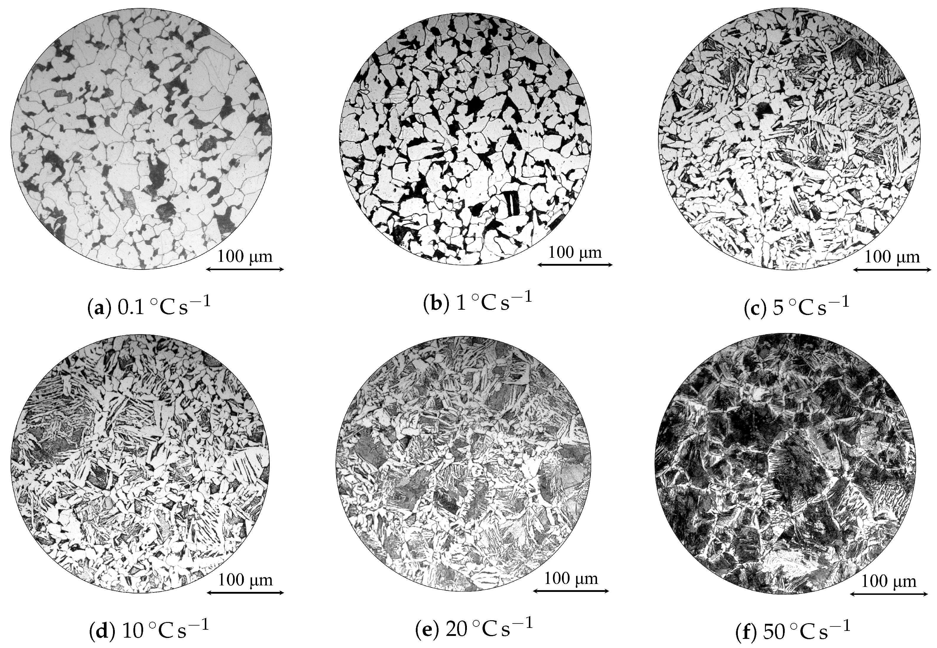
3.2.1. EN3B
3.2.2. EN8
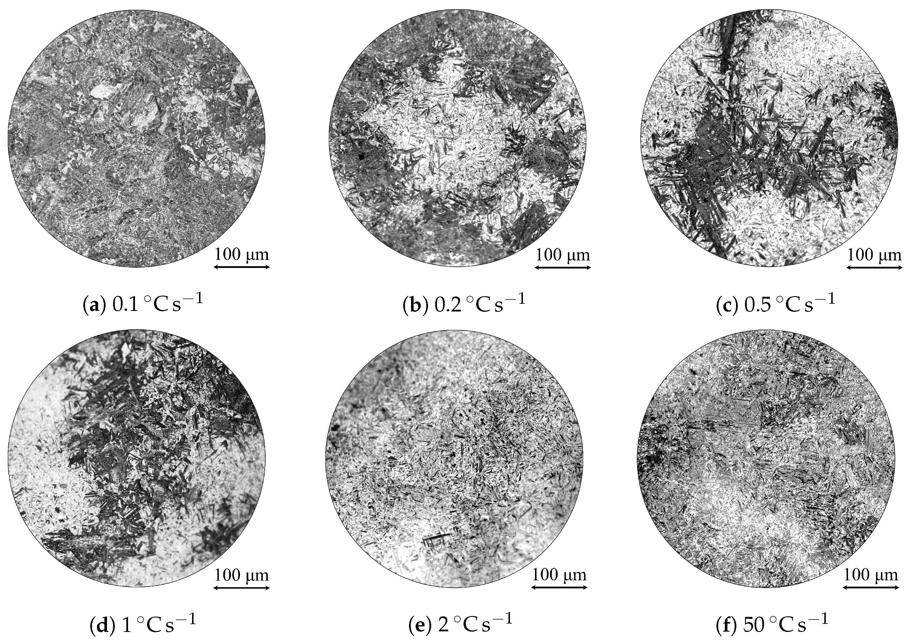
3.2.3. SA-540 B24
4. Discussion
4.1. Model Advantages
4.1.1. Improved CCT Predictions
4.1.2. Expanded Predictive Capabilities
4.1.3. Enhanced Usability and Accessibility
4.2. Model Limitations
4.2.1. Inherent Limitations
4.2.2. Over Partitioning
4.2.3. Material Heterogeneity
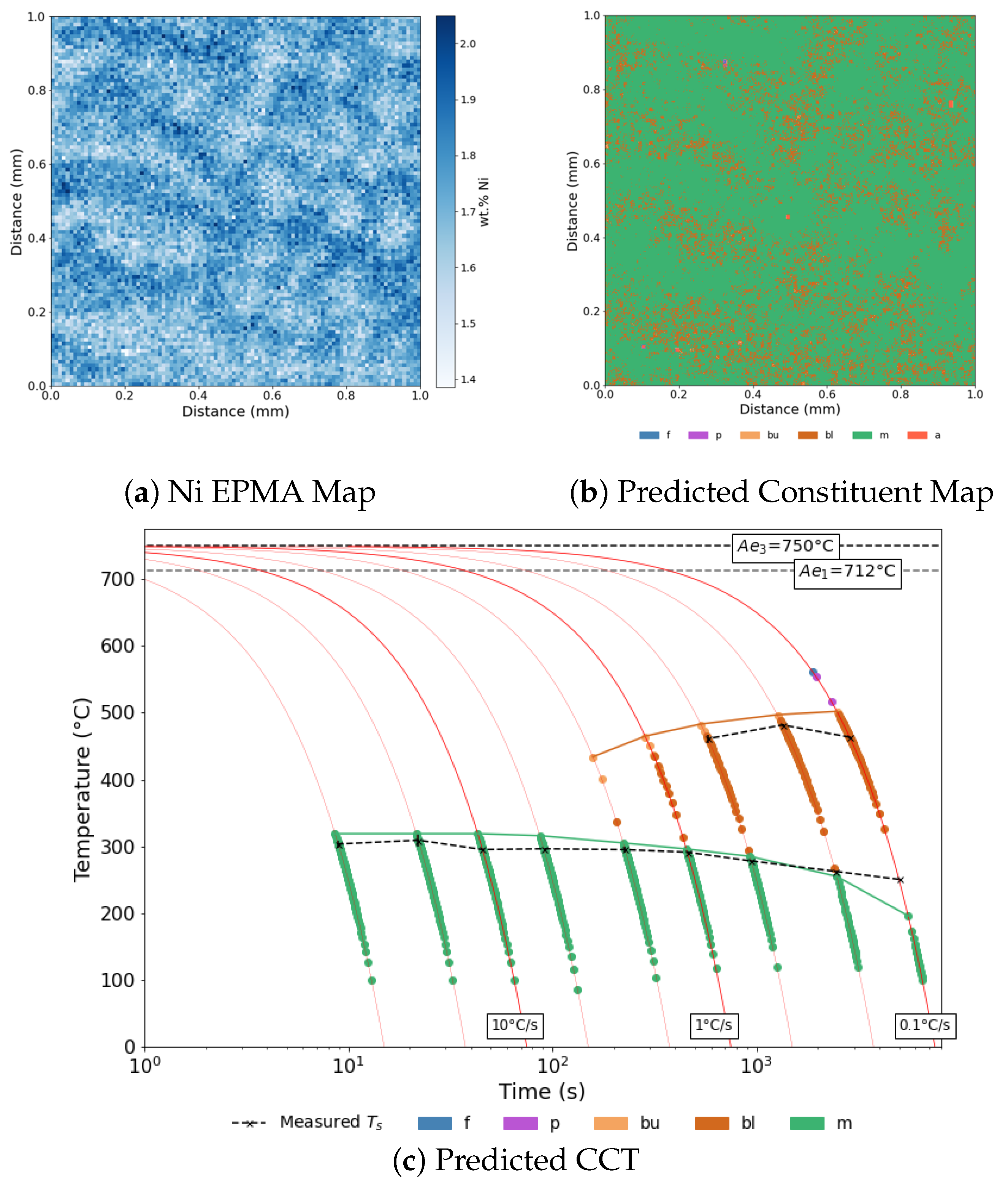
4.3. Considering Chemical Heterogeneity
5. Conclusions
- Li model predictions of continuous cooling behaviour were improved by the modifications outlined in this study. More accurate predictions were observed for all steels examined; however, this was best demonstrated in the SA-540 prediction, where the Li model underestimated the martensitic behaviour succeeding a higher-temperature bainitic transformation.
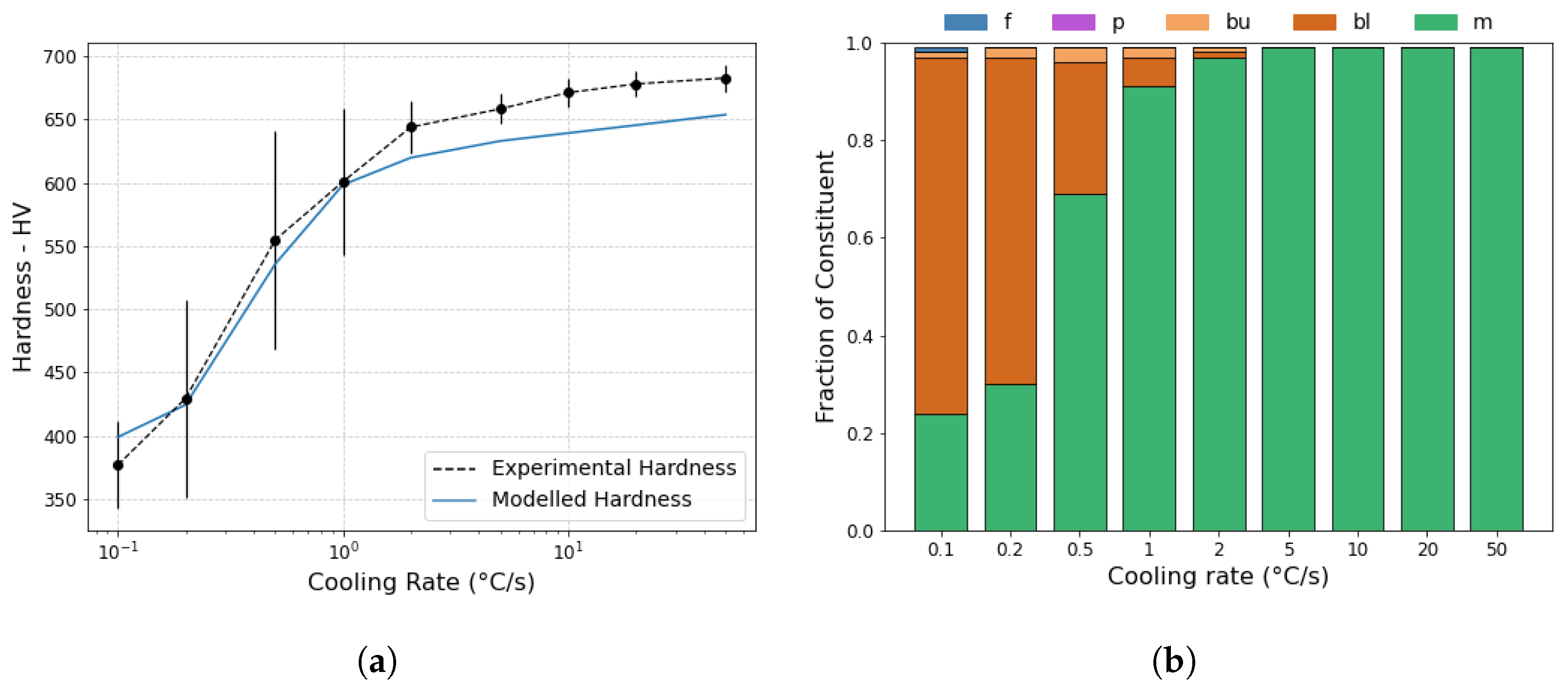
- The predictive capabilities of the model were expanded to include a prediction of final constituent fraction. The accuracy of these estimations were determined using hardness predictions, which agreed well with the experimental measurements.
- Although improvements were made to the CCT predictions, the accuracy of the proposed model is restricted by the inherent, empirical limitations of the original semi-empirical expressions. Correcting these limitations would require developing new sets of constituent transformation expressions around reliable and carefully controlled TTT and CCT datasets.
- The extent of carbon partitioning during austenite decomposition appears to be over-predicted, likely due to the technique used when measuring the empirical data, resulting in larger suppressions of . Nevertheless, the inclusion of this model incorporates a more realistic CCT prediction, but a more accurate measurement of partitioning would be required if this model was to be improved.
- Many disparities between the measured and predicted CCT behaviour were considered to be a result of microstructural heterogeneity within the examined material. The proposed model was implemented into a more sophisticated model that considered the measured chemical segregation in SA-540. Results from this adapted model showed an improved prediction of the SA-540 cooling behaviour.
Supplementary Materials
Author Contributions
Funding
Data Availability Statement
Conflicts of Interest
Appendix A. Deriving the Equation

| Function | a | b | Temperature Range |
|---|---|---|---|
| (J mol) | 7 | ||
| (J mol) | 650 | ||
| (J mol) | 0 | 0 |
| Alloying Element | (K per at.%) | (K per at.%) |
|---|---|---|
| Si | 0 | |
| Mn | ||
| Ni | ||
| Mo | ||
| Cr | ||
| V | ||
| Co | 19.5 | 16 |
| Al | 8 | 15 |
| Cu | 4.5 |
Appendix B. Calculating
| M | Mn | Si | Ni | Cr | Mo | Al |
|---|---|---|---|---|---|---|
| 0.0509 | 0.0 | 0.3031 | ||||
| 4.0507 | 7.7260 | 12.1266 |
Appendix C. Predicting Hardness
Appendix D. Chemical Compositional Ranges
| Eq. | C | Si | Mn | Ni | Cr | Mo | V | S | P | Ref. |
|---|---|---|---|---|---|---|---|---|---|---|
| / | 0.30–0.63 | 0.15–0.30 | 0.37–1.85 | 0.44–3.41 | 0.49–0.98 | 0.18–0.33 | [42] | |||
| 0.2–0.7 | 0.0–0.3 | 0.0–1.5 | 0.0–2.8 | 0.0–1.5 | 0.0–0.6 | [55] | ||||
| 0.09–0.55 | 0.11–1.74 | 0.20–1.67 | 0.15–5.04 | 0.07–3.34 | 0.0–1.0 | 0.01–0.20 | 0.004–0.043 | 0.005–0.038 | [61] |
Appendix E. EPMA Setup and Parameters
References
- Cias, W.W. Austenite Transformation Kinetics of Ferrous Alloys; Climax Molybdenum Company: Stowmarket, UK, 1978. [Google Scholar]
- Atkins, M. Atlas of Continuous Cooling Transformation Diagrams for Engineering Steels; Market Promotion Department, British Steel Corporation: London, UK, 1980. [Google Scholar]
- Vander Voort, G.F. Atlas of Time-Temperature Diagrams for Irons and Steels; ASM International: Russell Township, OH, USA, 1991. [Google Scholar]
- Scheil, E. Anlaufzeit der Austenitumwandlung. Arch. EisenhüTtenwes 1935, 8, 565–567. [Google Scholar] [CrossRef]
- Bhadeshia, H.K.D.H. Thermodynamic analysis of isothermal transformation diagrams. Met. Sci. 1982, 16, 159–165. [Google Scholar] [CrossRef]
- Ågren, J. Computer Simulations of Diffusional Reactions in Complex Steels. ISIJ Int. 1992, 32, 291–296. [Google Scholar] [CrossRef]
- Lee, J.L.; Bhadeshia, H.K.D.H. A methodology for the prediction of time-temperature-transformation diagrams. Mater. Sci. Eng. A 1993, A171, 223–230. [Google Scholar] [CrossRef]
- Lee, J.L.; Pan, Y.T.; Hsieh, K.C. Assessment of Ideal TTT Diagram in C-Mn Steel. Mater. Trans. JIM 1998, 39, 196–202. [Google Scholar] [CrossRef]
- van der Wolk, P.J.; Wang, J.; Sietsma, J.; van der Zwaag, S. Modelling the continuous cooling transformation diagram of engineering steels using neural networks Part I: Phase regions. Z. Metallkd. 2002, 93, 1199–1207. [Google Scholar] [CrossRef]
- Trzaska, J.; Dobrzański, L.A. Modelling of CCT diagrams for engineering and constructional steels. J. Mater. Process. Technol. 2007, 192–193, 504–510. [Google Scholar] [CrossRef]
- Geng, X.; Wang, H.; Xue, W.; Xiang, S.; Huang, H.; Meng, L.; Ma, G. Modeling of CCT diagrams for tool steels using different machine learning techniques. Comput. Mater. Sci. 2020, 171, 109235. [Google Scholar] [CrossRef]
- Minamoto, S.; Tsukamoto, S.; Kasuya, T.; Watanabe, M.; Demura, M. Prediction of continuous cooling transformation diagram for weld heat affected zone by machine learning. Sci. Technol. Adv. Mater. Methods 2022, 2, 402–415. [Google Scholar] [CrossRef]
- Kirkaldy, J.S.; Venugopalan, D. Prediction of Microstructure and Hardenability in Low Alloy Steels. In An International Conference on Phase Transformations in Ferrous Alloys; Marder, A.R., Goldstein, J.I., Eds.; Metallurgical Society of AIME: Philadelphia, PA, USA, 1984; pp. 125–148. [Google Scholar]
- Li, M.V.; Niebuhr, D.V.; Meekisho, L.L.; Atteridge, D.G. A Computational Model for the Prediction of Steel Hardenability. Metall. Mater. Trans. B 1998, 29B, 661–672. [Google Scholar] [CrossRef]
- Sente Software Ltd. JMatPro. 2023. Available online: https://www.sentesoftware.co.uk/jmatpro (accessed on 16 February 2023).
- Thermo-Calc Software. Thermo-Calc. 2023. Available online: https://thermocalc.com/ (accessed on 16 February 2023).
- Peet, M.; Bhadeshia, H.K.D.H. Program MAP STEEL MUCG83. 2020. Available online: https://www.phase-trans.msm.cam.ac.uk/map/steel/programs/mucg83.html (accessed on 16 February 2023).
- Lange, W.F.; Enomoto, M.; Aaronson, H.I. The Kinetics of Ferrite Nucleation at Austenite Grain Boundaries in Fe-C Alloys. Metall. Mater. Trans. A 1988, 19A, 427–440. [Google Scholar] [CrossRef]
- Yan, J.Y.; Ågren, J.; Jeppsson, J. Pearlite in Multicomponent Steels: Phenomenological Steady-State Modeling. Metall. Mater. Trans. A 2020, 51A, 1978–2001. [Google Scholar] [CrossRef]
- Leach, L.; Kolmskog, P.; Höglund, L.; Hillert, M.; Borgenstam, A. Critical Driving Forces for Formation of Bainite. Metall. Mater. Trans. A 2018, 49A, 4509–4520. [Google Scholar] [CrossRef]
- Leach, L.; Ågren, J.; Höglund, L.; Borgenstam, A. Diffusion-Controlled Lengthening Rates of Bainitic Ferrite a Part of the Steel Genome. Metall. Mater. Trans. A 2019, 50A, 2613–2618. [Google Scholar] [CrossRef]
- Stormvinter, A.; Borgenstam, A.; Ågren, J. Thermodynamically Based Prediction of the Martensite Start Temperature for Commercial Steels. Metall. Mater. Trans. A 2012, 43A, 3870–3879. [Google Scholar] [CrossRef]
- Hanumantharaju, A.K.G. Thermodynamic Modelling of Martensite Start Temperature in Commercial Steels. Master’s Thesis, KTH Royal Institute of Technology, Stockholm, Sweden, 2017. [Google Scholar]
- Huyan, F.; Hedström, P.; Höglund, L.; Borgenstam, A. A Thermodynamic-Based Model to Predict the Fraction of Martensite in Steels. Metall. Mater. Trans. A 2016, 47A, 4404–4410. [Google Scholar] [CrossRef]
- Saunders, N.; Guo, Z.; Li, X.; Miodownik, A.P.; Schillé, J.P. The Calculation of TTT and CCT Diagrams for General Steels. 2004. Available online: https://www.semanticscholar.org/paper/The-Calculation-of-TTT-and-CCT-diagrams-for-General-Saunders-Guo/28c913f0b561618d42bcb5ef08cf3ed449e16051 (accessed on 16 May 2023).
- Reséndiz-Flores, E.O.; Altamirano-Guerrero, G.; Costa, P.S.; Salas-Reyes, A.E.; Salinas-Rodríguez, A.; Goodwin, F. Optimal Design of Hot-Dip Galvanized DP Steels via Artificial Neural Networks and Multi-Objective Genetic Optimization. Metals 2021, 11, 578. [Google Scholar] [CrossRef]
- Krbat’a, M.; Eckert, M.; Cíger, R.; Kohutiar, M. Physical Modelling of CCT diagram of tool steel 1.2343. Procedia Struct. 2023, 43, 270–275. [Google Scholar]
- Zener, C. Kinetics of the Decomposition of Austenite. Trans. AIME 1946, 167, 550–595. [Google Scholar]
- Hillert, M. The Role of Interfacial Energy during Solid State Phase Transformations. Jernkont. Ann. 1957, 141, 758. [Google Scholar]
- Johnson, W.A.; Mehl, R.F. Reaction Kinetics in Processes of Nucleation and Growth. Trans. AIME 1939, 135, 416. [Google Scholar]
- Cahn, J.W. The Kinetics of Grain Boundary Nucleated Reactions. Acta Metall. 1956, 4, 449. [Google Scholar] [CrossRef]
- Guo, Z.; Saunders, N.; Miodownik, P.; Schillé, J.P. Modelling phase transformations and material properties critical to the prediction of distortion during the heat treatment of steels. Int. J. Microstruct. Mater. Prop. 2009, 4, 187–195. [Google Scholar] [CrossRef]
- Collins, J. Low Alloy Steel CCT Predictor. 2023. Available online: https://zenodo.org/record/7767620 (accessed on 19 June 2023).
- Hamelin, C.J.; Muránsky, O.; Smith, M.C.; Holden, T.M.; Luzin, V.; Bendeich, P.J.; Edwards, L. Validation of a numerical model used to predict phase distribution and residual stress in ferritic steel weldments. Acta Mater. 2014, 75, 1–19. [Google Scholar] [CrossRef]
- Sun, Y.L.; Vasileiou, A.N.; Pickering, E.J.; Collins, J.; Obasi, G.; Akrivos, V.; Smith, M.C. Impact of weld restraint on the development of distortion and stress during the electron beam welding of a low-alloy steel subject to solid state phase transformation. Int. J. Mech. Sci. 2021, 196. [Google Scholar] [CrossRef]
- Standard Test Methods for Determining Average Grain Size; ASTM International: West Conshohocken, PA, USA, 2010.
- Avrami, M. Kinetics of Phase Change I: General Theory. J. Chem. Phys. 1939, 7, 1103. [Google Scholar] [CrossRef]
- Cahn, J.W. Transformation Kinetics During Continuous Cooling. Acta Metall. 1956, 4, 572–575. [Google Scholar] [CrossRef]
- Umemoto, M.; Horiuchi, K.; Tamura, I. Transformation Kinetics of Bainite during Isothermal Holding and Continuous Cooling. Trans. ISIJ 1982, 22, 854–861. [Google Scholar] [CrossRef]
- Umemoto, M.; Horiuchi, K.; Tamura, I. Pearlite Transformation during Continuous Cooling and Its Relation to Isothermal Transformation. Trans. ISIJ 1983, 23, 690–695. [Google Scholar] [CrossRef]
- Wierszyłłowski, I.A. The Effect of the Thermal Path to Reach Isothermal Temperature on Transformation Kinetics. Metall. Trans. A 1991, 22A, 993–999. [Google Scholar] [CrossRef]
- Grange, R.A. Estimating Critical Ranges in Heat Treatment of Steels. Met. Prog. 1961, 79, 73–75. [Google Scholar]
- Andrews, K.W. Empirical formulae for the calculation of some transformation temperatures. J. Iron Steel Inst. 1965, 203, 721–727. [Google Scholar]
- Pickering, E.; Collins, J.; Stark, A.; Connor, L.D.; Kiely, A.A.; Stone, H.J. In situ observations of continuous cooling transformations in low alloy steels. Mater. Charact. 2020, 165, 1–10. [Google Scholar] [CrossRef]
- Bhadeshia, H.K.D.H.; Edmonds, D.V. The Mechanism of Bainite Formation in Steels. Acta Metall. 1980, 28, 1265–1273. [Google Scholar] [CrossRef]
- Bhadeshia, H.K.D.H.; Edmonds, D.V. The Bainite Transformation in a Silicon Steel. Metall. Trans. A 1979, 10A, 895–907. [Google Scholar] [CrossRef]
- Bhadeshia, H.K.D.H.; Edmonds, D.V. Bainite in silicon steels: New composition-property approach Part 1. Met. Sci. 1982, 17, 411–419. [Google Scholar] [CrossRef]
- Caballero, F.G.; Garcia-Mateo, C.; Santofimia, M.J.; Miller, M.K.; García de Andrès, C. New experimental evidence on the incomplete transformation phenomenon in steel. Acta Mater. 2009, 57, 8–17. [Google Scholar] [CrossRef]
- Bhadeshia, H.K.D.H. Bainite in Steels; Maney Publishing: Leeds, UK, 2015; Chapter 5; pp. 117–130. [Google Scholar]
- Sun, W.W.; Zurob, H.S.; Hutchinson, C.R. Coupled solute drag and transformation stasis during ferrite formation in Fe-C-Mn-Mo. Acta Mater. 2017, 139, 62–74. [Google Scholar] [CrossRef]
- Shiflet, G.J.; Bradley, J.R.; Aaronson, H.I. A Re-examination of the Thermodynamics of the Proeutectoid Ferrite Transformation in Fe-C Alloys. Metall. Trans. A 1978, 9A, 999–1008. [Google Scholar] [CrossRef]
- Bhadeshia, H.K.D.H. Driving force for martensitic transformation in steels. Met. Sci. 1981, 15, 175–177. [Google Scholar] [CrossRef]
- Bhadeshia, H.K.D.H.; Honeycombe, R. Steels: Microstructure and Properties; Butterworth-Heinemann: Oxford, UK, 2017; Chapter 15; pp. 421–455. [Google Scholar]
- Reynolds, W.T., Jr.; Li, F.Z.; Shui, C.K.; Aaronson, H.I. The Incomplete Transformation Phenomenon in Fe-C-Mo Alloys. Metall. Trans. A 1990, 21A, 1433–1463. [Google Scholar] [CrossRef]
- Lee, S.J.; Lee, Y.K. Thermodynamic Formula for the Acm Temperature of Low Alloy Steels. ISIJ Int. 2007, 47, 769–771. [Google Scholar] [CrossRef]
- Matas, S.J.; Hehemann, R.F. The Structure of Bainite in Hypoeutectoid Steels. Trans. AIME 1961, 221, 179–185. [Google Scholar]
- Pickering, F.B. The Structure and Properties of Bainite in Steels. In Transformation and Hardenability in Steels; Climax Molybdenum Company: Stowmarket, UK, 1967; pp. 109–129. [Google Scholar]
- Takahashi, M.; Bhadeshia, H.K.D.H. Model for transition from upper to lower bainite. Mater. Sci. Technol. 1990, 6, 592–603. [Google Scholar] [CrossRef]
- Guo, L.; Roelofs, H.; Lembke, M.I.; Bhadeshia, H.K.D.H. Modelling of transition from upper to lower bainite in multi-component system. Mater. Sci. Technol. 2016, 33, 430–437. [Google Scholar] [CrossRef]
- Speich, G.R. Tempering of Low-Carbon Martensite. Trans. Metall. Soc. AIME 1969, 245, 2553–2564. [Google Scholar]
- Steven, W.; Haynes, A.G. The Temperature of Formation of Martensite and Bainite in Low-alloy Steels. J. Iron Steel Inst. 1956, 123, 349–359. [Google Scholar]
- Kung, C.Y.; Rayment, J.J. An Examination of the Validity of Existing Empirical Formulae for the Calculation of Ms Temperature. Metall. Trans. A 1982, 13A, 328–331. [Google Scholar] [CrossRef]
- Koistinen, D.P.; Marburger, R.E. A general equation prescribing the extent of the austenite-martensite transformation in pure iron-carbon alloys and plain carbon steels. Acta Metall. 1959, 7, 59–60. [Google Scholar] [CrossRef]
- Yang, H.S.; Bhadeshia, H.K.D.H. Uncertainties in dilatometric determination of martensite start temperature. Mater. Sci. Technol. 2007, 23, 556–560. [Google Scholar] [CrossRef]
- Collins, J.; Dimosthenous, S.; Pickering, E.J. Steel Dilatometry Analysis. 2023. Available online: https://zenodo.org/record/7303893 (accessed on 19 June 2023).
- Instruments, O. AztecCrystal. 2023. Available online: https://nano.oxinst.com/azteccrystal (accessed on 22 February 2023).
- Blondeau, R.; Maynier, P.; Dollet, J.; Vieillard-Baron, B. Mathematical model for the calculation of mechanical properties of low-alloy steel metallurgical products: A few examples of its applications. In Heat Treatment ’76; Heat Treatment Committee of the Metals Society: London, UK, 1976; pp. 189–199. [Google Scholar]
- Penha, R.N.; Vatavuk, J.; Couto, A.A.; André de Lima Pereira, S.; Aragão de Sousa, S.; Canale, L.d.C.F. Effect of chemical banding on the local hardenability in AISI 4340 steel bar. Eng. Fail. Anal. 2015, 53, 59–68. [Google Scholar] [CrossRef]
- Taylor, M.; Fellowes, J.W.; Hill, P.O.; Rawson, M.J.; Burnett, T.L.; Pickering, E.J. The Effect of Compositional Heterogeneity on the Martensite Start Temperature of a High Strength Steel during Rapid Austenitisation and Cooling. IOP Conf. Mat. Sci. Eng. 2022, 1249, 012061. [Google Scholar] [CrossRef]
- Collins, J.; Piemonte, M.; Taylor, M.; Fellowes, J.; Pickering, E.J. Supplementary Material for “A Rapid, Open-Source CCT Predictor for Low Alloy Steels, and Its Application to Compositionally Heterogeneous Material”. 2023. Available online: https://zenodo.org/record/7770263 (accessed on 19 June 2023).
- Aaronson, H.I.; Domian, H.A.; Pound, G.M. Thermodynamics of the Austenite-Proeutectoid Ferrite Transformation. II, Fe-C-X Alloys. Trans. AIME 1966, 236, 768–781. [Google Scholar]
- Zener, C. Impact of Magnetism Upon Metallurgy. Trans. AIME 1955, 203, 619–630. [Google Scholar] [CrossRef]
- Siller, R.H.; McLellan, R.B. The Variation with Composition of the Diffusivity of Carbon in Austenite. Trans. Metall. Soc. AIME 1969, 245, 697–700. [Google Scholar]
- Siller, R.H.; McLellan, R.B. The Application of First Order Mixing Statistics to the Variation of the Diffusivity of Carbon in Austenite. Metall. Trans. 1970, 1, 985–998. [Google Scholar] [CrossRef]
- Bhadeshia, H.K.D.H. Diffusion of carbon in austenite. Met. Sci. 1981, 15, 477–479. [Google Scholar] [CrossRef]
- Krishtal, M.A. Diffusion Processes in Iron Alloys; Israel Program for Scientific Translations: Jerusalem, Israel, 1970; pp. 90–133. [Google Scholar]
- Wada, T.; Wada, H.; Elliott, J.F.; Chipman, J. Activity of Carbon and Solubility of Carbides in the FCC Fe-Mo-C, Fe-Cr-C, and Fe-V-C Alloys. Metall. Trans. 1972, 3, 2865–2872. [Google Scholar] [CrossRef]
- Rowan, O.K.; Sisson, R.D., Jr. Effect of Alloy Composition on Carburizing Performance of Steel. J. Phase Equilib. Diffus. 2009, 30, 235–241. [Google Scholar] [CrossRef]
- Babu, S.S.; Bhadeshia, H.K.D.H. Diffusion of carbon in substitutionally alloyed austenite. J. Mater. Sci. Lett. 1995, 14, 314–316. [Google Scholar] [CrossRef]
- Lee, S.J.; Matlock, D.K.; Van Tyne, C.J. An Empirical Model for Carbon Diffusion in Austenite Incorporating Alloying Element Effects. ISIJ Int. 2011, 51, 1903–1911. [Google Scholar] [CrossRef]


| Alloy | C | Si | Mn | Ni | Cr | Mo | S | Al | Cu | Fe |
|---|---|---|---|---|---|---|---|---|---|---|
| EN3B | 0.18 | 0.16 | 0.73 | 0.04 | 0.06 | 0.01 | 0.008 | 0.000 | 0.11 | Bal. |
| EN8 | 0.44 | 0.20 | 0.77 | 0.07 | 0.14 | 0.02 | 0.029 | 0.028 | 0.15 | Bal. |
| SA-540 | 0.40 | 0.26 | 0.75 | 1.81 | 0.86 | 0.32 | 0.008 | 0.031 | 0.08 | Bal. |
| Alloy | T (°C) | Step 1 | Step 2 | Step 3 |
|---|---|---|---|---|
| EN3B | 900 | Heat to T at 10 °C s. | Hold at T for 10 min. | Cool at 0.1, 0.2, 0.5, 1, 2, 5, 10, 20 or 50 °C s. |
| EN8 | 900 | Heat to T at 10 °C s. | Hold at T for 10 min. | Cool at 0.1, 0.2, 0.5, 1, 2, 5, 10, 20 or 50 °C s. |
| SA-540 | 870 | Heat to T at 10 °C s. | Hold at T for 2 h. | Cool at 0.1, 0.2, 0.5, 1, 2, 5, 10, 20 or 50 °C s. |
Disclaimer/Publisher’s Note: The statements, opinions and data contained in all publications are solely those of the individual author(s) and contributor(s) and not of MDPI and/or the editor(s). MDPI and/or the editor(s) disclaim responsibility for any injury to people or property resulting from any ideas, methods, instructions or products referred to in the content. |
© 2023 by the authors. Licensee MDPI, Basel, Switzerland. This article is an open access article distributed under the terms and conditions of the Creative Commons Attribution (CC BY) license (https://creativecommons.org/licenses/by/4.0/).
Share and Cite
Collins, J.; Piemonte, M.; Taylor, M.; Fellowes, J.; Pickering, E. A Rapid, Open-Source CCT Predictor for Low-Alloy Steels, and Its Application to Compositionally Heterogeneous Material. Metals 2023, 13, 1168. https://doi.org/10.3390/met13071168
Collins J, Piemonte M, Taylor M, Fellowes J, Pickering E. A Rapid, Open-Source CCT Predictor for Low-Alloy Steels, and Its Application to Compositionally Heterogeneous Material. Metals. 2023; 13(7):1168. https://doi.org/10.3390/met13071168
Chicago/Turabian StyleCollins, Joshua, Martina Piemonte, Mark Taylor, Jonathan Fellowes, and Ed Pickering. 2023. "A Rapid, Open-Source CCT Predictor for Low-Alloy Steels, and Its Application to Compositionally Heterogeneous Material" Metals 13, no. 7: 1168. https://doi.org/10.3390/met13071168
APA StyleCollins, J., Piemonte, M., Taylor, M., Fellowes, J., & Pickering, E. (2023). A Rapid, Open-Source CCT Predictor for Low-Alloy Steels, and Its Application to Compositionally Heterogeneous Material. Metals, 13(7), 1168. https://doi.org/10.3390/met13071168