Abstract
The accurate calibration of material parameters in crystal plasticity models is essential for applying crystal plasticity (CP) simulations. Identifying these parameters usually requires unfeasible single-crystal experiments or expensive time costs due to the use of traditional genetic algorithm (GA) optimization. This study proposed an efficient and interpretable method for calibrating the constitutive parameters with macroscopic mechanical tests. This approach utilized the Bayesian neural network (BNN)-based surrogate-assisted GA (SGA) optimization method to identify a group of constitutive parameters that can reproduce the experimental stress–strain curve and crystallographic orientation by crystal plasticity simulation. The proposed approach was performed on the calibration of typical high-entropy alloy material parameters in two different CP models. The use of the surrogate model reduces the call count of simulation in the parameter searching process and speeds up the calibration significantly. With the help of infill sampling, the accuracy of this optimization method is consistent with the CP simulation and not limited by the accuracy of the surrogate model. Another merit of this method is that the pattern that the BNN surrogate found in the model parameters can be interpreted with its integrated gradients, which helps us to understand the relationship between constitutive parameters and the output mechanical response. The interpretation of BNN can guide further experiment design to decouple particular parameters and add constraints provided by the attached experiment or prior knowledge.
1. Introduction
Under the impetus of digitalization and intellectualization tide of manufacturing, advanced simulation technology is required to accurately predict the manufacturing process and map the forming history to the product’s performance [1]. The crystal plasticity (CP) model utilizes the knowledge gained from experimental and theoretical studies of deformation physics of single crystals and polycrystals to predict anisotropic deformation behavior in a natural way. These models give insight into the evolution of crystallographic texture, dislocation density, stored mechanical energy, deformation-driven athermal transformations (e.g., twinning), etc.
The constitutive laws in the CP model, including the phenomenological model and the physics-based model, involve a set of adjustable parameters to provide the physics of the material behavior. The model accuracy strongly depends on the selected value of the adjustable material parameters. Therefore, the identification of material parameters is an essential prerequisite for the high predictive ability of the CP model. Theoretically, most of the constitutive parameters can be obtained from the mechanical response of a single crystal. However, these experiments are often unfeasible as typical engineering materials are often available as polycrystals, and a special method is required to probe into the mechanical behavior of single grains. One approach often used for polycrystals is a nanoindentation experiment. Another strategy involves the use of a coupled experimental–numerical procedure [2]. Since significant experimental effort is needed in these methods, identifying CP constitutive parameters via the inverse optimization methods from macroscopic stress–strain data determined by specific tensile or compression testing is generally preferred [3,4].
The procedure for the calibration of constitutive parameters with a macroscopic mechanical response is equivalent to solving the inverse problem of the CP model. The physic-based CP simulations, especially those of a full-field nature, often take minutes or hours to run [5]. Such optimization methods often require hundreds of simulations on different sets of parameters and take days or weeks to precisely calibrate the CP model. Thus, developing a computationally efficient and robust methodology to identify the constitutive parameters is significant for industry digitalization [6].
Many studies have employed gradient-based optimization methods for this purpose [4,7]. However, the main drawback of the gradient-based methods is that they are sensitive to the initial point, and the results are often inconsistent [8] since the constitutive laws are constructed with highly nonlinear equations, especially when encountering the micromechanics of complex engineering materials with multiple deformation mechanisms. Moreover, the gradient of the CP model is not always accessible. The reasons mentioned above limit the application of the gradient method in the parameter calibration of the CP model.
Another approach takes advantage of direct search methods, such as genetic algorithms (GAs) [9], searching the space by randomly generating solutions and providing new solutions based on the evaluation of the objective functions at the sampled points. As they negate the need for evaluating the gradient of the objective, direct search methods are able to optimize complex functions. These methods are capable of searching for the global optimum and do not have those drawbacks present in the gradient-based methods. However, these improvements come at the cost of computation efficiency [10].
The efficiency of GAs in CP parameter calibration is directly related to the call count of the CP simulation, which has the highest computational cost in fitness value calculation in the GA optimization process. Due to the expensive computational cost of numerical simulations using the CP model, it is rarely feasible to search a design space completely using simulation. The cost of the routine use of GAs can be cut down with the help of a surrogate model. So far, many studies have built surrogate models for the CP model to predict the physical response of a typical material, e.g., the texture evolution [11,12], dislocation density evolution [13], and stress distribution [14].
Data-based static models have been widely utilized to build the surrogate model for time-costing simulations in the optimization process [15,16]. In the research of Sedighiani et al. [6], a polynomial was fitted to approximate the constitutive response with the help of response surface methodology and using a GA to search the response surface in place of CP simulation. An artificial neural network (ANN)-based surrogate for CP simulation [17] is also a feasible approach to accelerating the process of GA searching. Data-based surrogate models, after training on a sufficient number of samples, can make an accurate prediction of the mechanical response much faster than their original counterpart. The surrogate-assisted GA (SGA) utilizes the surrogate model in fitness calculation and reduces the overall computational cost in the optimization procedure. Though some simulations are required to train the data-based surrogate model, the computational cost is still considered to be significantly lower than the cost of running the simulations required for GA searching.
However, the accuracy of the aforementioned surrogate-based method for CP parameter optimization is limited by the surrogate models. The optimization is completely based on the prediction of surrogate models after they are trained once on the initial samples provided by CP simulation. Additionally, this random initial sampling in the parameter space is redundant. It performs the same density of sampling at the promising point and around the optimum. In this study, a Bayesian neural network (BNN)-based surrogate is employed, and the infill sampling criteria (ISC) are utilized to allocate new sample points as well as to iteratively update the BNN surrogate during the optimization process. Moreover, the pattern learned by the BNN surrogate is further studied, providing insight into the calibration process thanks to the integrated gradients method. The remainder of this article is organized as follows. The next section details a BNN SGA with Expected Improvement (EI) as the ISC. In Section 3 and Section 4, we apply this methodology to calibrate the parameters of high-entropy alloys for phenomenological CP and a dislocation-density-based CP model with an experimentally determined mechanical response, based on which the impact of the ISC is discussed and the calibration result is analyzed with the information provided by the integrated gradients of the BNN surrogate.
2. Methodology
In this section, a novel approach is proposed to identify constitutive parameters of CP laws from macroscopic stress–strain curves using a BNN SGA. The construction of the BNN surrogate model is introduced, and the BNN SGA using EI as the infill sampling criteria in the acquisition process is detailed. The workflow of this method is presented in Figure 1. The experiment data are resampled and normalized to provide access to fitness for CP simulation and surrogate-predicted mechanical responses. The optimization started with a group of random initialized constitutive parameters, set as the initial population in the GA, which are optimized during iteration. After the surrogate model is trained on the data provided by CP simulation, the acquisition process is adopted to generate new solutions as well as assign a surrogate model for those solutions that are not expected to see improvement, and their fitness value is calculated with the surrogate model output in the next iteration. When the stop criteria of the optimization process are met, the best solution corresponding to the optimal constitutive parameters is output. The detailed optimization process of the BNN SGA is described in the following sections.
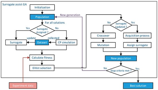
Figure 1.
Workflow of CP parameter calibration using SGA.
2.1. Optimization Algorithm
GA is a powerful optimization method that is able to search for the global optimum rather than getting stuck in local optimums [18], and is thus considered an alternative for optimization with a nonlinear objective function. It is based on a randomized search technique that imitates the principles of natural selection and evolution processes. In this study, a GA is employed to optimize the input CP parameters until the difference between the simulation-predicted mechanical response and experimentally determined response is minimized. PyGAD v2.16.0 (University of Ottawa, Ottawa, ON, Canada) [19], an open-source Python library for GAs, is utilized and modified to perform the multi-processing surrogate-assisted GA optimization in our implementation.
A GA consists of a series of different steps. As shown in Figure 2, the first generation is generated by uniform sampling during initialization, which provides training data for the first update of the surrogate model. In the selection process, the fitness value is calculated for each solution, based on which the parents are selected to produce the next generation. The genes in the offspring solutions are then modified with mutation and crossover operators. In this study, the mutation is implemented by randomly adding value to the genes, and the crossover operator swaps the genes of the parents after the crossover point. The selection, crossover, and mutation processes are iteratively performed on the new generation until the global optimum is found.
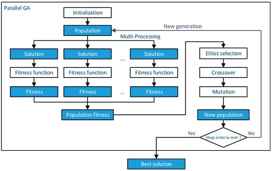
Figure 2.
Workflow of parallel GA.
The experimentally measured stress–strain curve is set as the target response, and an objective function is introduced based on the stress–strain curve. The root mean squared error (RMSE) is used to measure the difference between experimental and simulated results at the selected sample points, and is set as the objective function of the optimization:
where is the experimentally measured stress at the ith strain sample point, is the maximum value of the measured stress, is the predicted stress from the BNN surrogate or CP simulation for a group of constitutive parameters at the ith strain sample point, is the number of sample points, and denotes the relative difference between two curves under load condition l for the parameters. The reciprocal of the objective function is used to calculate the final fitness of solutions:
In elitist selection process, a few of the best solutions with the highest fitness are preserved and passed on to the next generation without modifying their genes. Elitist selection maintains the elite solutions and guarantees that achievement in fitness can be passed from generation to generation. The parameters for GA optimization are listed In Table 1.

Table 1.
The parameters for GA optimization.
The calculation of fitness can be implemented as parallel processing since the solutions are independent of each other during that process. However, in most GA applications, parallel processing does not reduce the computational cost compared to regular processing since multi-processing usually has a heavy computational cost. If the cost of assigning multi-processing is negligible compared to that of the fitness calculation, the overall run time can be significantly reduced by using multi-processing. In the context of CP model calibration, CP simulation always has a much higher computational cost than creating multi-processing. The calibration cost could then be slashed by using multi-processing.
2.2. BNN-Based Surrogate Model
Surrogate models work as a replacement for the expensive simulation in optimization. Previous studies suggested using an ANN and its variants to build the surrogate for the CP model [11,12]. Once sufficiently trained on the samples, the ANNs can obtain high accuracy in prediction, and this process runs very fast owing to the efficient matrix operation. Moreover, ANNs allow for incremental learning, and the model can be refined after being trained on new samples during optimization.
ANNs are proposed as a tool for classification and regression and do not provide uncertainty information around their predictions [20]. Since EI computation requires uncertainty information, coupling an ordinary ANN in the SGA method with EI as infill sampling criteria is not feasible. Meanwhile, the BNN could provide the posterior probability distribution over the weights [21], rather than the direct value of weights, and thus provides the uncertainty for EI calculation. Though using the traditional BNN is rarely feasible due to its expensive computational cost in training, this can be solved by using the MCDropout-based BNN.
The MCDropout method allows efficient BNN training by applying the Dropout technique in the training for the original ANN. Dropout is a regularization technique used in ANN training to reduce the flexibility of ANNs and prevent them from overfitting [22]. It is proven that adding dropout layers before the weight layer in a neural network is mathematically an approximation to the deep Gaussian process [20] i.e., the BNN. For the MCDropout-based BNN, the distribution of predicted parameters can be accessed with Monte Carlo (MC). estimation, i.e., performing stochastic forward propagation through the network for certain times and then calculating the average and variance of the prediction.
In this study, the MCDropout-based BNN is utilized as the surrogate model to predict the stress–strain curve for the input constitutive parameters. The BNN provides the distribution of the predicted objective value to calculate EI in the acquisition process. The neural network is first trained on the sample provided by CP simulation in the initial generation and then updated on the sample points with the highest EI and assigned to perform CP simulation in subsequent generations’ acquisition process.
2.2.1. Hyperparameters and Structure of BNN
The BNN utilized in this study consists of two parts, one from the input layer to output layer 1, and another from output layer 1 to output layer 2. The BNN is trained stepwise, instead of directly predicting the objective. It is trained to first predict the stress–strain curve in the form of feature parameters, and then to predict the objective from the curve features (Figure 3). This middle layer makes the output feature accessible for the surrogate model and allows for the extraction of BNN learned pattern. The first part, denoted as BNN1, is trained to capture the relationship between the stress–strain curve and the CP parameters, and works as the surrogate for CP simulation. The latter part, denoted as BNN2, predicts the objective distribution with the help of MCDropout. Both parts of the network have three dense layers, making them capable of capturing nonlinear relationships. The major hyperparameters and structure of the BNN are listed in Table 2.
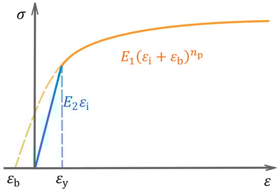
Figure 3.
Linear-elastic exponential-plastic model.
Table 2.
Hyperparameters and structure of BNN.
Activation functions transform the output of weight, typically nonlinearly, enabling the network to learn nonlinear functions. ReLU stands for the Rectified Linear Units, which is introduced in [23]. The dropout rate controls the percent of closed cells in the forward propagation. It should be mentioned that the BNN inputs (i.e., the CP parameters) have been normalized, and the output stress–strain curve is represented by a certain number of features. These transformations on the data extend the BNN to fit the data with different scales and units.
2.2.2. Data Processing
The activation for the output layer of BNN is the sigmoid function, which has a range of (0,1). Hence, the output must be rescaled or transformed to reproduce the physical quantities. Though there are no exact bounds for the input data, rescaling is performed on the input to speed up and stabilize the training process. If the BNN input vector has various scales in different dimensions, the gradient descent method for BNN training cannot effectively optimize the parameters in the BNN. In typical BNN applications, the data are normalized before training, or batch normalization (BN) [24] is added before the activation in the first layer.
In this study, input CP parameters were rescaled before being fed into the input layer, and the features of the stress–strain curve were extracted as the training target for output layer 1. The objective value was , which has already been normalized and can be directly set as the target for output layer 2. To normalize the CP parameters with different units, the CP parameters were rescaled into a range of (0, 1) using the min–max scaler:
where is the lth normalized CP parameter, is the ith original CP parameter, and are the manually estimated lower and upper bound for the ith CP parameter, respectively. The normalized CP parameter is utilized as the input for BNN1.
The stress–strain value () is a high-dimensional datum. It would be unfeasible for the BNN-based surrogate model to predict the stress at a massive number of sample points with a few input parameters. Simply reducing the number of sample points can lessen the difficulty of training the surrogate model, but it may fail to capture the features of the stress–strain curve. To overcome the “dimension curse”, the dimension of stress–strain curve data should be reduced before feeding it into the surrogate model. As shown in Figure 3, a prior model, the linear-elastic exponential-plastic model , is used to describe the stress–strain curve:
where is the ith stress and strain sample value, respectively, is the yield strain, is the bias for the exponential part, and is the exponent, is the variable controlling the value of yield stress, and is the elastic modulus. The parameter can be solved thanks to the continuity of the curve, and there are four independent feature parameters describing the stress–strain curve.
The feature parameters have different scales and cannot be directly fitted by the BNN. To enable the BNN to predict feature parameters, the stress–strain should first be normalized before fitting the linear-elastic exponential-plastic model:
where are the normalized values of , respectively, which have a range of (0, 1). are the maximum stress and strain value, respectively, of the experimental measured stress–strain curve. The normalized stress and strain values are used to calculate the normalized feature parameters of the linear-elastic exponential-plastic model .
where are the normalized curve features, whose range falls within (0, 1). These feature parameters can be calculated by the gradient method or stochastic optimization, e.g., difference evolution and the Newton-CG algorithm. The mean squared error is adopted as the objective for the four feature parameters in the linear-elastic exponential-plastic model to fit the stress–strain curve:
As shown by the calibration result in Section 4, the linear-elastic exponential-plastic model is flexible enough to fit a variety of stress–strain curves obtained from experiments and simulations with high accuracy. Moreover, the computational cost of fitting the linear-elastic exponential-plastic model is negligible compared to that of CP simulation.
The BNN1 is trained to correlate the parameter of the crystal plasticity model and these four featured parameters rather than the discrete stress–strain points. It reduces the stress–strain data from high-dimensional data (one sample point corresponds to one dimension) to several featured parameters ranging from 0 to 1. This is beneficial for the training of BNN. In addition, the analytical equation helps us to interpret the relationship between the mechanical response and parameters of the CP model by using integrated gradients. It gives specific meanings for the output of the BNN, which enables the interpretation of the calibration.
2.2.3. Implementation and Training of the Surrogate Model
The workflow of the BNN surrogate is presented in Figure 4. In the process of prediction, the first part of the BNN accepts normalized parameters as input and outputs the curve feature vector:
where is the input for BNN1, is the feature vector predicted by BNN1, equals to , the output of BNN1.
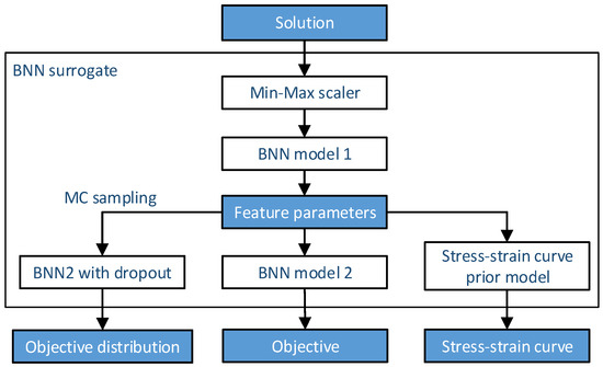
Figure 4.
Schematic diagram of BNN surrogate model.
The target feature parameters used for training BNN1 are calculated from the simulation output stress by optimizing feature parameters:
where is the normalized computational von Mises stress, and is the feature vector calculated from the simulation result.
For the second part of the BNN, the predicted feature parameters are accepted as input, and the RSME of the curve features defined in Equation (1) is set as the target output for BNN2. The BNN2 is trained with Dropout method, whose predict value and confidence is obtained by MC estimation.
where is the input for BNN2, is the objective predicted by BNN2, and is the standard deviation around the prediction. represent the expectation and variance estimation, respectively. The Monte Carlo sample number is set to 40 in this study.
The target objective for training BNN2 is calculated from the simulation output stress by:
The training samples and provided by simulation are used to train the BNN surrogate by minimizing the loss between and The mean square error (MSE) between the prediction and target value is chosen as the loss function for both BNN1 and BNN2,
where is the number of output features, and and are the BNN output and target value, respectively. The BNN cost for the current batch of training data is defined as the mean loss of all the samples:
where is the cost function, and is the size of the training batch. The BNN can be incrementally updated with a new batch of data. Incremental learning negates the need for repeated training of BNN on all the samples, significantly reducing the training time. Using a batch to represent all the samples and training on it could cause gradient instability. This problem can be reduced by tuning the batch size and training epochs.
Adaptive Moment Estimation (Adam) [25] is utilized to optimize the training parameters of the BNN. The training parameters are listed in Table 3.
Table 3.
The hyperparameters for BNN training.
Another data-based surrogate utilized in this study is the Lookup-based surrogate, which looks up for the similar input CP parameters from the simulated solutions’ dataset and directly returns their result. This strategy reduces the computational cost of calculating fitness on similar solutions. In GA searching, similar solutions can occur many times, especially when the population’s gene converges to the optimum. Thus, the utilization of the Lookup surrogate can effectively reduce the computational cost of the simulation for similar solutions. The threshold for adopting the Lookup surrogate is defined as follows:
where is the threshold for performing the Lookup surrogate model, and are the normalization of current candidate CP parameters and simulated CP parameters , respectively, denotes the distance between , and the -norm is used to measure the distance.
The Lookup surrogate is adopted when a group of parameters is firstly assigned to be simulated and the similar parameters group (i.e., the distance is less than ) has already been simulated. In this study, the is set to 0.001 and can be adjusted to a smaller value to obtain higher accuracy near the end of GA searching. It should be noted that the result of the Lookup surrogate will not be stored to train the BNN, since these samples have already been learned by the BNN.
2.3. MCDropout-Based BNN-Assisted GA
Many surrogate-based optimization methods have been utilized in recent studies to calibrate the CP parameters [6,17,26]. These surrogate models are only trained on initial samples, and optimization is performed based on the response of the surrogate model. In surrogate-based optimization, adjustable parameters would not converge to the global optimum if the surrogate model is built from only the initially sampled data or is simply an updated model with the current optimum as the new sample point [27]. This is because the surrogate model may not be sufficiently trained at the sample point in the optimization and is not accurate enough regarding its proximity to the global optimum. An iterative sampling refinement method is utilized to solve this problem, which allows the surrogate model to be updated on the new sample points generated during the optimization process. The criteria used to search the parameter space and refine the surrogate model with a promising sample point are the so-called infill sampling criteria [28]. Among various ISC, maximizing the EI is a widespread criterion and performs consistently well in the instances considered in the study compared with other ISC [29].
In this study, iterative sampling refinement is utilized so that the surrogate-assisted optimization can reaches the same accuracy as it could be achieved by directly minimizing the original objective function (i.e., using the CP simulation physical response to calculate the fitness value in a GA). Maximizing EI is chosen as the infill sampling criterion in the acquisition process, which generates a new population after the surrogate is trained [30]. In the acquisition process, the second part of the BNN is utilized to predict the objective distribution for the EI calculation.
2.3.1. Infill Sampling Criteria
The iterative sampling refinement method uses new sample points in promising regions to refine the surrogate model. The ISC are used to determine whether to sample the parameter space and refine the surrogate model or utilize the surrogate output, which is one of the key techniques in surrogate-based optimization. The EI for the candidate solution is given by:
where is the cumulative distribution function for the normal law and ϕ is its probability density function, is the best simulated cost found so far, is the predicted cost provided by the surrogate, and is the variance provided by the surrogate model for its predicted cost. In this study, the EI is calculated based on the BNN-predicted objective and its uncertainty according to Equations (11) and (12).
2.3.2. Acquisition Process
Once the surrogate is trained on the data provided by the initial generation, the acquisition process is activated. Figure 5 shows the workflow of the acquisition process. The acquisition process generates and selects sample points to perform CP simulation from the candidate solutions according to the ISC, and is employed as a trade-off between exploration and exploitation [31]. For the selected parent solutions with higher fitness values in the population, their offspring are generated by crossover and mutation. Then, the BNN surrogate is utilized to predict the objective with uncertainty information for all the offspring solutions. Their EI is computed by Equation (17). A proportion of children with the greater EI value are assigned to perform CP simulation. The remaining children who are less promising are set to be predicted by the surrogate model to gain speedup. In this study, the proportion assigned to the BNN surrogate model is set to different values, and its effect will be discussed.
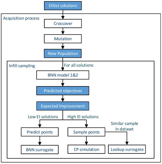
Figure 5.
Workflow of acquisition process and infill sampling.
3. CP Model and Set-Up of SGA
This section employs the proposed BNN SGA optimization method to calibrate the phenomenological CP model and dislocation-density-based CP model of a CoCrFeMnNi high-entropy alloy (HEA). For this HEA, a twelve-slip system of the {111} ⟨110⟩-type was considered, and the deformation twinning was omitted. The CP simulation toolkit DAMASK v3.0.0 alpha4 (Max-Planck-Institut für Eisenforschung GmbH, Düsseldorf, Germany) [32] was employed to perform the simulations. A cubic representative volume element (RVE) with 100 grains was used to reproduce the experimental result, as shown in Figure 6. The average grain size is about 6 μm, and uniaxial compression along the x-axis with a strain rate of 0.001 s−1 was applied. Python v3.8.10, NumPy v1.21.2, SciPy v1.7.1, and TensorFlow v2.8.0 (Google, Mountain View, CA, USA) were employed to construct the BNN SGA.
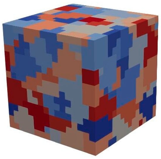
Figure 6.
The representative volume element (RVE) used for simulation.
3.1. CP Model for Calibration
3.1.1. Phenomenological CP Model
The applied phenomenological CP model, which was first proposed by Hutchinson for FCC crystals, is the most widely used phenomenological model [33]. The evolution of the shear rate () on each slip system is given by:
where , , and are the reference shear rate, resolve shear stress, and slip resistance of slip system α, respectively.
The slip resistance of slip system , , increasingly evolves from the initial value to a saturation value governed by the shear on slip and twin systems:
Here, are the hardening parameters. is the total number of slip systems. is the interaction coefficient between slip system , and is assumed to be 1.0 for coplanar slip systems and 1.4 for non-coplanar systems.
3.1.2. Dislocation-Density-Based CP Model
The dislocation-density-based CP model is the built-in model of DAMASK. A detailed description can be found in Ref. [32]. The shear rate is given by the Orown equation as
where is the Burgers vector length of slip families, is the initial glide velocity, is the activation energy of dislocation glide, is the Boltzmann constant, is the temperature, is the effective shear stress, and is the solid solution strength. and are the fitting parameters for glide velocity. The effective shear stress is computed as:
and the pass stress is given by:
where is the shear modulus, and are the slip–slip interaction matrices.
The evolution of dislocation densities is determined by dislocation multiplication, annihilation, and dipole formation. The evolution of dislocation density is given by:
where represents the mean free path (MFP) for dislocation, which governs the dislocation storage process. is the dislocation climb velocity and is given by:
where denotes the glide plane distance below which two dislocations form a stable dipole and denotes the glide plane distance below which two dislocations are annihilated. These are defined as:
where is a fitting parameter.
The MFP describes the pileup of dislocations in front of grain boundaries, dislocation–dislocation interaction, and the formation of twins, and is composed as:
where is the average grain size, is a fitting parameter, are projections for the forest dislocation density. Deformation twinning is omitted here since it infrequently occurred in this HEA.
3.2. Set-Up of SGA
3.2.1. Experiment Data
The experimental stress–strain response is obtained by a uniaxial compression at a strain rate of . The experimentally measured stress–strain curve is set as the target to be reproduced by a group of CP parameters. The initial orientation of the grains in the simulation is generated according to the orientation distribution of the texture. Figure 7 illustrates the pole figures characterizing the measured initial orientation and the sampled initial orientation used for CP simulation. As the initial orientations of the nodes within one grain are the same, the initial orientation distribution for CP simulation is very close to the experimental result. No evident texture was observed in the two pole figures, and the intensity of the initial orientation for CP simulation is slightly higher than that of the experimental one due to the smaller number of sampling grains of the RVE. The final orientation is utilized to validate the calibration result obtained from fitting the stress–strain curve. In this study, MTEX, the MATLAB toolbox for crystallographic textures analysis, is employed to process the EBSD data and draw the pole figures for material textures.
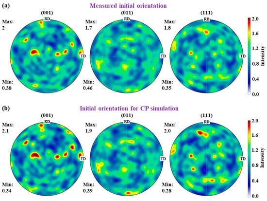
Figure 7.
Pole figure characterizing (a) the measured initial orientation and (b) the initial orientation for CP simulation.
3.2.2. Input Parameters for SGA
The elastic constants , , , reference shear rate , and the magnitude of the Burgers vector were regarded as the definitive constitutive parameters for CP simulation, as listed in Table 4. Parameters and in the dislocation-density-based CP model can be set to 1.0 for cuboidal shapes of local obstacles [34]. All the simulations were conducted at room temperature, and the temperature T was thus set as 300 K. The adjustable material parameters of the phenomenological and dislocation-density-based CP model and their reference ranges, which need to be optimized to reproduce the experimental stress–strain curves and pole figures, are listed in Table 5 and Table 6, respectively.
Table 4.
Definitive constitutive parameters for the phenomenological CP model.
Table 5.
Ranges of the adjustable parameters for the phenomenological CP model.
Table 6.
Ranges of the adjustable parameters for the dislocation-density-based CP model.
3.2.3. Hyperparameters for SGA
Table 7 lists the hyperparameters for surrogate-assisted searching that control the use of Lookup and BNN surrogates. The proportion of the performing BNN surrogate is set to 0.2, 0.4, 0.6, and 0.8 in different runs, the results of which are compared and discussed in Section 4.
Table 7.
Hyperparameters for SGA.
4. Results and Discussion
4.1. Optimization Process
According to the input parameters and the SGA hyperparameters listed in Table 4, Table 5, Table 6 and Table 7, four SGA searches are performed with different values. In this section, we take the phenomenological CP model as an example, and the influence of on optimization and the speedup provided by the SGA are discussed by analyzing the data extracted from their optimization processes.
4.1.1. Influence of
Figure 8 shows the best fitness in each generation calculated by phenomenological CP simulation and BNN surrogate model under various . As shown in Figure 8, affects the fitness improvement of the solutions assigned to CP simulation. With the increase in , the best fitness values calculated by the BNN surrogate and CP simulation tended to mix with each other, implying a worse performance of the acquisition process. This can be explained by two related aspects. Firstly, the BNN surrogate relies on the samples provided by CP simulation to be incrementally trained, improving its accuracy. On the other hand, the ISC rely on the BNN’s accuracy to provide more confidence in assigning CP simulation to those solutions that are expected to gain higher fitness. A higher value leads to a lack of training data for the BNN surrogate and a lack of confidence in the ISC for model assignment in the acquisition process and thus the failure to allocate promising sample points. A lower value guarantees the BNN surrogate’s accuracy and the stability of the acquisition process, while losing the speedup provided by using the surrogate model. To settle this contradiction, we defined a cumulative fitness improvement (CFI) per CP simulation to measure the effectiveness of the SGA process:
where is the best fitness found till generation , denotes the number of CP simulations performed in generation , and n is the current generation number.
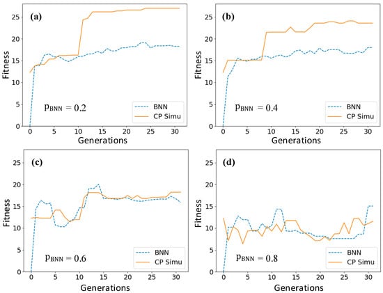
Figure 8.
The best fitness in each generation calculated by phenomenological CP simulation and BNN when equals (a) 0.2, (b) 0.4, (c) 0.6, and (d) 0.8.
CFI generally describes the fitness improvement contributed by each CP simulation during the SGA optimization process. The CFI in different SGA runs for the phenomenological CP model under different is presented in Figure 9, where the case shows a consistently higher CFI. The CFI progressively increases when , indicating a stable searching process but with more computational cost. When , the CFI is slowly increasing with fluctuations, indicating the acquisition process started to lose efficacy. It is worth noting that when , due to the interference of the surrogate model, the SGA search has not made progress in fitness improvement, resulting in a negative value. According to the discussion above, is considered the best value for obtaining a balance between the optimization speedup and the fitness maximization.
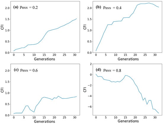
Figure 9.
The cumulative fitness improvement in different SGA runs when equals (a) 0.2, (b) 0.4, (c) 0.6, and (d) 0.8.
4.1.2. The Speedup Provided by Parallel SGA
Two SGA optimization processes with and are considered in this section, and the number of parallel processes in GA fitness calculation is set as 12. Assuming that the cost of running the surrogate model is negligible compared to the CP simulation and the computing time for different CP simulations are similar, the computational time cost ratio of the SGA to the original GA is equivalent to the call count ratio. The number of surrogate (the BNN and the Lookup surrogate model) calls and phenomenological CP simulation calls needed to calculate the fitness in each generation is presented in Figure 10. Consequently, the speedup provided by the SGA method can be estimated with the cumulation of the call counts using the following equation:
where is the speedup achieved using parallel SGA compared to traditional parallel GA optimization, and are the expected time cost of running the SGA and GA, respectively, and are the number of CP simulation and surrogate calls in generation i, respectively, and is the current generation. Around the end of the optimization process, when the genes in the population converge to the optimum and become similar to each other, the number of Lookup surrogate calls increases, providing more speedup than could be achieved by only utilizing the BNN surrogate. The speedup of the optimization process under the considered are 2.917 (Figure 10a) and 3.765 (Figure 10b), respectively, compared to the ordinary parallel GA. When considering the speedup provided by parallel fitness calculation, using the parallel surrogate-assisted GA eventually led to a speedup of around 50 compared to the serial GA on the workstation used in this study.
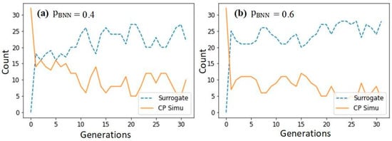
Figure 10.
The number of phenomenological CP simulation calls and surrogate (the BNN or Lookup) calls in GA generations (a) , (b) .
4.2. Calibration Results and Interpretation
In this section, 2 separate SGA searching processes are run for 32 generations using the numerical input mentioned in Section 3 with being equal to 0.4.
4.2.1. Comparison of Experimental and Simulated Results
The adjustable parameters of the best solution in two runs of the phenomenological and dislocation-density-based CP models are listed in Table 8 and Table 9, respectively. The mechanical response and pole figures are compared in Figure 11. For both CP models, the SGA-output best solution in the two runs showed good agreement between CP simulation prediction and the experimentally measured stress–strain curve. The error between the target curve and two simulation runs quantified by the distances defined by Equation (1) is 4.18% and 4.15% for the phenomenological CP model and 2.04% and 1.80% for the dislocation-density-based CP model, respectively. Despite the good fit of the stress–strain curve in optimization, there is a relatively large difference in the optimized constitutive parameter , and especially for . In run 1, parameter of the best solution lies in the range [100, 700] MPa, while in run 2, it reaches the upper bound, while for the dislocation-density-based CP model, the parameters show a similar convergence tendency but different converge values in two runs. These two different sets of parameters result in almost the same mechanical response. Parameters and show a large distribution range in two runs, while converge to a single point. The dislocation-density-based CP model involves more parameters to characterize the mechanical response of materials than the phenomenological model, showing fewer constraints of the stress–strain curve data and more uncertainty in the calibration results. This difference in results from different runs is further discussed in Section 4.2.3, with the interpretation of the BNN.
Table 8.
The optimal parameters of the phenomenological CP model.
Table 9.
The optimal parameters of the dislocation-density-based CP model.
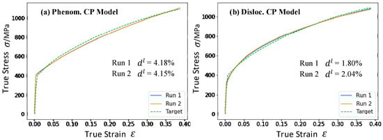
Figure 11.
The stress–strain curve of best solution calculated by CP simulation in two runs (run 1, run 2), and the experiment stress–strain curve (target) in (a) a phenomenological CP model and (b) dislocation-density-based CP model. , as defined in Equation (1), denotes the relative difference between simulation-calculated stress–strain curve and experiment stress–strain curve in two runs.
Figure 12 shows the comparison of experimental and simulated pole figures using different CP models. Both the pole figures obtained by the phenomenological and dislocation-density-based CP models successfully reproduced the (011) fiber texture observed in the measured one (Figure 12a). The orientation distribution and maximum value of texture intensity agree well with the experimental counterpart.
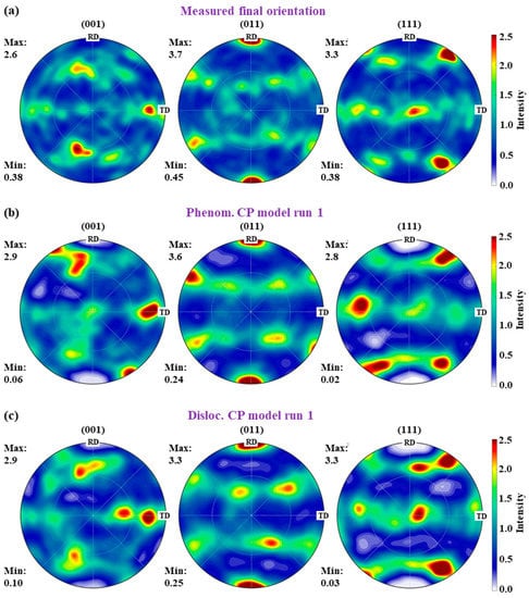
Figure 12.
Pole figure of (a) measured final orientation, (b) phenomenological CP model run 1, and (c) dislocation-density-based CP model run 1.
4.2.2. The Gene Evolution
Figure 13 shows the evolution of the gene corresponding to and in the phenomenological CP model and and in the dislocation-density-based CP model. When the searching process stopped at generation 32, the solutions’ gene gathered around the same value, suggesting that the global optimum had been found. It should be mentioned that the incremental mutation operator is employed in the GA, which randomly increases or decreases the value of genes in the mutation process. This method is conducive to exploring the parameter space near the optimal solution and simultaneously improving the performance of BNN prediction near the optimum. The fine-tuning of the mutation, with one parameter fixed and another changing, resulted in the cross-like sampling point around the optimum.
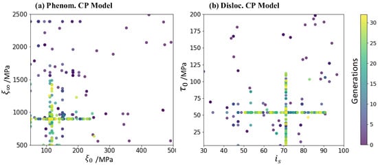
Figure 13.
The evolution of the gene corresponding to (a) and in the phenomenological CP model and (b) and in the dislocation-density-based CP model.
This evolution of sample points also indicates the adaptive nature of infill sampling and requires fewer samples to reach the same accuracy around the optimum than the uniform random sampling method in other CP parameters calibration studies. The regions that are not expected to cover the optimum are sparsely sampled, while the interested region is sufficiently probed to make an accurate prediction.
Figure 14 shows the candidate solutions’ parameter distribution in the last generation in the two runs of different CP models. It can be observed that the converge value of parameter and of the phenomenological CP model is consistent in run 1 and run 2, while shows a wide range of distribution in these solutions and converges to a different point, as shown in Figure 14a,b. For the dislocation-density-based CP model (Figure 14c,d), the optimized parameters in run 1 and run 2 are significantly different. This is caused by two reasons. One is that some parameters have little impact on the mechanical response, and the other is the coupling effects between different CP parameters. This parameter uncertainty is severer in the complex CP model with many parameters to be determined. These effects will be further discussed in Section 4.2.3.
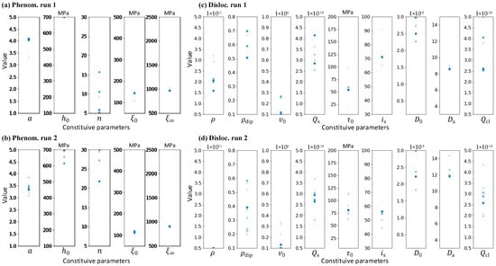
Figure 14.
The parameter distribution of the candidate solutions in the last generation in (a) phenomenological model run 1, (b) phenomenological model run 2, (c) dislocation density model run 1, and (d) dislocation density model run 2. The semitransparent blue points represent the certain constitutive parameters of solutions in the last generation, overlap points will show deeper color.
4.2.3. Interpretation by BNN-Integrated Gradients
In this study, the BNN surrogate is not trained to predict the objective directly but first learns to predict stress–strain curve features and then predicts the objective, which provides interpretability for the BNN surrogate model. The integrated gradients [37] are used to analyze the surrogate model, providing insight into the relationship between CP parameters and the stress–strain curve. The integrated gradients can be approximated via the summation of gradients at small intervals along the path from the baseline to the input x:
where is the approximation of integrated gradients for input parameter , and m is the number of steps in the Riemman approximation of the integral. In this study, m is set to 50, and the baseline is set as 0, which corresponds to the lower bound of the input material parameters. It should be noted that, in this study, the BNN’s gradients are sampled in a manner wherein all the parameters increase simultaneously to show the input parameters’ global impact on the feature parameters.
The stress–strain curve shown in Figure 3 is represented as four feature parameters in a normalized form defined in Section 2.2.2 and utilized as the BNN1 output. Figure 15 shows the integrated gradients of the input parameters of the phenomenological CP model to the output feature parameters. is the most sensitive feature, and controls the curvature of the plasticity part. A larger or smaller produces a stress–strain curve with a more obvious exponential increase in the plasticity part, corresponding to a larger value. Parameters and have a positive contribution to and a negative contribution to ; thus, increasing and will result in a stress–strain curve with a lower yield point and higher saturation stress. is indirectly affected by yield and saturate stress, which is shown to be the least sensitive feature in the curve.
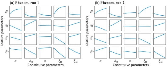
Figure 15.
The integrated gradients for the BNN surrogate of the phenomenological CP model in (a) run 1 and (b) run 2.
In both run 1 and run 2, the constitutive parameter shows a slight influence on all the feature parameters, and a varying may not influence the output. This causes difficulty in accurately calibrating parameter and accordingly shows a wide range of candidate values (Figure 14). This accounts for the large difference in parameter observed in the results of two runs (Table 8). There also exists a relatively large difference in parameters and in the two runs, which is the result of parameter coupling. In Figure 15, the parameters and show an opposite effect on the stress–strain curve features, indicating that these parameters can increase or decrease simultaneously while obtaining almost the same output features. It should be noted that the parameter , which controls the yield strain, does not contribute much to the fitness calculation; thus, the different effect on found in run 1 and run 2 is neglectable in parameter coupling. It can be seen that the effect of is somewhat similar to that of , indicating a potential coupling between . Thus, when is limited by the upper bound, may act as its substitution, resulting in a slightly larger value of (Table 8, run 2). Parameter shows good consistency in two runs, indicating that it was easily determined by the optimization process.
Figure 16 presents the integrated gradients for the BNN surrogate of the dislocation-density-based CP model. The parameters show more complex coupling between parameters in this calibration compared with the simple two-parameter coupling in the phenomenological CP model. and are the most influential parameters on the output features; thus, by fitting the stress–strain curve, they show good convergence (Figure 14). However, due to potential coupling with the other parameters, their converge points are influenced. is a relatively influential parameter and is constrained within a range. and show various effects in different runs. When it shows a greater impact on the feature parameters (characterizing the mechanical response), as seen in Figure 16, its distribution correspondingly has a narrow range, as seen in Figure 14. This results from the different influences of these parameters on different sample regions. The BNN captures this pattern and can successfully explain the distribution of the candidate solution’s parameters.
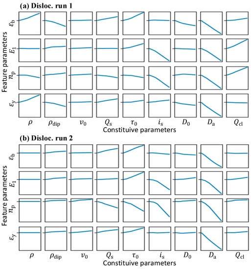
Figure 16.
The integrated gradients for the BNN surrogate of dislocation-density-based CP model in (a) run 1 and (b) run 2.
Though most of the CP parameters cannot be exactly determined by fitting the stress–strain curve and showing coupling or noneffective tendency, they are constrained to a certain extent. The interpretation of the BNN can guide further experiment design to decouple particular parameters and add constraints provided by the attached experiment or prior knowledge. With the knowledge extracted from the BNN, the constraint of the macroscopic mechanical response on the model parameters is outlined, and this can be used to guide future experiment design. In general, a parameter is well constrained by the fitting data and converges to a consistent point when it (a) shows a significant impact on the output features and (b) does not couple with other adjustable parameters. The parameters showing a range distribution in the last generation of the SGA are considered only partly constrained in a range with the experiment data, with a slighter influence on the output features. Though a lack of constraints exists, some parameters can be determined with a macroscope mechanical response, and others need further constraints (e.g., additional experiment dataset as the fitting target or prior knowledge-based constraints for the GA) or decoupling (e.g., calibrate coupled parameters separately) to be further calibrated.
5. Conclusions
We aimed to accelerate the calibration of a CP model and maintain its accuracy simultaneously. A BNN-based surrogate was employed, and the infill sampling(IS) method were utilized to allocate new sample points as well as iteratively update the BNN surrogate during the optimization process. By using the integrated gradients, the evolution of parameters during the calibration process and the coupling effect of different parameters were analyzed. The main conclusions can be drawn as follows:
- A BNN SGA optimization method was proposed for calibrating crystal plasticity models. The MCDropout-based BNN makes a prediction with uncertainty information, and guides the GA optimization process by infill sampling. The BNN is trained stepwise to predict feature parameters of the mechanical response and provides interpretability for the surrogate.
- Maximizing EI is used as the infill sampling criteria, determining which candidate solutions should be selected as new sample points and performing the time-consuming simulation. The Lookup-based surrogate, which queries the dataset and directly returns the fitness for similar solutions, is another data-based surrogate utilized in this study.
- The BNN SGA method is applied to the typical phenomenological and dislocation-density-based CP models of an HEA. The speedup of the optimization process is 2.917 and 3.765 when the proportion of performing BNN surrogates equals 0.4 and 0.6, respectively. Using the identified parameters, the stress–strain curve and pole figure obtained by compression tests were successfully reproduced by CP simulation.
- This method allows for interpretation of the BNN surrogate using the integrated gradients and extract information of the relationship between input CP parameters and the feature of the mechanical response. The effect of the CP parameters on the stress–strain curve and the coupling between CP parameters was analyzed. The interpretation of the BNN can guide further experiment design to constrain or decouple particular CP parameters to refine the calibration result.
- The SGA method proposed in this paper can be extended to calibrate CP models including more complex deformation mechanisms, such as deformation twinning and phase transformation. The BNN surrogate with iterative infill sampling and integrated gradients can also be extended to establish an interpretable and fast multiscale surrogate plasticity model that characterizes the microscale slip, mesoscale strain, and macroscale mechanical response.
- Like most optimization algorithms, this method relies on an initial parameter range. Due to the complex nonlinear relationship between parameters of the CP model, the range of other parameters will change dramatically if the range of one parameter is modified, so it is not easy to determine the initial range. In this paper, the coupling between CP parameters and the effect of CP parameters on the mechanical response are demonstrated by means of an integral gradient, but no quantitative model is introduced to systematically describe their coupling relationship. There is no quantitative description of how the provided experimental data constrain the results of the calibration. Future research could focus on breaking these limitations and propose a more robust calibration method.
Author Contributions
Methodology, software, investigation, visualization, writing—original draft preparation, S.Y.; conceptualization, funding acquisition, visualization, writing—review and editing, X.T.; data curation, validation, writing—review and editing, L.D., P.G., M.Z. and J.J.; project administration, funding acquisition, X.W. All authors have read and agreed to the published version of the manuscript.
Funding
This research was funded by the National Natural Science Foundation of China (No. 52090043), the Aeronautical Science Foundation of China (No. 20200036079001), and the National Natural Science Foundation of China (No. 52105337).
Data Availability Statement
Not applicable.
Conflicts of Interest
The authors declare no conflict of interest.
References
- Tang, X.; Wang, Z.; Deng, L.; Wang, X.; Long, J.; Jiang, X.; Jin, J.; Xia, J. A Review of the Intelligent Optimization and Decision in Plastic Forming. Materials 2022, 15, 7019. [Google Scholar] [CrossRef] [PubMed]
- Bertin, M.; Du, C.; Hoefnagels, J.P.M.; Hild, F. Crystal plasticity parameter identification with 3D measurements and Integrated Digital Image Correlation. Acta Mater. 2016, 116, 321–331. [Google Scholar] [CrossRef]
- Do, B.; Ohsaki, M. Bayesian optimization for inverse identification of cyclic constitutive law of structural steels from cyclic structural tests. Structures 2022, 38, 1079–1097. [Google Scholar] [CrossRef]
- Herrera-Solaz, V.; LLorca, J.; Dogan, E.; Karaman, I.; Segurado, J. An inverse optimization strategy to determine single crystal mechanical behavior from polycrystal tests: Application to AZ31 Mg alloy. Int. J. Plast. 2014, 57, 1–15. [Google Scholar] [CrossRef]
- Savage, D.J.; Feng, Z.; Knezevic, M. Identification of crystal plasticity model parameters by multi-objective optimization integrating microstructural evolution and mechanical data. Comput. Methods Appl. Mech. Eng. 2021, 379, 113747. [Google Scholar] [CrossRef]
- Sedighiani, K.; Diehl, M.; Traka, K.; Roters, F.; Sietsma, J.; Raabe, D. An efficient and robust approach to determine material parameters of crystal plasticity constitutive laws from macro-scale stress-strain curves. Int. J. Plast. 2020, 134, 102779. [Google Scholar] [CrossRef]
- Saleeb, A.F.; Gendy, A.S.; Wilt, T.E. Parameter-Estimation Algorithms for Characterizing a Class of Isotropic and Anisotropic Viscoplastic Material Models. Mech. Time-Depend. Mater. 2002, 6, 323–361. [Google Scholar] [CrossRef]
- Andrade-Campos, A.; Thuillier, S.; Pilvin, P.; Teixeira-Dias, F. On the determination of material parameters for internal variable thermoelastic¨Cviscoplastic constitutive models. Int. J. Plast. 2007, 23, 1349–1379. [Google Scholar] [CrossRef]
- Deb, K.; Pratap, A.; Agarwal, S.; Meyarivan, T. A fast and elitist multiobjective genetic algorithm: NSGA-II. IEEE Trans. Evol. Comput. 2002, 6, 182–197. [Google Scholar] [CrossRef]
- Furukawa, T.; Sugata, T.; Yoshimura, S.; Hoffman, M. An automated system for simulation and parameter identification of inelastic constitutive models. Comput. Methods Appl. Mech. Eng. 2002, 191, 2235–2260. [Google Scholar] [CrossRef]
- Pandey, A.; Pokharel, R. Machine learning enabled surrogate crystal plasticity model for spatially resolved 3D orientation evolution under uniaxial tension. arXiv 2020, arXiv:200500951. [Google Scholar]
- Pandey, A.; Pokharel, R. Machine learning based surrogate modeling approach for mapping crystal deformation in three dimensions. Scr. Mater. 2021, 193, 1–5. [Google Scholar] [CrossRef]
- Yang, Z.; Papanikolaou, S.; Reid, A.C.E.; Liao, W.-K.; Choudhary, A.N.; Campbell, C.; Agrawal, A. Learning to Predict Crystal Plasticity at the Nanoscale: Deep Residual Networks and Size Effects in Uniaxial Compression Discrete Dislocation Simulations. Sci. Rep. 2020, 10, 8262. [Google Scholar] [CrossRef]
- Rezaei Mianroodi, J.; Siboni, N.H.; Raabe, D. Teaching Solid Mechanics to Artificial Intelligence: A fast solver for heterogeneous solids. arXiv 2021, arXiv:210309147. [Google Scholar]
- Forrester, A.I.J.; Keane, A.J. Recent advances in surrogate-based optimization. Prog. Aerosp. Sci. 2009, 45, 50–79. [Google Scholar] [CrossRef]
- Williams, B.A.; Cremaschi, S. Surrogate model selection for design space approximation and surrogatebased optimization. Comput. Aided Chem. Eng. 2019, 47, 353–358. [Google Scholar]
- Ibragimova, O.; Brahme, A.; Muhammad, W.; Lévesque, J.; Inal, K. A new ANN based crystal plasticity model for FCC materials and its application to non-monotonic strain paths. Int. J. Plast. 2021, 144, 103059. [Google Scholar] [CrossRef]
- Goldberg, D.E.; Holland, J.H. Genetic Algorithms and Machine Learning. Mach. Learn. 1988, 3, 95–99. [Google Scholar] [CrossRef]
- Gad, A.F. Pygad: An intuitive genetic algorithm python library. arXiv 2021, arXiv:210606158. [Google Scholar]
- Gal, Y.; Ghahramani, Z. Dropout as a Bayesian Approximation: Representing Model Uncertainty in Deep Learning. arXiv 2016, arXiv:150602142. [Google Scholar]
- Neal, R.M. Bayesian Learning for Neural Networks; Springer: New York, NY, USA, 1996. [Google Scholar]
- Hinton, G.E.; Srivastava, N.; Krizhevsky, A.; Sutskever, I.; Salakhutdinov, R.R. Improving neural networks by preventing co-adaptation of feature detectors. arXiv 2012, arXiv:12070580. [Google Scholar]
- Nair, V.; Hinton, G.E. Rectified linear units improve restricted boltzmann machines. In Proceedings of the International Council for Machinery Lubrication, Haifa, Israel, 21–24 June 2010. [Google Scholar]
- Ioffe, S.; Szegedy, C. Batch Normalization: Accelerating Deep Network Training by Reducing Internal Covariate Shift. In Proceedings of the 32nd International Conference on Machine Learning, Lille, France, 6–11 July 2015; pp. 448–456. [Google Scholar]
- Kingma, D.P.; Ba, J. Adam: A Method for Stochastic Optimization. arXiv 2014, arXiv:14126980. [Google Scholar]
- Chen, D.; Li, Y.; Yang, X.; Jiang, W.; Guan, L. Efficient parameters identification of a modified GTN model of ductile fracture using machine learning. Eng. Fract. Mech. 2021, 245, 107535. [Google Scholar] [CrossRef]
- Parr, J.M.; Keane, A.J.; Forrester, A.I.J.; Holden, C.M.E. Infill sampling criteria for surrogate-based optimization with constraint handling. Eng. Optim. 2012, 44, 1147–1166. [Google Scholar] [CrossRef]
- Kushner, H.J. A New Method of Locating the Maximum Point of an Arbitrary Multipeak Curve in the Presence of Noise. J. Basic Eng. 1964, 86, 97–106. [Google Scholar] [CrossRef]
- Liu, J.; Han, Z.; Song, W. Comparison of infill sampling criteria in kriging-based aerodynamic optimization. In Proceedings of the 28th Congress of the International Council of the Aeronautical Sciences, Brisbane, Australia, 23–28 September 2012; pp. 1625–1634. [Google Scholar]
- Briffoteaux, G.; Gobert, M.; Ragonnet, R.; Gmys, J.; Mezmaz, M.; Melab, N.; Tuyttens, D. Parallel surrogate-assisted optimization: Batched Bayesian Neural Network-assisted GA versus q-EGO. Swarm Evol. Comput. 2020, 57, 100717. [Google Scholar] [CrossRef]
- Shahriari, B.; Swersky, K.; Wang, Z.; Adams, R.P.; de Freitas, N. Taking the Human Out of the Loop: A Review of Bayesian Optimization. Proc. IEEE 2016, 104, 148–175. [Google Scholar] [CrossRef]
- Roters, F.; Diehl, M.; Shanthraj, P.; Eisenlohr, P.; Reuber, C.; Wong, S.L.; Maiti, T.; Ebrahimi, A.; Hochrainer, T.; Fabritius, H.O.; et al. DAMASK—The Düsseldorf Advanced Material Simulation Kit for modeling multi-physics crystal plasticity, thermal, and damage phenomena from the single crystal up to the component scale. Comput. Mater. Sci. 2019, 158, 420–478. [Google Scholar] [CrossRef]
- Hutchinson, J.W. Bounds and self-consistent estimates for creep of polycrystalline materials. Proc. R. Soc. Lond. A Math. Phys. Sci. 1976, 348, 101–127. [Google Scholar]
- Cheng, J.; Ghosh, S. A crystal plasticity FE model for deformation with twin nucleation in magnesium alloys. Int. J. Plast. 2015, 67, 148–170. [Google Scholar] [CrossRef]
- Tian, F.; Varga, L.K.R.; Shen, J.; Vitos, L. Calculating elastic constants in high-entropy alloys using the coherent potential approximation: Current issues and errors. Comput. Mater. Sci. 2016, 111, 350–358. [Google Scholar] [CrossRef]
- Tang, X.F.; Peng, L.F.; Shi, S.Q.; Fu, M.W. Influence of crystal structure on size dependent deformation behavior and strain heterogeneity in micro-scale deformation. Int. J. Plast. 2019, 118, 147–172. [Google Scholar] [CrossRef]
- Sundararajan, M.; Taly, A.; Yan, Q. Axiomatic Attribution for Deep Networks. arXiv 2017, arXiv:170301365. [Google Scholar]


Disclaimer/Publisher’s Note: The statements, opinions and data contained in all publications are solely those of the individual author(s) and contributor(s) and not of MDPI and/or the editor(s). MDPI and/or the editor(s) disclaim responsibility for any injury to people or property resulting from any ideas, methods, instructions or products referred to in the content. |
© 2023 by the authors. Licensee MDPI, Basel, Switzerland. This article is an open access article distributed under the terms and conditions of the Creative Commons Attribution (CC BY) license (https://creativecommons.org/licenses/by/4.0/).