Article

Influence and Optimization Analysis of Servo Stroke Curve Design on Adhesive Wear in Deep Drawing of Tantalum

Shenzhen Key Laboratory of High Performance Nontraditional Manufacturing, College of Mechatronics and Control Engineering, Shenzhen University, Shenzhen 518060, China
*
Author to whom correspondence should be addressed.
Metals 2022, 12(8), 1340; https://doi.org/10.3390/met12081340
Submission received: 26 June 2022 / Revised: 5 August 2022 / Accepted: 9 August 2022 / Published: 12 August 2022

Abstract

:
The degree of wear on a material’s surface after deep drawing has a great influence on the performance and quality of the product; in particular, tantalum plates are prone to adhesive wear during deep drawing. In this paper, we propose a method to improve the surface quality of deep drawing products by optimizing the servo pulse stroke curve to solve the above problems. At the same time, in order to explore the influence of curve parameters on the adhesive wear of tantalum sheets in deep drawing, nine drawing stroke pulse curves are designed, with three levels and four factors. The finite element method is used to analyze the wear depth change of dies and products after drawing with different curve modes. It is found that the wear results obtained under the different curves differ greatly. Considering the actual production efficiency and production quality, the drawing time and the maximum wear depth are taken as optimization objectives. An analysis of variance is carried out using the Minitab software, considering the maximum wear depth and deep drawing time of the product in the finite element analysis results, and the best parameter combination is obtained for each quality characteristic. Then, the optimal drawing stroke curve is obtained using Taguchi grey relational analysis, with its grey relational grade being the highest among all curves. Finally, the optimal curve is compared against a traditional curve on a servo press. The results show that the surface quality of the product and the drawing efficiency can be improved by the use of the optimized mode; in particular, compared with traditional drawing, the maximum wear depth is reduced by 56.67% and the drawing time is reduced by 18.06%.

1. Introduction

Deep drawing processes have many advantages, including high production efficiency and high material utilization rate, and thus occupy an important position in modern industrial manufacturing. Many kinds of products are formed using deep drawing processes; for example, common hollow thin-walled parts, such as can shells, motor shells, and capacitor shells, are mostly formed by deep drawing, and it is one of the preferred manufacturing processes in the aerospace, automobile, and household appliance manufacturing industries [1]. Although the drawing process has many advantages, problems such as cracking, wrinkling, wearing, and so on can easily occur in the drawing process, eventually leading to the destruction of the product and failure of the die. Therefore, how to reduce or avoid various defects in the drawing process has become a hot spot in the deep drawing research field [2,3,4,5,6,7,8,9].
Tantalum has good ductility and strong chemical stability, and has been widely used in many industries [10]. The deep drawing of tantalum materials is mostly conducted for the manufacture of tantalum capacitor shells. Tantalum capacitors are widely used in automobiles, electronic equipment, and other industries, due to their large capacity, small size, stable performance, and high reliability [11,12]. Although tantalum deep drawing has high efficiency and is a simple process, tantalum is prone to adhesion and wear during the deep drawing process, affecting the surface quality of the product and the mold. Surface wear of the product will directly affect the performance of the tantalum capacitor, causing the capacitor to leak and be scrapped. At the same time, the wear on the mold surface will be aggravated, reducing the service life of the mold and increasing the production cost of the enterprise. In order to address the problem of adhesive wear in the deep drawing process, various scholars have carried out corresponding research. Freiße et al. have used a metal matrix composite (MMC) to strengthen the tool surface, and tested the feasibility of metal forming with MMC tools through drawing and bending experiments. Compared with common tools, MMC tools can effectively reduce the adhesive wear on the tool surface [13]. It is important to maintain good lubrication during sheet metal forming; however, the use of synthetic lubricants in industrial production will cause certain environmental pollution. Trzepiecinski considered the feasibility of replacing industrial synthetic lubricants with environmentally friendly lubricants, studying the influence of six kinds of vegetable oils (linseed, palm, sunflower, cotton, soybean, and coconut) on the friction coefficient (COF) of DC04G steel plate. Through the strip drawing test, it was found that palm oil, sunflower oil, and cottonseed oil had higher lubrication efficiency among the six kinds of vegetable oils, reducing the COF value by about 11–16% [14]. Marchin and Ashrafizadeh have doped a multi-layer TiSiN coating with carbon and studied the effect of carbon content on its tribological properties and wear resistance. Their results showed that the application of the coating changed the main deep drawing wear mode from adhesive wear to abrasive wear, and the wear rate was decreased by two thirds [15].
At present, most of the solutions to the problems of die and sheet metal wear in deep drawing involve reducing the wear by changing the die material(s) or adding coatings or lubricants. However, the appearance of servo presses seems to provide a new solution to this problem. Servo presses control the movement towards the slider by directly driving a gear transmission using a servo motor. Their outstanding advantage lies in such servo control, which can arbitrarily control the stroke and speed of the slider [16]. Different slider motion states have a great influence on the formability in material drawing, such that designing and optimizing the stroke curve of the slider can be conducted to improve the material forming quality [17]. Chen and Yeh have set up four groups of drawing stroke curves with different speed gradients, and considered the influence of the curve pattern, die gap, die fillet, and die temperature on drawing formability. The Taguchi method, analysis of variance, and the response surface method were used to determine the best combination of experimental parameters. In the simulation experiment, the results for the thinning rate and forming depth of formed parts were quite different under different curve modes. The best deep drawing effect was obtained when the punch fillet radius was 8.5 mm, the die fillet radius was 8.5 mm, the gap was 1.5 t, the curve mode was 3, and the die temperature was 20 °C [18]. Matsumoto et al. have used a pulse process curve for deep hole forming, which maintained good lubrication between the punch and the sample, reduced the wear of the formed hole, and improved the shape accuracy of the product [19]. Kuo et al. have compared the forming quality obtained with a pulse stroke curve with that of an ordinary stroke curve, in which the pulse stroke curve increased the maximum drawing depth of the formed part by 12 mm, and the thinning rate of the formed part was also improved. At the same time, based on the Taguchi method and grey relational analysis, an orthogonal test considering the process parameters of the pulse curve was designed, and the best parameter combination curve among forming time, thinning rate, and forming force was obtained. Compared with the ordinary stroke curve, the forming time with the pulse curve was shorter, while the forming quality of the part met the requirements [20]. Halicioglu et al. designed a soft motion scheme for the given key points, obtained the customized optimized stroke curve, and carried out a soft motion experiment on a Cr–Ni steel alloy sheet. The experiment proved that the product quality obtained by stamping with the customized stroke curve was better, and the production efficiency was improved accordingly [21].
In order to explore the influence of the servo stroke curve on the adhesive wear in tantalum deep drawing and to find the best pulse curve process parameters with good effect (i.e., in terms of reducing adhesive wear and high forming efficiency), we carried out a mechanical property test, finite element simulation of drawing wear under different pulse stroke curves and optimization of pulse process parameters, and experimental verification on a servo press.

2. Optimization Methods

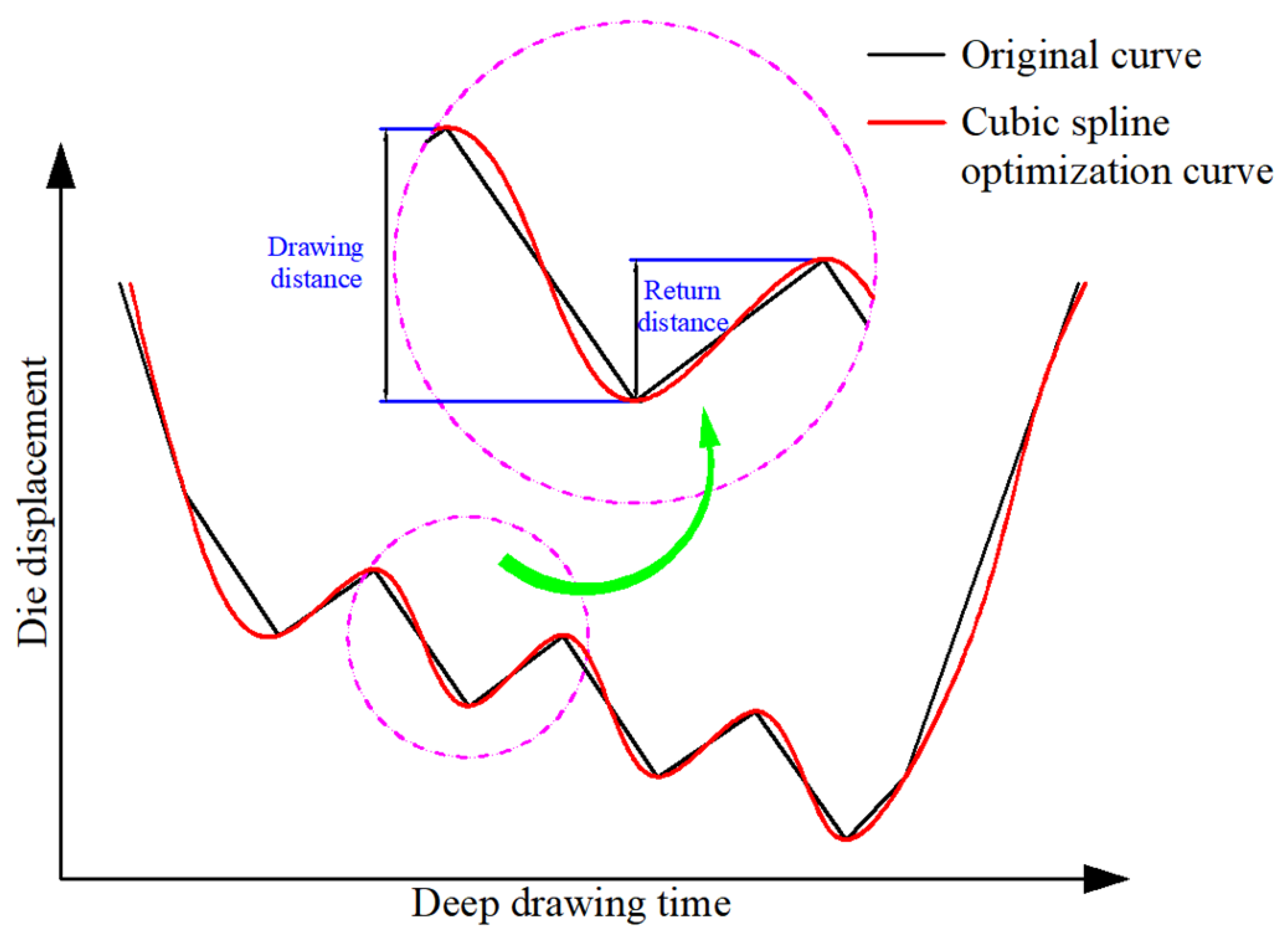
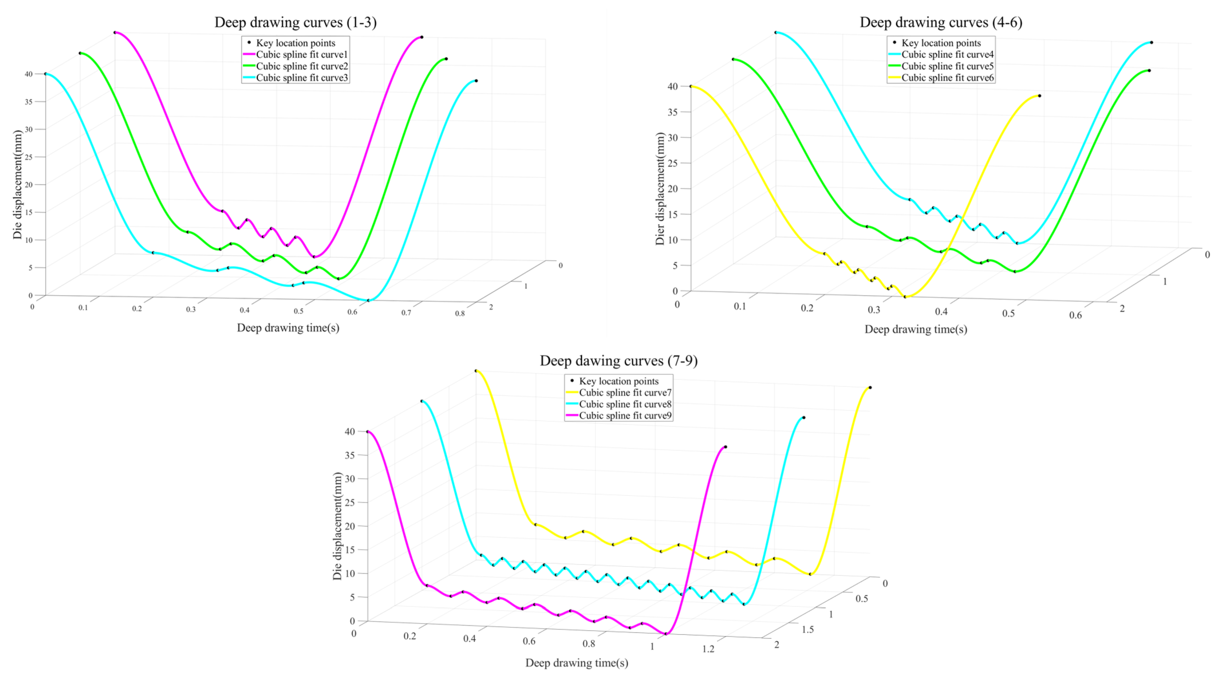
2.1. Cubic Spline Fit Optimization

If the stroke curve of the slider is obtained by linearly connecting the original key points, it will not have smoothness and high-order continuity, thus producing a significant rigid impact on the drawing process. By using a cubic spline to fit and optimize the original key points, a smooth stroke curve can be obtained, with continuous displacement speed and acceleration, allowing the slider to move more smoothly. This effectively reduces the vibration and noise generated by the press during drawing, improving the forming quality. The cubic spline curve fitting principle can be described as follows [22,23,24]:
Assuming that the cubic spline curve S ( t ) formed by the data points ( t 1 , y 1 ), ( t 2 , y 2 ), ( t 3 , y 3 ), …, ( t n , y n ) has a total of n interpolation points ( t 1 < t 2 < t 3 < … < t n 1 < t n ), then the S ( t ) can be expressed as the following set of polynomials:
S 1 ( t ) = a 1 + b 1 t t 1 + c 1 t t 1 2 + d 1 t t 1 3 , t t 1 , t 2 , S 2 ( t ) = a 2 + b 2 t t 2 + c 2 t t 2 2 + d 2 t t 2 3 , t t 2 , t 3 , S n 1 ( t ) = a n 1 + b n 1 t t n 1 + c n 1 t t n 1 2 + d n 1 t t n 1 3 , t t n 1 , t n
The following formula can be obtained by forcing continuity at the nodes:
S i t i = y i , S i t i + 1 = y i + 1 , i = 1 , 2 , n 1 . a i = y i , i = 1 , 2 , n 1 . y 2 = y 1 + b 1 t 2 t 1 + c 1 t 2 t 1 2 + d 1 t 2 t 1 3 y n = y n 1 + b n 1 t n t n 1 + c n 1 t n t n 1 2 + d n 1 t n t n 1 3
The following formula can be obtained by forcing smoothness at the nodes:
S i 1 t i = S i t i , S i 1 t i = S i t i , i = 1 , 2 , , n . 0 = S 1 t 2 S 2 t 2 = b 1 + 2 c 1 t 2 t 1 + 3 d 1 t 2 t 1 2 b 2 0 = S n 2 t n 1 S n 1 t n 1 = b n 2 + 2 c n 2 t n 1 t n 2 + 3 d n 2 t n 1 t n 2 2 b n 1 0 = S 1 t 2 S 2 t 2 = 2 c 1 + 6 d 1 t 2 t 1 2 c 2 0 = S n 2 t n 1 S n 1 t n 1 = 2 c n 2 + 6 d n 2 t n 1 t n 2 2 c n 1
Let c n = S n 1 t n / 2 and denote δ i = t i + 1 t i , Δ i = y i + 1 y i , i = 1 , 2 , , n 1 . Then, from Formula (3), we have:
d i = c i + 1 c i 3 δ i , i = 1 , 2 , , n 1 .
Furthermore, from the solution of Formula (2), we obtain:
b i = Δ i δ i c i δ i d i δ i 2 = Δ i δ i δ i 3 2 c i + c i + 1 , i = 1 , 2 , , n 1
Bringing Formulas (4) and (5) into Formula (3), we get:
δ 1 c 1 + 2 δ 1 + δ 2 c 2 + δ 2 c 3 = 3 Δ 2 δ 2 Δ 1 δ 1 δ n 2 c n 2 + 2 δ n 2 + δ n 1 c n 1 + δ n 1 c n = 3 Δ n 1 δ n 1 Δ n 2 δ n 2 .
According to the boundary conditions at the endpoints, the associated conditions can be divided into the following three categories.
(1)
The natural spline:
c 1 = 0 c n = 0
(2)
The first derivative of a given endpoint:
2 δ 1 c 1 + δ 1 c 2 = 3 Δ 1 / δ 1 S 1 t 1 δ n 1 c n 1 + 2 δ n 1 c n = 3 S n 1 t n Δ n 1 / δ n 1
(3)
The second derivative of a given endpoint:
2 δ 1 c 1 + δ 1 c 2 = 3 Δ 1 / δ 1 S 1 t 1 δ n 1 c n 1 + 2 δ n 1 c n = 3 S n 1 t n Δ n 1 / δ n 1
Here, b i , c i , and d i can be solved by combining Equation (6) with the selected boundary conditions. Thus, the cubic spline fitting curve for each sub-interval can be obtained.

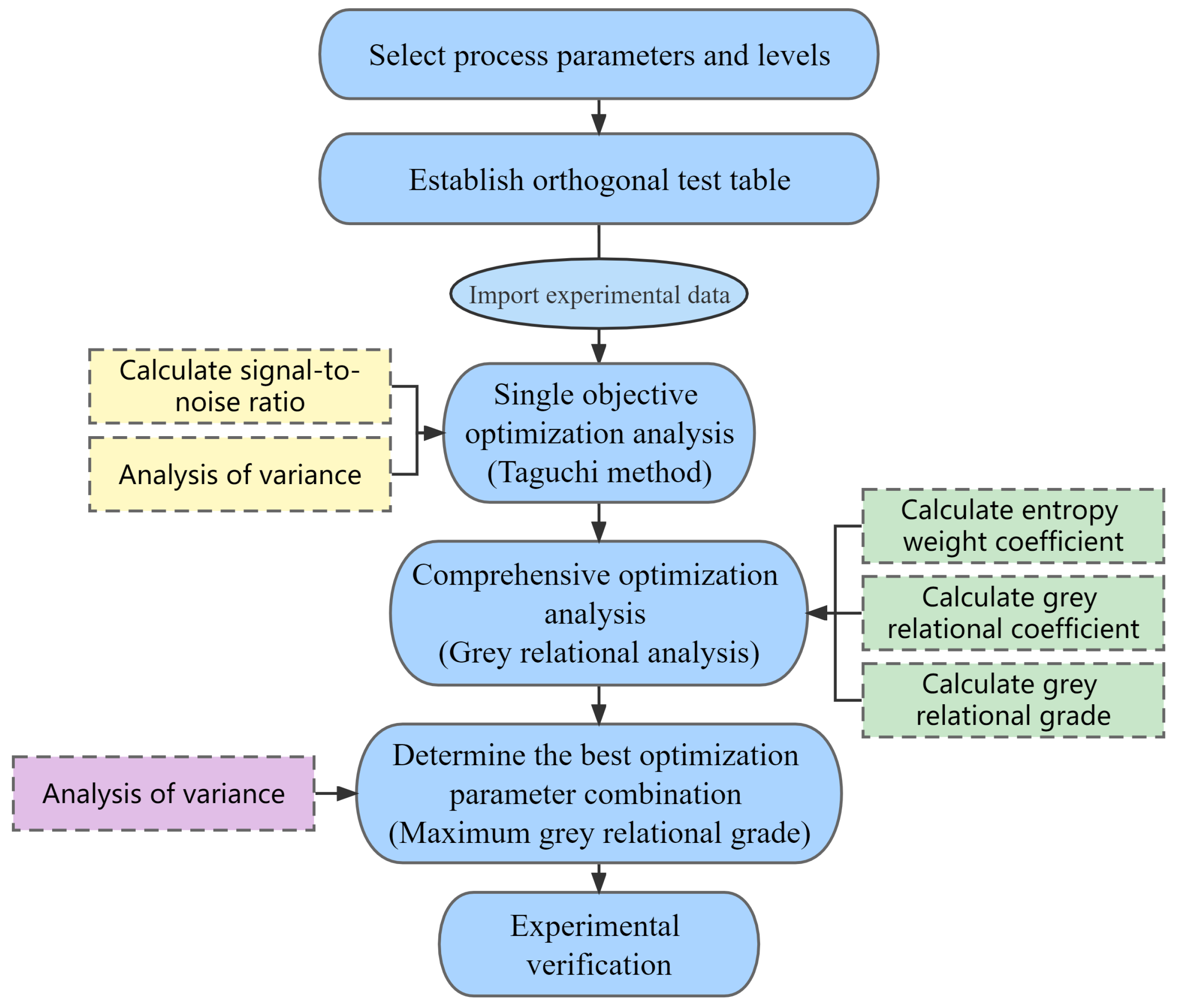
2.2. Taguchi Grey Relational Optimization Method

The Taguchi method is a quality management optimization method created by Dr. Taguchi Genichi. It has been widely used in many industries, such as the aerospace, automobile, electronics, and chemical industries. It can achieve the purpose of parameter optimization with fewer experiments, thus rapidly and effectively improving product quality, reducing production costs, and shortening the research period. The Taguchi method is generally divided into three design stages—namely, system design, parameter design, and tolerance design—where parameter design is the core and emphasis. In the parameter design, the optimal parameter combination is obtained through a Taguchi orthogonal experimental design and signal-to-noise ratio analysis, following which the parameter combination is applied to the optimized object to improve its quality level [25]. In the optimization step, the quality characteristic is the focus of the optimization research object, which can be divided into three response indicators: nominal is best, larger is better, or smaller is better. In the nominal-is-best case, there is a fixed target value, and it is hoped that the quality characteristic will come infinitely close to the target value. In the smaller−is−better case, the quality characteristics should be minimized, where the ideal value is zero. In the larger-is-better case, the quality characteristics should be maximized, with the ideal value being positive infinity. In this study, the maximum wear depth and deep drawing time should be as small as possible, meaning that we consider the smaller−is−better case [26]. In the Taguchi method, common analysis indices include the signal−to−noise ratio and sensitivity. Dr. Taguchi borrowed the definition of signal−to−noise ratio in the communications industry and applied it to the analysis in the Taguchi test. As a stability index of product quality characteristics, it is an important tool for parameter design. According to the original definition of the signal−to−noise ratio and the quality characteristics of response, the calculation formula for the signal−to−noise ratio differs, where the specific definitions are as follows [27]:
(1)
Nominal−is−best case:
η = 10 log μ 2 σ 2 , μ = 1 n i = 1 n y i , σ = 1 n 1 i = 1 n y i μ 2 ,
where η represents the signal-to-noise ratio (s/n), μ is the mean value of the response of the test group, σ is the standard deviation of the response of the test group, y i is the mass response value in the i th test, and n is the number of tests in each experiment.
(2)
Larger−is−better case:
η = 10 log 1 n i = 1 n 1 y i 2 .
(3)
Smaller−is−better case:
η = 10 log 1 n i = 1 n y i 2 .
Although the Taguchi method can be used to optimize a certain quality characteristic, it cannot deal with the problem of comprehensive optimization of multiple quality characteristics, especially when the results for each optimization parameter combination are quite different. In this case, it is necessary to use Taguchi grey relational analysis for comprehensive optimization analysis. Grey relational analysis (GRA) originated from grey system theory, created by Dr. Deng Julong. Grey relational analysis refers to the quantitative description and comparison of a system’s development and changes. It can make up for the shortcomings of statistical regression, and can judge whether their relationship is close or not by referring to the similarity in the geometric shapes of data columns, using several comparison data columns in order to effectively analyze the corresponding relationship between each series [28].
The basic process of Taguchi grey relational analysis is described in the following.
Before the data analysis, the data in each experimental data column in the system may differ in dimension, such that it is inconvenient to compare or difficult to obtain a correct conclusion during comparison. Therefore, the experimental data should be dimensionless and normalized. Treatment methods are mainly divided into the following three categories [29].
(1)
The higher the better:
x i ( k ) = y i ( k ) min y i ( k ) max y i ( k ) min y i ( k ) .
(2)
Nominal is best:
x i ( k ) = 1 y i ( k ) y e ( k ) max y i ( k ) y e ( k )
(3)
The lower the better:
x i ( k ) = max y i ( k ) y i ( k ) max y i ( k ) min i ( k )
where i = 1 , 2 , , n , k = 1 , 2 , , m , x i ( k ) is the normalized value of the k th quality characteristic in the i th sequence, y e ( k ) is the expected value of the quality characteristic, max y i ( k ) is the maximum value of y i ( k ) , min y i ( k ) is the minimum value of y i ( k ) , n is the number of experiments, and m is the number of quality characteristics.
After the original data are normalized, the grey relational coefficient of each sequence can be calculated. The calculation formula for the grey relational coefficients is as follows [30]:
ξ i ( k ) = min k min i x 0 ( k ) x i ( k ) + ρ max k max i x 0 ( k ) x i ( k ) x 0 ( k ) x i ( k ) + ρ max k max i x 0 ( k ) x i ( k ) ,
where ξ i ( k ) is the grey correlation coefficient of the i th sequence and ρ is the resolution coefficient. The smaller the value of ρ , the greater the resolution (usually, ρ = 0.5 ).
Finally, the grey relational coefficients can be used to calculate the grey relational grade, which is calculated as follows:
γ i = k = 1 m w k ξ i ( k ) i = 1 , , n ,
where w k is the entropy weight of the k th factor. As the importance of each quality characteristic may be different, in order to compare the importance of each quality characteristic, the weight obtained from entropy measurement is needed.
In information theory, entropy describes the degree of disorder of information in a system. The greater the entropy value, the greater the diversity of system responses, the higher the utility value of information and, therefore, the greater its weight. In grey relational analysis, the entropy method can be used to determine the weight coefficient of each factor. The calculation process of the entropy method is as follows.
The entropy mapping function is defined as follows [31]:
W e ( x ) = X e ( 1 x ) + ( 1 x ) e x 1 .
When x takes a value of 0.5, the function is maximized. In order to produce a mapping result in the range [ 0 , 1 ] , the entropy function is defined as:
W 1 e 0.5 1 n i = 1 n w e x i .
Then, we calculate the entropy value of each quality characteristic as:
e k = 1 e 0.5 1 × n i = 1 n w e ξ i ( k ) i = 1 n ξ i ( k ) , k = 1 , 2 , , m .
Finally, the weight coefficient of each quality characteristic is calculated as:
w k = 1 / m k = 1 m e k 1 e k k = 1 m 1 / m k = 1 m e k 1 e k , k = 1 , 2 , , m .
The above provides the necessary calculation steps and methods for Taguchi grey relational analysis. In this research, given that multiple optimization objects (wear depth and drawing time) are considered, as the Taguchi method can only optimize a single object, we need to combine the Taguchi method and grey relational analysis to solve the multi-objective optimization problem. The basic flow of this method is shown in Figure 1. First, we set the components of the pulse curve; take the drawing depth, drawing speed, return height, and return speed as the pulse curve process parameters; change the process parameters to control the shape of the curve. The orthogonal table with three levels and four factors was set using the Minitab software (Version: 17.1.0, Minitab LLC., State College, PA, USA). The results of finite element simulation analysis were imported into the software for analysis of variance, and the influence degree of each process parameter on the quality characteristics (optimized objects) and the single-objective optimal parameter combination were obtained. Then, the grey relational coefficient for each group of experiments and the entropy weight coefficient for the quality characteristics were calculated, and the grey relational degree for each group of experiments was obtained. Through analysis of variance, the optimal parameter combination for multi-objective optimization was obtained; namely, that which had the largest grey relational degree among all experimental groups. Finally, the actual effect under the optimized parameter combination was verified through a deep drawing experiment.

3. Experiment Details

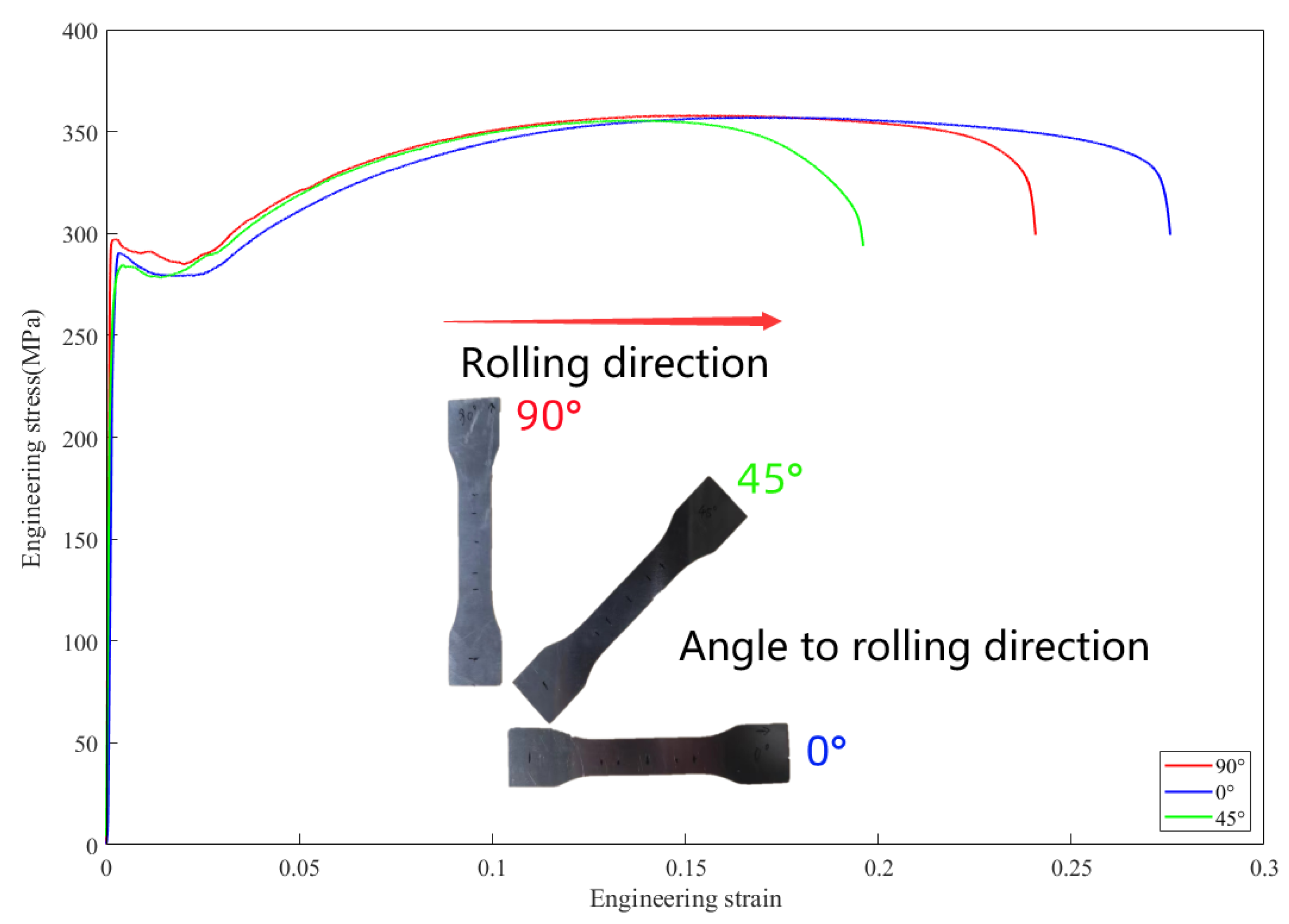
3.1. Test for Material Property

In order to accurately predict the deformation process of tantalum drawing in the finite element simulation, it was necessary to test the basic mechanical properties of the used tantalum plate. The material used in this experiment was a thin tantalum plate with a thickness of 0.2 mm. This tantalum plate was cut into dog-bone samples with three different directions (angles of 0°, 45°, and 90° in the rolling direction) by wire cutting, following which tensile tests of the samples were carried out on a universal tensile testing machine (MTS-SANSCMT6104, Xinsansi Enterprise Development Co., Ltd, Shanghai, China), until the samples broke. Three parallel tests were conducted on each sample, and the sample with the most repeatable stress–strain curve was selected for the final test data. The stress–strain data in three directions are shown in Figure 2, and the basic mechanical performance parameters are provided in Table 1.
After obtaining the basic mechanical properties parameters of the tantalum plate, we also needed to process the anisotropic parameters of tantalum, in order to convert them into input parameters conforming to the Hill-48 yield criterion. The converted parameters are shown in Table 2. The Hill-48 yield criterion is a yield criterion considering the anisotropic behavior of materials. The form of this criterion is simple and it is suitable for describing the yield behavior of orthotropic materials. Its expression is as follows [32]:
F σ y y σ z z 2 + G σ z z σ x x 2 + H σ x x σ y y 2 + 2 L σ y z 2 + 2 M σ z x 2 + 2 N σ x y 2 = σ ¯ 2 ,
F = 1 2 1 R 22 2 + 1 R 33 2 1 R 11 2 , G = 1 2 1 R 33 2 + 1 R 11 2 1 R 22 2 , H = 1 2 1 R 11 2 + 1 R 22 2 1 R 33 2 , L = 3 2 R 23 2 , M = 3 2 R 13 2 , N = 3 2 R 12 2 ,
where x, y, and z are the main axes of anisotropy; F, G, H, L, M, and N are independent anisotropy coefficients, where the coefficient values of different materials are different; and R 11 , R 22 , R 33 , R 12 , R 13 , and R 23 are six yield stress factors in plane stress state.

3.2. Material Constitutive Equation

The material constitutive equation is a mathematical relationship used to describe the mechanical properties of materials, which can reflect the yield criterion, hardening law, and stress–strain relationship of the material. Most metal materials have different mechanical behaviors at different strain rates and temperatures, and the constitutive equation can express the mechanical properties of materials in mathematical form. At present, the Johnson–Cook (JC) and Zerilli–Armstrong (ZA) constitutive models are widely used for tantalum materials. As the JC model is considered very suitable for the numerical simulation of materials, it was adopted as the constitutive equation of tantalum in this paper.
The flow stress in the JC constitutive model is defined as follows [33]:
σ e q = A + B ε p n 1 + C ln ε ˙ p ε ˙ p r 1 ( T T r T m T r ) m ,
where ε p is the equivalent plastic strain, ε ˙ p / ε ˙ p r is the dimensionless strain rate, T r is the reference temperature, T m is the melting point temperature of the material, and A, B, n, C, and m are the constants of the model.
Through processing the data obtained from relevant experiments, the constitutive model parameters of tantalum were obtained, as shown in Table 3.

3.3. Servo Deep Drawing Pulse Curve Design

Ordinary mechanical presses cannot control the drawing speed and drawing time arbitrarily and, thus, cannot provide a good deep drawing stroke curve for the formation of products. Servo presses make up for this shortage of mechanical presses, allowing for arbitrary editing of the slider speed and displacement, thus providing suitable drawing curves for different products. At present, for servo stroke curve optimization, in order to improve the forming quality and forming accuracy, a pulse stroke curve can be generally used, which can reduce the influence of work hardening and the resistance in the process of sheet metal flow deformation through the use of a proper return stroke. At the same time, due to the vacuum effect, lubricating oil can be sucked into the mold cavity in time to achieve a better lubrication effect, thus further reducing the occurrence of adhesive wear. In order to explore the influence of different pulse curves on the adhesive wear of tantalum drawing and to find the best pulse drawing stroke curve, the drawing distance (A), drawing speed (B), return distance (C), and return speed (D) were taken as the basic components of pulse drawing curve, while the drawing time and maximum wear depth were taken as the optimization parameters. The pulse drawing curve design and optimization principle are depicted in Figure 3. Based on the Taguchi method, the pulse curve parameter table with three levels and four factors (Table 4), was set and the pulse curve parameters were standardized. Table 5 shows an orthogonal test group, designed according to Table 4 and the Taguchi method. Figure 4 shows nine pulse servo pulse stroke curves obtained after parameter design and cubic spline optimization.

3.4. Wear Model and FEM Analysis

The nine servo curves obtained above were imported into the finite element software for simulation and analysis. The basic conditions and parameters are shown in Table 6, while Figure 5 shows the structural diagram of the simulated drawing die. Its basic structure consisted of seven parts: upper compression spring, counter punch, die, sheet metal, blank holder, punch, and lower compression spring. During the deep drawing process, the counter punch is used to hold the sheet metal against the upper surface of the punch, while the blank holder is used to press the sheet metal to prevent the surface of the workpiece from wrinkling. In the finite element analysis, in order to predict the wear depth, we conducted wear prediction based on the Archard wear model, which can better reflect the adhesive wear in deep drawing. Archard’s classic equation is defined as follows [34]:
w = K H · σ N · v r d t ,
where w is the wear depth, σ N is normal compressive stress, v r is the absolute value of the relative slip rate, K is the wear coefficient, and H is the hardness of the material.
After establishing the wear model and setting the relevant experimental conditions, the nine deep drawing pulse stroke curves were tested by finite element simulation. After the finite element simulation was completed, the deep drawing time, maximum wear depths of the die and product, and other data results were recorded.

4. Results and Discussion

4.1. Wear Simulation Results

Figure 6 shows the changes in the maximum wear depth of the punch, die, and product under the nine curve modes. Under the action of different deep drawing pulse stroke curves, the maximum wear depths of the punch, die, and product after drawing differed. It can be seen from the figure that the maximum wear depth of the punch surface was much smaller than that of the female die. This is because, as the active die, it has a large relative sliding distance and speed, compared with the tantalum plate; while, at the same time, it bears large contact stress. However, the bottom surface of the tantalum plate is always attached to the punch surface, due to the pressure of the counter punch, and the tantalum plate is constantly coated on the punch surface during the deep drawing process, such that the relative sliding distance is small. Of course, it can also be found, from the figure, that the maximum wear depth of the die was highly correlated with the maximum wear depth of the product; that is, as the wear depth of the product increases, the maximum wear depth of the die increases correspondingly. However, as the hardness of the die was much greater than that of the tantalum plate, the maximum wear depth of the product surface was much greater than that of the die surface. Therefore, we took the maximum wear depth of the product as an optimization objective. Figure 7 shows the wear distribution over the tantalum plate under the nine pulse drawing stroke curves (due to the rotational symmetry of the drawing parts, a quarter model of the drawing products is provided for observation). From this figure, we can see the wear distribution law and wear risk areas of the drawing products with different curve patterns. Due to the anisotropic influence of the materials, the uneven flow of materials in the drawing process led to differences in the wear distribution areas and wear degrees on the surface of the products. It can be observed from the figure that the most seriously worn areas of the nine products were located at the straight wall near the bottom of the cup in the rolling direction of the tantalum plate.

4.2. Analysis of Variance

Taking the maximum wear depth and deep drawing time of the product as quality characteristics, the quality characteristics shown in Table 7 and their corresponding signal−to−noise ratio values were obtained. The smaller the two quality characteristics, the better the signal-to-noise ratio conversion. Table 8 shows the analysis of variance for the deep drawing time. Variance analysis was used to analyze the influence degree and contribution rate of different process parameters on quality characteristics, in order to determine the process parameters that had the greatest influence on the quality characteristics. The variance data in Table 8 show that the drawing speed (B) had the most significant influence on drawing time, with contribution rate reaching 47.5934%. Figure 8 shows the response diagram of quality characteristics to drawing time. It can be seen from this diagram that the best parameter combination was A 1 B 1 C 3 D 1 ; that is, a drawing depth of 3 mm, drawing speed of 100 mm/s, return height of 0.5 mm, and return speed of 100 mm/s. Table 9 provides the variance data for the maximum wear depth. The data in this table indicate that the return height (C) had the most significant influence on the maximum wear depth of the product, with contribution rate reaching 39.7731%, followed by the drawing depth, with contribution rate reaching 35.4619%. Figure 9 shows the quality characteristic response diagram for the maximum wear depth. It can be seen from this diagram that the best parameter combination was A 1 B 3 C 3 D 2 with the maximum wear depth as the quality objective; that is, a drawing depth of 3 mm, drawing speed of 25 mm/s, return height of 0.5 mm, and return speed of 50 mm/s.

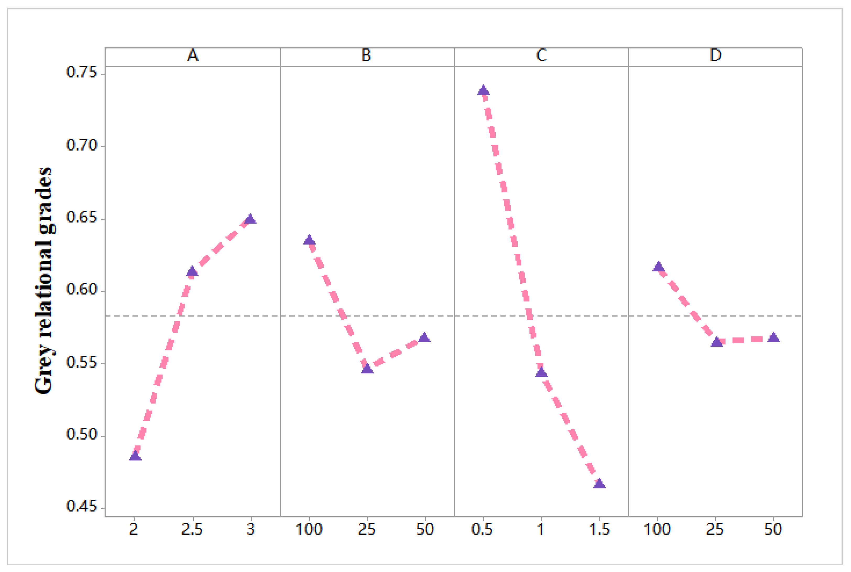
4.3. Comprehensive Optimization Analysis

From the above optimization analysis results, it can be observed that the best parameter combination for drawing time optimization was A 1 B 1 C 3 D 1 , while the best parameter combination for wear depth optimization was A 1 B 3 C 3 D 2 . Obviously, there was an inconsistency between the two optimization results, as the traditional Taguchi method cannot be used for the comprehensive optimization of multiple quality characteristics; however, Taguchi grey relational analysis can better address this task. Table 10 shows the grey relational coefficient and grey relational grade for each experimental group. In the table, it can be seen that the entropy weight of drawing time (0.528) was greater than that of maximum wear depth (0.472). Figure 10 shows the quality characteristic response diagram of the grey relational grade. It can be seen from the figure that the parameter combination with the highest grey relational grade was A 1 B 1 C 3 D 1 , and Table 11 shows the variance results for the relational grade. The data in Table 11 indicate that the return height (C) had the greatest influence on the maximum wear depth of the product, with a contribution rate of 63.5484%, followed by the drawing depth (A), with a contribution rate of 23.9785%, while the drawing speed (B) and return speed (D) had very small contribution rates. However, in the single-objective analysis, drawing speed had the greatest influence on the maximum wear depth. In order to reduce the influence of drawing speed on the wear depth, A 1 B 2 C 3 D 1 was finally selected as the optimal parameter combination after optimization; that is, a drawing depth of 3 mm, drawing speed of 50 mm/s, return height of 0.5 mm, and return speed of 100 mm/s. Figure 11 shows the change in grey relational grade between the nine experimental parameter combinations (1–9) before optimization and the optimized parameter combination (10). It can be seen from the figure that the optimized grey relational grade value was 0.89, which was the highest among all parameter combinations, thus achieving the purpose of comprehensive optimization.

4.4. Experimental Verification

In order to understand the experimental deep drawing effect of the optimized drawing stroke curve, we carried out experimental verification of the designed stroke curve on a servo press, where Figure 12 shows the die and servo press used for the deep drawing experiment. We compared the deep drawing time and the maximum wear depth of the product between the traditional deep drawing mode (sinusoidal stroke curve mode on common mechanical press) and the optimized deep drawing mode (pulse drawing curve mode based on the parameter combination A 1 B 2 C 3 D 1 ). Figure 13 shows the comparison of simulated and experimental deep drawing wear morphologies between traditional drawing and optimized drawing curves. It can be seen from the figure that the simulated and actual drawing effects were basically consistent, where the red circle in the figure marks the position of the maximum wear depth on the product. Figure 14 shows the macroscopic and microscopic wear morphology of products under traditional deep drawing and optimized deep drawing. Considering the macroscopic morphology of the two products (Figure 14a,b), it can be observed that the surface of the products formed using traditional deep drawing was rough, while that of the products formed under optimized deep drawing was flat and smooth. Figure 14c,d show the micro-wear morphology of the area where the red circle is located (i.e., the area with the maximum wear depth). From the micro-morphology results, the maximum wear depth of the product formed by optimized deep drawing was 11.818 μ m, while that of the surface formed by traditional deep drawing was 27.278 μ m. Therefore, compared with traditional deep drawing, the maximum wear depth with optimized deep drawing was reduced by nearly 57%. In addition, the drawing time with optimized deep drawing was 0.59 s, while that with traditional deep drawing was 0.72 s, allowing the deep drawing time to be shortened by nearly 18%. Thus, the optimized deep drawing method improved the surface quality and deep drawing efficiency of products. Table 12 provides the predicted and experimental data results for the quality characteristics under the traditional and optimized deep drawing methods in detail. From this table, it can be seen that the wear prediction error for traditional and optimized deep drawing was 8.22% and, so, the actual drawing wear could be predicted accurately, to a certain extent, through finite element simulation.

5. Conclusions

In this study, Taguchi grey relational analysis was used to optimize the adhesion and wear of tantalum deep drawing, and the influences of various pulse curve process parameters (i.e., drawing depth, drawing speed, return height, and return speed) on the quality characteristics (i.e., drawing forming time and the maximum wear depth) of the sheet metal were studied. In this way, we obtained the best combination parameters, which were applied to tantalum drawing using a servo press. Compared with traditional deep drawing, the optimized parameter combination improved the drawing efficiency and product surface quality. The specific research results can be summarized as follows:
(1)
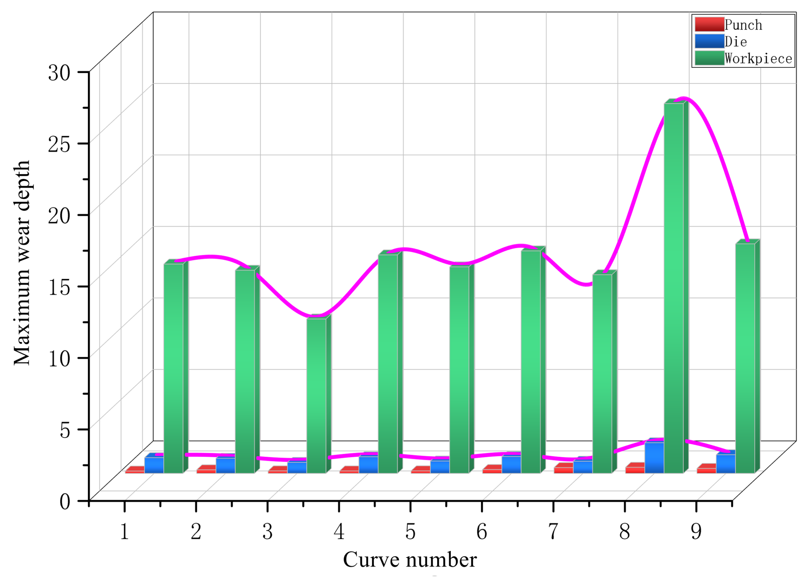
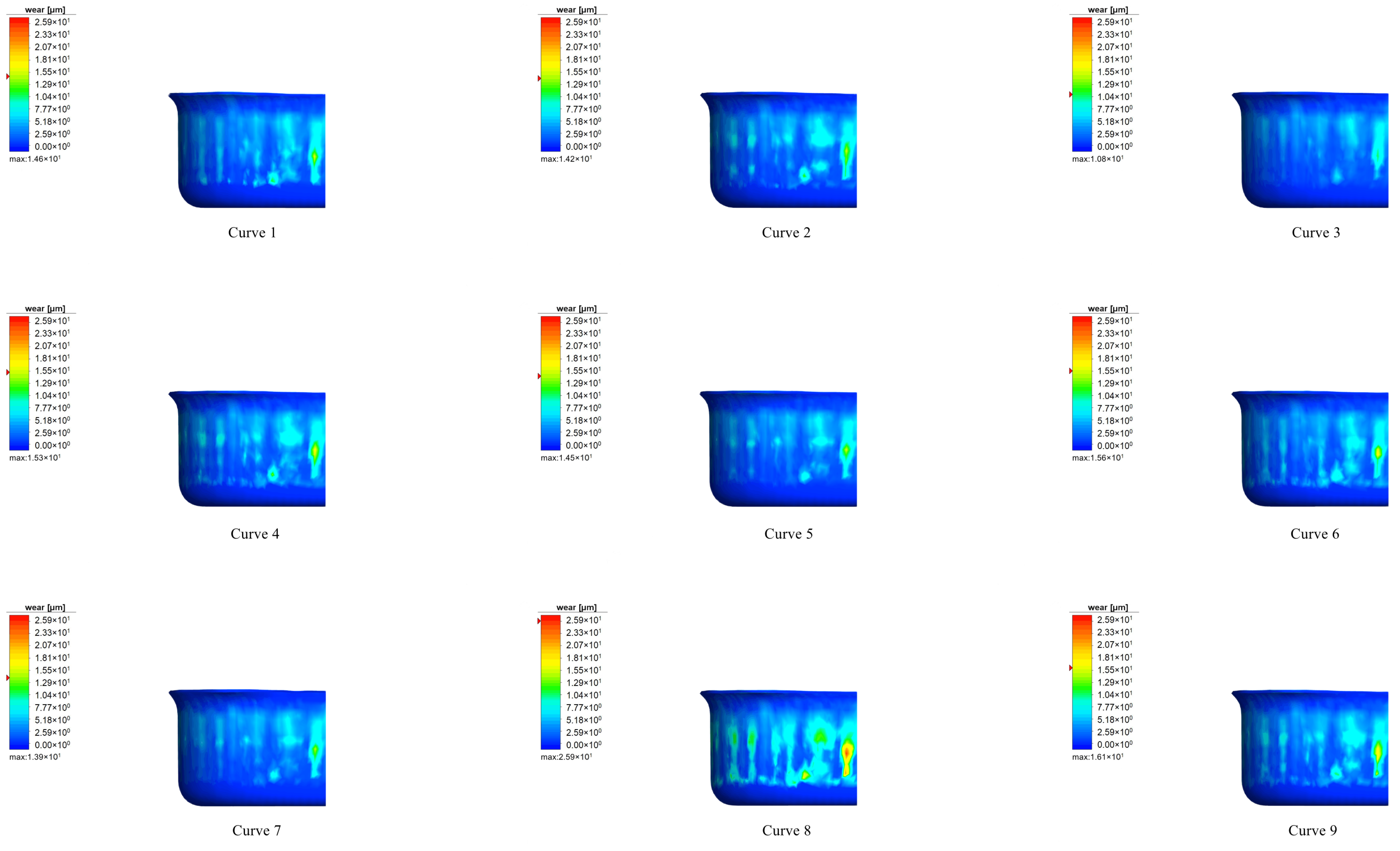
In the finite element simulation experiment of tantalum deep drawing, the wear degrees of the drawing die and product under the nine considered curve modes differed. Compared with the product surface wear, the maximum wear depth of the die surface was much smaller, while the maximum wear depth of the punch surface can be neglected. Considering the wear morphology of the product surface, the most serious wear area occurred at the straight wall near the bottom of the cup in the rolling direction of the tantalum plate.
(2)
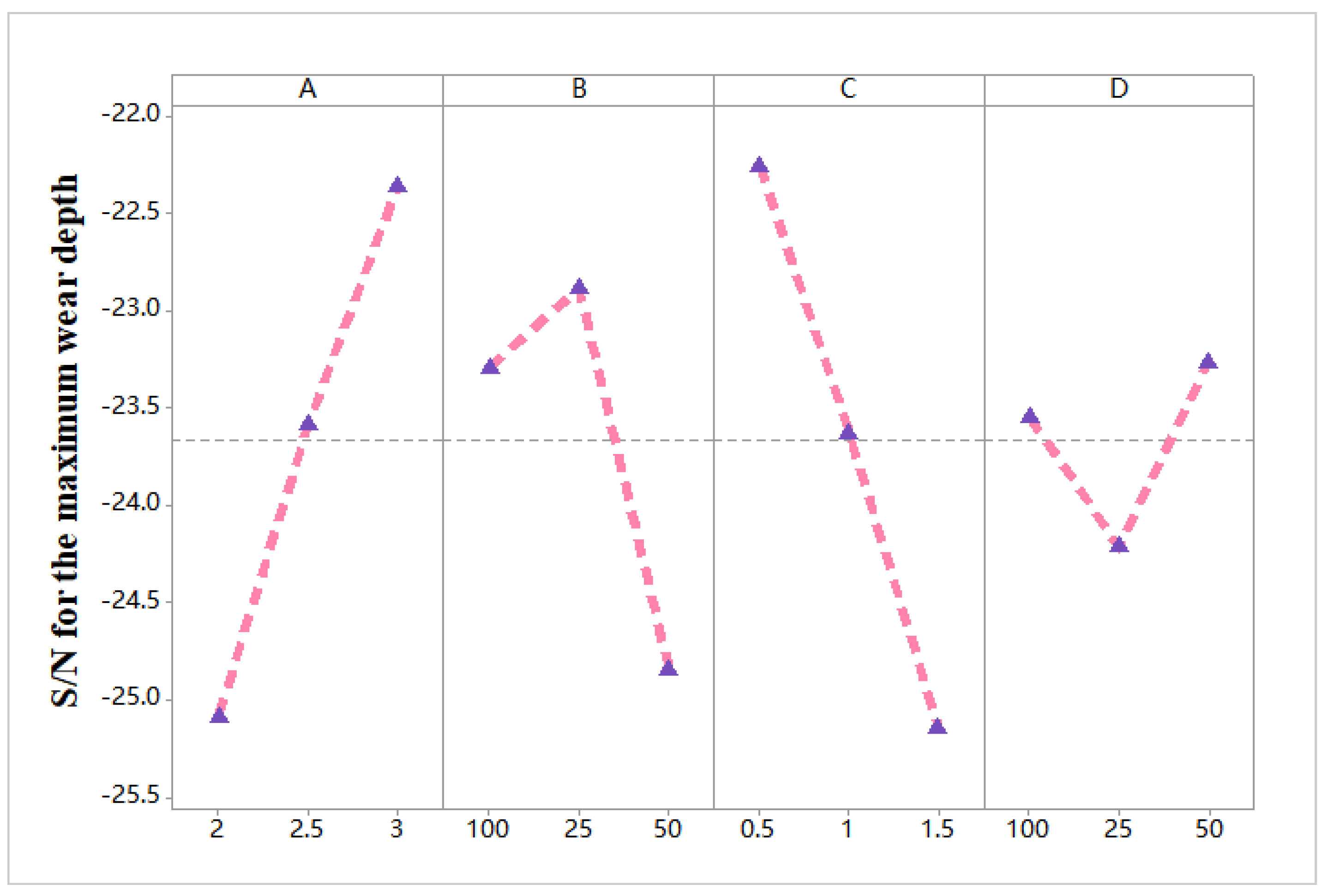
Based on the Taguchi method, with deep drawing time as the optimization objective, the best parameter combination of pulse drawing stroke curve was A 1 B 1 C 3 D 1 , leading to the shortest deep drawing time in all experimental groups; meanwhile, with wear depth as the optimization objective, the best parameter combination of pulse drawing stroke curve was A 1 B 3 C 3 D 2 . The overall best parameter combination, obtained by Taguchi grey relational analysis, was A 1 B 2 C 3 D 1 , with the grey relational grade reaching 0.89, higher than those of the other nine experiments.
(3)
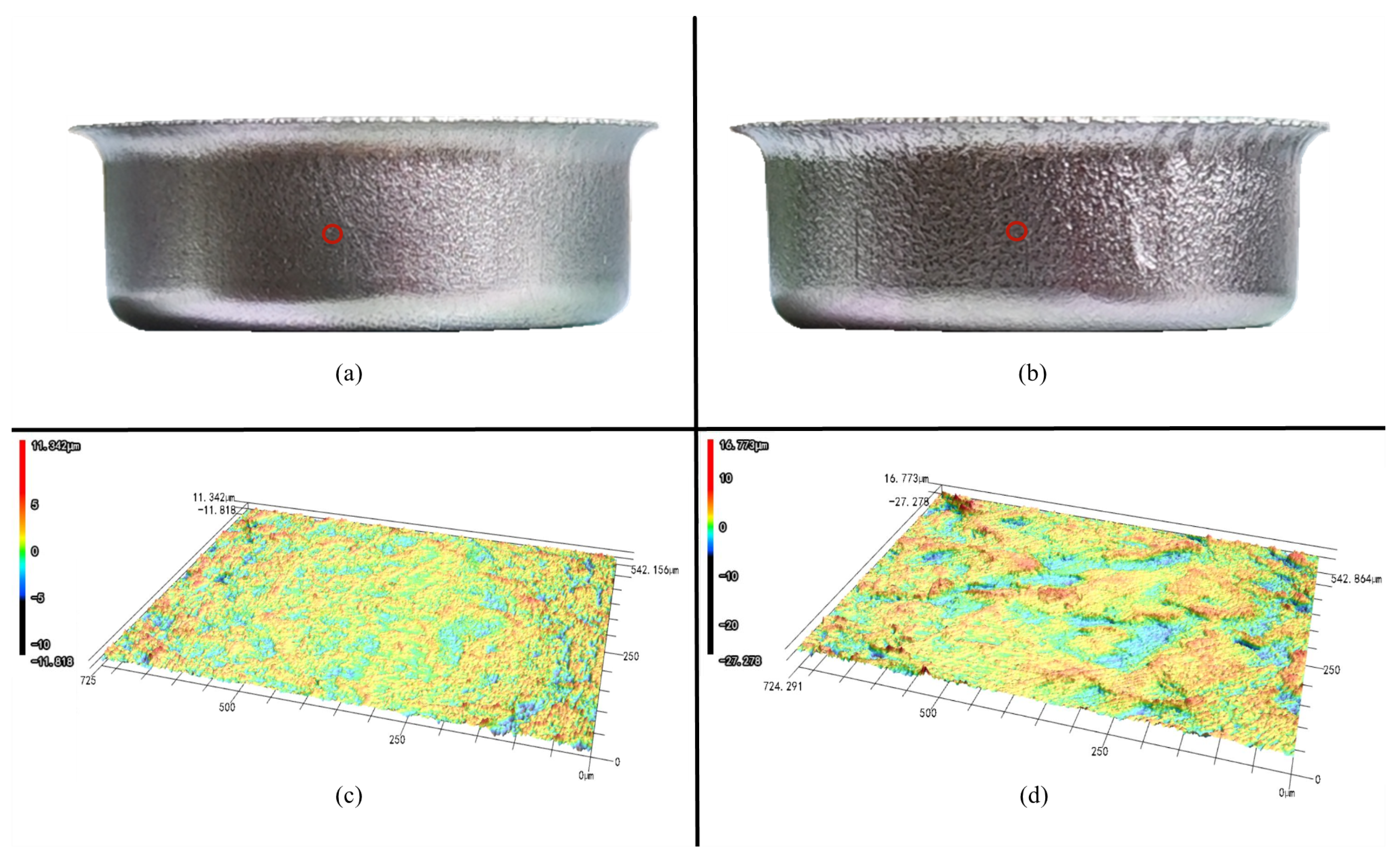
In the deep drawing verification experiment, the surface quality and the deep drawing time of products formed using the traditional drawing mode and the optimized drawing mode (A 1 B 2 C 3 D 1 ) were compared. Considering the macroscopic appearance of the deep drawing products, the surface of the traditional deep drawing product was rough, while that of the optimized deep drawing product was flat and smooth and, thus, the quality of the optimized deep drawing product was obviously better than that of the traditional deep drawing product. Considering the micro-morphology of the severely worn area, the maximum wear depth on the surface of the product formed by optimized deep drawing was 11.818 μ m, while that formed by traditional deep drawing was 27.278 μ m. Furthermore, the deep drawing time under the optimized drawing mode was 0.59 s, while that with traditional deep drawing was 0.72 s. In summary, compared with traditional deep drawing, the maximum wear depth of the product under the optimized deep drawing mode was reduced by 56.67% and the deep drawing time was shortened by 18.06%. The surface quality and deep drawing efficiency of the product were improved through the use of the optimized deep drawing mode.

Author Contributions

Conceptualization, X.W. and T.X.; methodology, X.W. and T.X.; software, X.W.; validation, X.W., T.X., F.G. and J.R.; formal analysis, X.W.; investigation, T.X. and X.W.; resources, T.X.; data curation, X.W. and T.X.; writing—original draft preparation, X.W.; writing—review and editing, X.W. and T.X.; visualization, X.W.; supervision, T.X., J.R. and F.G.; project administration, T.X., F.G. and J.R.; funding acquisition, T.X. All authors have read and agreed to the published version of the manuscript.

Funding

The work described in this paper was supported by grants from (1) National Natural Science Foundation of China (Grant No. 52005341); (2) Research Start-up Project for Newly Introduced Teachers in Shenzhen University (Project No. 2019042).

Institutional Review Board Statement

Not applicable.

Informed Consent Statement

Not applicable.

Data Availability Statement

Not applicable.

Conflicts of Interest

The authors declare no conflict of interest.

References

  1. Atul S, T.; Babu, M.L. A review on effect of thinning, wrinkling and spring-back on deep drawing process. Proc. Inst. Mech. Eng. Part B J. Eng. Manuf. 2019, 233, 1011–1036. [Google Scholar] [CrossRef]
  2. Choubey, A.K.; Agnihotri, G.; Sasikumar, C. Numerical validation of experimental result in deep-drawing. Mater. Today Proc. 2015, 2, 1951–1958. [Google Scholar] [CrossRef]
  3. Zein, H.; El Sherbiny, M.; Abd-Rabou, M. Thinning and spring back prediction of sheet metal in the deep drawing process. Mater. Des. 2014, 53, 797–808. [Google Scholar] [CrossRef]
  4. Xu, F.S.; Deng, Y.L.; Zhang, J.; Guo, X.B. Influence of Fillet-Radius and Lubrication on Stamping Quality of Multi-Recessed Aluminum Panels. In Proceedings of the Mechanics and Materials Science: Proceedings of the 2016 International Conference on Mechanics and Materials Science (MMS2016), Guangzhou, China, 15–16 October 2016; pp. 201–213. [Google Scholar]
  5. Jivan, R.; Eskandarzade, M.; Bewsher, S.; Leighton, M.; Mohammadpour, M.; Saremi-Yarahmadi, S. Application of solid lubricant for enhanced frictional efficiency of deep drawing process. Proc. Inst. Mech. Eng. Part C J. Mech. Eng. Sci. 2022, 236, 624–634. [Google Scholar] [CrossRef]
  6. Berahmani, S.; Bilgili, C.; Erol, G.; Hol, J.; Carleer, B. The effect of friction and lubrication modelling in stamping simulations of the Ford Transit hood inner panel: A numerical and experimental study. IOP Conf. Ser. Mater. Sci. Eng. 2020, 967, 012010. [Google Scholar] [CrossRef]
  7. Hashemi, S.J.; Roohi, A.H. Minimizing spring-back and thinning in deep drawing process of St14 steel sheets. Int. J. Interact. Des. Manuf. (IJIDeM) 2022, 16, 381–388. [Google Scholar] [CrossRef]
  8. Cai, K.; Wang, D. Optimizing the design of automotive S-rail using grey relational analysis coupled with grey entropy measurement to improve crashworthiness. Struct. Multidiscip. Optim. 2017, 56, 1539–1553. [Google Scholar] [CrossRef]
  9. Flegler, F.; Groche, P.; Abraham, T.; Bräuer, G. Dry Deep Drawing of Aluminum and the Influence of Sheet Metal Roughness. JOM 2020, 72, 2511–2516. [Google Scholar] [CrossRef]
  10. Buckman, R. New applications for tantalum and tantalum alloys. JOM 2000, 52, 40–41. [Google Scholar] [CrossRef]
  11. Agrawal, M.; Singh, R.; Ranitović, M.; Kamberovic, Z.; Ekberg, C.; Singh, K.K. Global market trends of tantalum and recycling methods from Waste Tantalum Capacitors: A review. Sustain. Mater. Technol. 2021, 29, e00323. [Google Scholar] [CrossRef]
  12. Teverovsky, A. Breakdown and self-healing in tantalum capacitors. IEEE Trans. Dielectr. Electr. Insul. 2021, 28, 663–671. [Google Scholar] [CrossRef]
  13. Freiße, H.; Ditsche, A.; Seefeld, T. Reducing adhesive wear in dry deep drawing of high-alloy steels by using MMC tool. Manuf. Rev. 2019, 6, 12. [Google Scholar] [CrossRef]
  14. Trzepieciński, T. Polynomial Multiple Regression Analysis of the Lubrication Effectiveness of Deep Drawing Quality Steel Sheets by Eco-Friendly Vegetable Oils. Materials 2022, 15, 1151. [Google Scholar] [CrossRef]
  15. Marchin, N.; Ashrafizadeh, F. Effect of carbon addition on tribological performance of TiSiN coatings produced by cathodic arc physical vapour deposition. Surf. Coatings Technol. 2021, 407, 126781. [Google Scholar] [CrossRef]
  16. Halicioglu, R.; Dulger, L.C.; Bozdana, A.T. Mechanisms, classifications, and applications of servo presses: A review with comparisons. Proc. Inst. Mech. Eng. Part B J. Eng. Manuf. 2016, 230, 1177–1194. [Google Scholar] [CrossRef]
  17. Li, T.C.; Kuo, C.C.; Yang, C.Y.; Liu, K.W.; Li, P.H.; Lin, B.T. Influence of motion curve errors of direct-drive servo press on stamping properties. Int. J. Adv. Manuf. Technol. 2022, 120, 4461–4476. [Google Scholar] [CrossRef]
  18. Chen, D.C.; Yeh, Y.K. Using finite element analysis to discuss the study of drawing of servo stamping curve. Adv. Mech. Eng. 2021, 13, 16878140211061015. [Google Scholar] [CrossRef]
  19. Matsumoto, R.; Jeon, J.Y.; Utsunomiya, H. Shape accuracy in the forming of deep holes with retreat and advance pulse ram motion on a servo press. J. Mater. Process. Technol. 2013, 213, 770–778. [Google Scholar] [CrossRef]
  20. Kuo, C.C.; Huang, H.L.; Li, T.C.; Fang, K.L.; Lin, B.T. Optimization of the pulsating curve for servo stamping of rectangular cup. J. Manuf. Process. 2020, 56, 990–1000. [Google Scholar] [CrossRef]
  21. Halicioglu, R.; Dulger, L.C.; Bozdana, A.T. Improvement of metal forming quality by motion design. Robot. Comput. -Integr. Manuf. 2018, 51, 112–120. [Google Scholar] [CrossRef]
  22. Habib, Z.; Sarfraz, M.; Sakai, M. Rational cubic spline interpolation with shape control. Comput. Graph. 2005, 29, 594–605. [Google Scholar] [CrossRef]
  23. Kirsiaed, E.; Oja, P.; Shah, G.W. Cubic spline histopolation. Math. Model. Anal. 2017, 22, 514–527. [Google Scholar] [CrossRef]
  24. Zhanlav, T.; Mijiddorj, R. A comparative analysis of local cubic splines. Comput. Appl. Math. 2018, 37, 5576–5586. [Google Scholar] [CrossRef]
  25. Padmanabhan, R.; Oliveira, M.; Alves, J.; Menezes, L. Influence of process parameters on the deep drawing of stainless steel. Finite Elem. Anal. Des. 2007, 43, 1062–1067. [Google Scholar] [CrossRef]
  26. Bouchaâla, K.; Ghanameh, M.F.; Faqir, M.; Mada, M.; Essadiqi, E. Prediction of the impact of friction’s coefficient in cylindrical deep drawing for AA2090 Al-Li alloy using FEM and Taguchi approach. IOP Conf. Ser. Mater. Sci. Eng. 2019, 664, 012004. [Google Scholar] [CrossRef]
  27. Ren, J.; Zhou, J.; Zeng, J. Analysis and optimization of cutter geometric parameters for surface integrity in milling titanium alloy using a modified grey–Taguchi method. Proc. Inst. Mech. Eng. Part B J. Eng. Manuf. 2016, 230, 2114–2128. [Google Scholar] [CrossRef]
  28. Pillai, J.U.; Sanghrajka, I.; Shunmugavel, M.; Muthuramalingam, T.; Goldberg, M.; Littlefair, G. Optimisation of multiple response characteristics on end milling of aluminium alloy using Taguchi-Grey relational approach. Measurement 2018, 124, 291–298. [Google Scholar] [CrossRef]
  29. Mahdaviani, S.H.; Parvari, M.; Soudbar, D. Simultaneous multi-objective optimization of a new promoted ethylene dimerization catalyst using grey relational analysis and entropy measurement. Korean J. Chem. Eng. 2016, 33, 423–437. [Google Scholar] [CrossRef]
  30. Chiang, Y.M.; Hsieh, H.H. The use of the Taguchi method with grey relational analysis to optimize the thin-film sputtering process with multiple quality characteristic in color filter manufacturing. Comput. Ind. Eng. 2009, 56, 648–661. [Google Scholar] [CrossRef]
  31. Wen, K.L.; Chang, T.C.; You, M.L. The grey entropy and its application in weighting analysis. In Proceedings of the 1998 IEEE International Conference on Systems, Man, and Cybernetics (Cat. No. 98CH36218), San Diego, CA, USA, 14 October 1998; Volume 2, pp. 1842–1844. [Google Scholar]
  32. Karajibani, E.; Fazli, A.; Hashemi, R. Numerical and experimental study of formability in deep drawing of two-layer metallic sheets. Int. J. Adv. Manuf. Technol. 2015, 80, 113–121. [Google Scholar] [CrossRef]
  33. Chen, S.R.; Gray, G.T. Constitutive behavior of tantalum and tantalum-tungsten alloys. Metall. Mater. Trans. A 1996, 27, 2994–3006. [Google Scholar] [CrossRef]
  34. Aghababaei, R.; Zhao, K. Micromechanics of material detachment during adhesive wear: A numerical assessment of Archard’s wear model. Wear 2021, 476, 203739. [Google Scholar] [CrossRef]
Figure 1. Basic flow diagram of comprehensive optimization analysis.
Metals 12 01340 g001
Figure 2. Engineering stress–strain curves of tantalum material in different directions.
Metals 12 01340 g002
Figure 3. Design and optimization of servo deep drawing stroke pulse curve.
Metals 12 01340 g003
Figure 4. Nine servo−based deep drawing pulse stroke curves.
Metals 12 01340 g004
Figure 5. Basic structure of finite element simulation model.
Metals 12 01340 g005
Figure 6. Change in maximum wear depth of punch, die, and product under different curve modes.
Metals 12 01340 g006
Figure 7. Wear distribution diagram of deep drawing products under different curve modes.
Metals 12 01340 g007
Figure 8. Signal−to−noise ratio response diagram for deep drawing time.
Metals 12 01340 g008
Figure 9. Signal−to−noise ratio response diagram for maximum wear depth.
Metals 12 01340 g009
Figure 10. Signal−to−noise ratio response diagram of grey relational grade.
Metals 12 01340 g010
Figure 11. Signal−to−noise ratio response diagram for maximum wear depth.
Metals 12 01340 g011
Figure 12. Servo press and deep drawing die.
Metals 12 01340 g012
Figure 13. Comparison of product surface morphology between drawing simulation and experiment: (a) optimized deep drawing mode; (b) traditional deep drawing mode.
Metals 12 01340 g013
Figure 14. Comparison of macroscopic and microscopic wear morphology of deep drawing product surface: (a) macro-morphology of product surface in optimized deep drawing mode; (b) macro-morphology of product surface in traditional deep drawing mode; (c) micro-morphology of products in optimized deep drawing mode; (d) micro-morphology of product surface in traditional deep drawing mode.
Metals 12 01340 g014
Table 1. Basic mechanical properties of tantalum.
Yield strength (MPa)276 ± 5
Tensile strength (MPa)350 ± 7
Young’s modulus (GPa)186 ± 4
Poisson’s ratio0.35 ± 0.01
Table 2. Anisotropy parameters of tantalum.
Plastic strain ratio0.87 (0°)Yield stress factorR 11 1.0272
0.8 (45°)R 22 0.9886
0.6614 (90°)R 33 0.9231
Yield strength (MPa)273 (0°)R 12 0.9916
272 (45°)R 13 1.0
283 (90°)R 23 1.0
Table 3. Parameters of JC constitutive model for tantalum plate.
A (MPa)B (MPa)CmnT r (°C)T m (°C) ε ˙ p r
241.87447.50.0570.880.52529710.001
Table 4. Control factors and levels of deep drawing pulse curves.
Controlling FactorsLevels
123
Deep drawing depth (A; mm)32.52
Deep drawing speed (B; mm/s)1005025
Return height (C; mm)1.510.5
Return speed (D; mm/s)1005025
Table 5. Orthogonal test table for nine sets of pulse drawing curve parameters.
Curve No.A (mm)B (mm/s)C (mm)D (mm/s)
131001.5100
2350150
33250.525
42.5100125
52.5500.5100
62.5251.550
72000.550
82501.525
92251100
Table 6. Basic condition parameters for FEM simulation.
Sheet metal diameter (mm)32.4
Sheet thickness (mm)0.2
Model sizePunch diameter (mm)20
Die diameter (mm)20.42
Die clearance (mm)0.22
Thermal conductivity of tantalum (W/(m·K))54.4
Thermal propertiesSpecific heat capacity of tantalum (J/(g·K))0.153
Plastic deformation dissipation coefficient0.9
Upper spring stiffness (N/m)25,000
Other conditionsLower spring stiffness (N/m)100,000
Simulated experimental temperature (°C)25
Friction coefficient0.2
Wear conditionsCoefficient of wear0.001
Die hardness (HRC)50
Table 7. Quality characteristics and signal−to−noise ratio with different pulse curves.
Curve No.Control FactorsResponse of Quality Characteristics
A (mm)B (mm/s)C (mm)D (mm/s)Deep Drawing
Time (s)
S/N (dB)Maximum Wear Depth
(μm)
S/N (dB)
131001.51000.574.882514.646−23.3144
23501500.683.349814.214−23.0543
33250.5250.801.938210.807−20.6741
42.51001250.565.036215.287−23.6864
52.5500.51000.427.535014.450−23.1974
62.5251.5501.32−2.411515.568−23.8447
72000.5500.525.679913.901−22.8609
82501.5251.28−2.144225.869−28.2560
922511001.20−1.583616.059−24.1144
Table 8. Variance results for deep drawing time.
FactorsDegrees of Freedom
(DF)
Adjusted Sum of Squares
(Adj SS)
Adjusted Mean Squares
(Adj MS)
Contribution
(%)
A214.98987.494913.5077
B252.815426.407747.5934
C236.832018.416033.1904
D26.33473.16745.7085
Total8110.971955.4860100
Table 9. Variance results for maximum wear depth.
FactorsDegrees of Freedom
(DF)
Adjusted Sum of Squares
(Adj SS)
Adjusted Mean Squares
(Adj MS)
Contribution
(%)
A211.21125.605635.4619
B26.39963.199820.2424
C212.57426.287139.7731
D21.42980.71494.5226
Total831.614715.8074100
Table 10. Simulation results of quality characteristics in deep drawing with different curves.
Curve No.Grey Relational CoefficientsGrey Relational GradeRank
Deep Drawing Time (s)Maximum Wear Depth (mm)
Weight Coefficient: 0.47Weight Coefficient: 0.53
10.65220.58950.62214
20.543020.61430.57726
30.470510.72472
40.66560.55720.61355
510.60040.80811
60.33330.54460.43478
70.72830.63420.68313
80.33940.33330.33659
90.35290.52420.43517
Table 11. Results of variance for grey relational grade.
FactorsDegrees of Freedom
(DF)
Adjusted Sum of Squares
(Adj SS)
Adjusted Mean Squares
(Adj MS)
Contribution
(%)
A214.98987.494913.5077
B252.815426.407747.5934
C236.832018.416033.1904
D26.33473.16745.7085
Total8110.971955.4860100
Table 12. Predicted and experimental result analysis for quality characteristics under traditional and optimized deep drawing modes.
Deep Drawing ModeQuality Characteristic
Deep Drawing Time (s)Maximum Wear Depth (μm)
FEMTraditional0.7224.725
Optimization0.5910.982
EXPTraditional0.7227.278
Optimization0.5911.818
Reduction (%)18.0656.67
Prediction error (%)8.22
Publisher’s Note: MDPI stays neutral with regard to jurisdictional claims in published maps and institutional affiliations.

