Strip Steel Surface Defects Classification Based on Generative Adversarial Network and Attention Mechanism

Abstract

In a complex industrial environment, it is difficult to obtain hot rolled strip steel surface defect images. Moreover, there is a lack of effective identification methods. In response to this, this paper implements accurate classification of strip steel surface defects based on generative adversarial network and attention mechanism. Firstly, a novel WGAN model is proposed to generate new surface defect images from random noises. By expanding the number of samples from 1360 to 3773, the generated images can be further used for training classification algorithm. Secondly, a Multi-SE-ResNet34 model integrating attention mechanism is proposed to identify defects. The accuracy rate on the test set is 99.20%, which is 6.71%, 4.56%, 1.88%, 0.54% and 1.34% higher than AlexNet, VGG16, ShuffleNet v2 1×, ResNet34, and ResNet50, respectively. Finally, a visual comparison of the features extracted by different models using Grad-CAM reveals that the proposed model is more calibrated for feature extraction. Therefore, it can be concluded that the proposed methods provide a significant reference for data augmentation and classification of strip steel surface defects.

1. Introduction

As one of the main products of the steel industry, hot rolled strip steel is widely used in automobile manufacturing, aerospace and light industry [1]. Surface quality is one of the key indicators of strip steel’s market competitiveness. Due to the influence of raw materials, rolling process and external environment, the strip steel surface will inevitably appear oxide scale, inclusion, scratch and other defects in the production process, which not only seriously affects the appearance, but also reduces the fatigue resistance. At the same time, these shortcomings cannot be completely overcome by improving the process [2,3]. Therefore, the classification of surface defects can provide an important reference for the production process. Through the corresponding tuning, the purpose of further improving the yield rate and reducing production costs is achieved.

The traditional surface defect detection mainly relies on manual visual inspection [4]. Although the implementation of this method is relatively simple, it is difficult to detect small defects with the continuous acceleration of the production line. In addition, long-term manual work will lead to visual fatigue and affect physical and mental health. Many researchers have used machine learning algorithms to overcome the drawbacks of manual visual inspection. Kim et al. [5] developed a K-Nearest Neighbor (KNN) classifier for eight defects with a classification performance of about 85%. Karthikeyan et al. [6] proposed a texture-based approach, where discrete wavelet transform based local configuration pattern features were given as input to a KNN classifier with an overall accuracy of 96.7%. Martins et al. [7] adopted principal component analysis to extract features from the defect images and used self-organizing maps to classify six types of defects obtained in the ArcelorMittal mill with an overall accuracy of 87%. Bulnes et al. [8] proposed a non-invasive system based on computer vision, which uses a neural network for classification and a genetic algorithm to determine the optimal values of the parameters. This method improves flexibility and the whole process can be executed quickly. Hu et al. [9] extracted geometric features, shape features, texture features and grey-scale features from defect images and their corresponding binary images. A classification model was developed by combining a hybrid chromosome genetic algorithm and a support vector machine (SVM) classifier, achieving a higher average prediction accuracy than that of the traditional SVM-based model. Jiang et al. [10] proposed an adaptive classifier with Bayesian kernel. Firstly, abundant features were introduced to cover detailed information of defects, and then a series of SVMs were constructed by using the random subspace of features. Finally, an improved Bayesian classifier was trained by fusing the results of basic SVMs, which has a strong adaptive capability. Zaghdoudi et al. [11] proposed an efficient system which for the first time used binary Gabor pattern feature descriptors to extract local texture features, and experimental results on the NEU defect database demonstrated the effectiveness of the method. The defect classification scheme based on machine learning has achieved certain results, which can guide the actual production. However, the expression ability of defect features extracted by the above method is limited and vulnerable to subjective experience, which often leads to low classification accuracy. In addition, new detection tasks need to redesign new algorithms, which is difficult to realize the migration of algorithms.

In the past few years, with the improvement of computing power and the establishment of large-scale datasets, deep learning-based classification methods have shown better performance compared to traditional recognition methods. Yi et al. [12] proposed an end-to-end recognition system based on symmetric surround saliency map and deep convolutional neural network (CNN). The excellent detection performance for seven types of strip steel surface defects is demonstrated. Fu et al. [13] proposed a compact and effective CNN model using pre-trained SqueezeNet as the backbone to achieve high accuracy on a diversity-enhanced steel surface defect dataset containing severe nonuniform illumination, camera noise and motion blur. Liu et al. [14] proposed a classification method based on deep CNN, adding an identity mapping to GoogLeNet and using this network to detect defects (such as scar, burrs, inclusion) with an accuracy of 98.57%. Konovalenko et al. [15] proposed an automated method based on ResNet50, which allows inspection with specific efficiency and speed parameters. The overall accuracy on the test set was 96.91%, proving that the residual neural network has excellent recognition performance and can be used as an effective tool. Wang et al. [16] proposed a VGG16-ADB network. Using VGG16 as the benchmark model, reducing system consumption and memory usage by decreasing the depth and width of the network structure, and adding a batch normalization layer to speed up convergence, which outperformed other classification models in terms of accuracy and speed. Wan et al. [17] proposed a complete process based on improved gray-scale projection algorithm, ROI image enhancement algorithm, and transfer learning. The fast screening, feature extraction, category balancing, and classification of defect images was achieved, and the recognition accuracy reached 97.8%. The deep learning-based classification algorithms for strip steel surface defects has been effective, but there are still shortcomings in the current research. On the one hand, the performance of deep learning model mainly depends on the size and quality of training samples [18]. Nevertheless, it is difficult to obtain sufficient number of defect samples in complex industrial scenes, so expanding the data set has become an urgent problem to be solved. On the other hand, attention mechanism has been proved to enable the model to focus on more valuable information, which is conducive to improving the recognition accuracy [19,20]. However, the current research rarely introduces attention mechanism into the classification algorithm of strip steel surface defects.

Based on Generative Adversarial Network(GAN) and attention mechanism, accurate classification of strip steel surface defects is realized. Firstly, a novel Wasserstein GAN(WGAN) model is proposed for data augmentation. Secondly, a Multi-SE-ResNet34 model is proposed and used for defect classification. Comparative experiments verify the excellent performance of the proposed model. Finally, the features extracted by the proposed model are visualised, demonstrating robustness and calibration for the identification of multiple defects. Our methods provide a reference for solving the small sample and classification problems of strip steel surface defects.

The rest of this paper is structured as follows. The second part introduces related theories and proposed methods. The third part gives the experimental results. The fourth part explains the proposed method. The fifth part summarizes the full text.

2. Methodologies

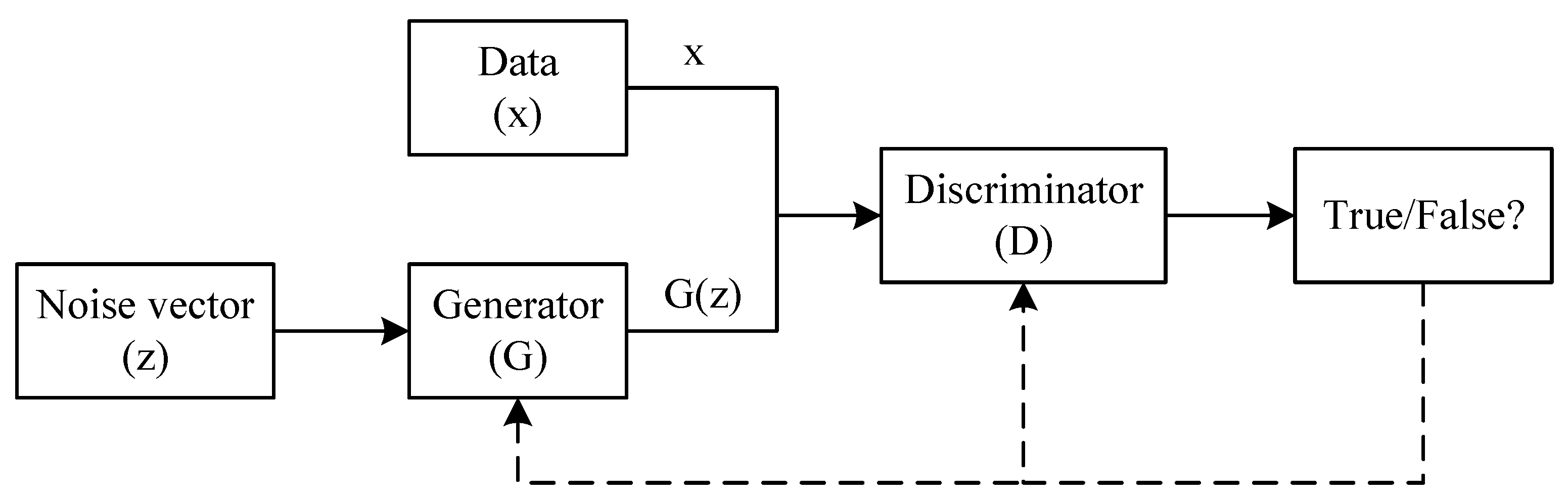
2.1. GAN

The GAN [21] is an unsupervised deep learning model that can learn the distribution of samples and generate new sample data without relying on prior assumptions. The typical structure is shown in Figure 1. GAN optimizes generator and discriminator by alternate iteration. G(z) tries to satisfy the probability distribution of the real sample x, while discriminator D tries to distinguish between x and G(z). Through continuous confrontation training, the generator and discriminator finally reach Nash equilibrium.

For the original GAN, Jensen-Shannon (JS) divergence is used to measure the gap between the generated sample and the real sample. In the process of seeking Nash equilibrium, model collapse or gradient disappearance will lead to the non-convergence of the neural network. In WGAN, JS distance is replaced by Wasserstein distance [22]. The replacement of loss function brings the following advantages: the problem of unstable GAN training is completely solved, and it is no longer necessary to carefully balance the training degree of generator and discriminator; the problem of collapse mode is solved to ensure the diversity of generated samples; the design of network architecture becomes simple, which is conducive to the combination with CNN to realize image generation. The Wasserstein distance is defined as:

$$W\left(P_r,P_g\right)=\underset{\delta \in \mathsf{\Pi }\left(P_r,P_g\right)}{inf}{E}_{(x,y)\sim \delta }[\parallel x-y\parallel ]$$

(1)

where $P_r$ and $P_g$ represent the data distribution of the real sample and the generated sample; $\mathsf{\Pi }\left(P_r,P_g\right)$ represents the set of joint probability distribution $\delta$ with $P_r$ and $P_g$ as the marginal distribution; $W\left(P_r,P_g\right)$ represents the distance of x to y required to fit $P_g$ to $P_r$. The Kantorovich-Rubinstein dual form of $W\left(P_r,P_g\right)$ is adopted in the actual calculation, as shown in Equation (2).

$$W\left(P_r,P_g\right)=\underset{{\parallel f\parallel }_L\le 1}{sup}{E}_{x\sim P_r}\left[f\left(x\right)\right]-E_{x\sim P_g}\left[f\left(x\right)\right]$$

(2)

${\parallel f\parallel }_L\le 1$ means that $f\left(x\right)$ satisfies the 1-Lipschitz condition. WGAN uses weight clipping to limit the weight of the discriminator network to a fixed range to approximate the Wasserstein distance. The generator network is optimized to minimize the Wasserstein distance, thereby effectively narrowing the distribution of generated samples and real samples. The loss functions of generator and discriminator are defined as ${Loss}_G$ and ${Loss}_D$, respectively, as shown in Equations (3) and (4).

$${Loss}_G=-E_{x\sim P_g}\left[D\left(x\right)\right]$$

(3)

$${Loss}_D=E_{x\sim P_g}\left[D\left(x\right)\right]-E_{x\sim P_r}\left[D\left(x\right)\right]$$

(4)

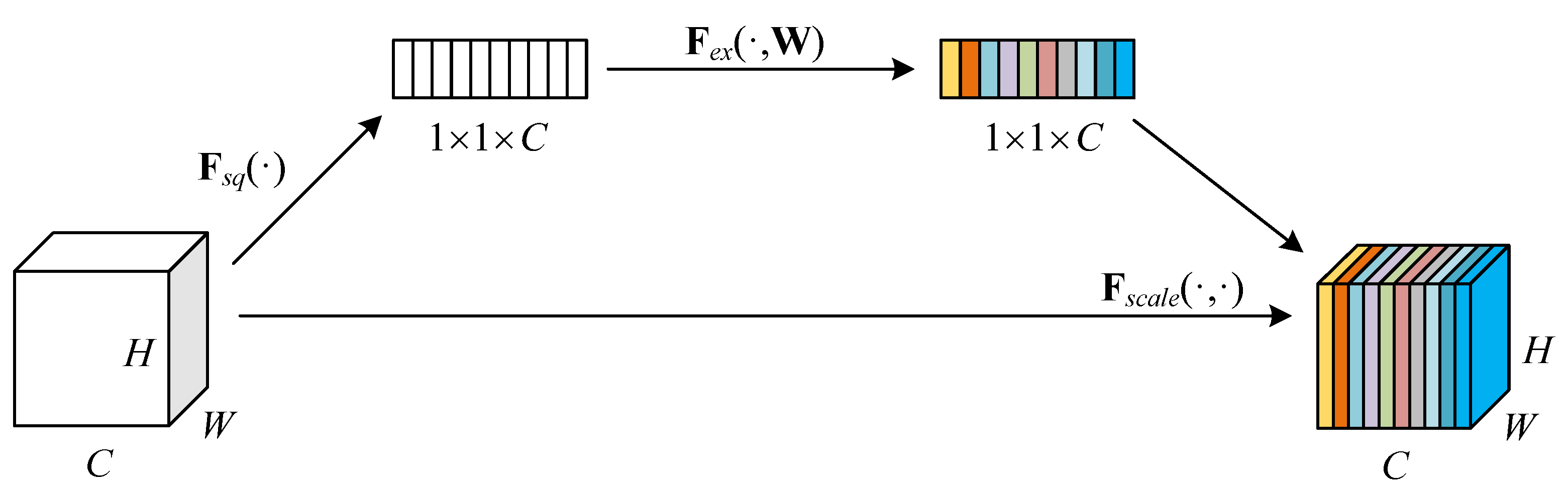
2.2. Squeeze-and-Excitation Block

Squeeze-and-excitation block (SE block) [23] is shown in Figure 2. By learning the weights of the feature maps, effective channels are amplified and invalid or less effective channels are suppressed, thereby achieving the purpose of improving the accuracy of the model.

The height, width, and channel number of the input feature map ${\mathit{u}}_c$ are H, W and C, respectively. Through squeeze and global average pooling algorithm, the output feature map is transformed from $H\times W\times C$ to $1\times 1\times C$, as shown in Equation (5).

$$z_c={\mathit{F}}_{sq}\left({\mathit{u}}_c\right)=\frac{1}{W\times H}\sum _{i=1}^W\sum _{j=1}^H{u}_c(i,j)$$

(5)

where $Z_c$ represents the output feature map, and $(i,j)$ represents the coordinate position on the feature map. Through excitation, two fully connected layers ${\mathbf{W}}_1$ and ${\mathbf{W}}_2$ are utilised to merge the information of the channels. The dimension of ${\mathbf{W}}_1$ is set to $1\times 1\times \frac{C}{r}$ to reduce the computational effort, where r represents reduction ratio. The dimension of ${\mathbf{W}}_2$ is restored to $1\times 1\times C$. Finally, the channel weight $\mathit{v}$ is obtained, as shown in Equation (6).

$$\mathit{v}={\mathit{F}}_{ex}\left(z_c,{\mathbf{W}}_i\right)=\delta \left({\mathbf{W}}_2\sigma \left({\mathbf{W}}_1{z}_c\right)\right)$$

(6)

where $\sigma$ is ReLU activation function and $\delta$ is Sigmoid activation function. The adjustment parameters between the channels are multiplied by the original feature map to realize the recalibration, as shown in Equation (7).

$${\mathit{X}}_c={\mathit{F}}_{\mathrm{scale}}\left({\mathit{u}}_c,v_c\right)={\mathit{u}}_c{v}_c$$

(7)

where $v_c$ represents the weight parameter of the c th feature map, ${\mathit{X}}_c$ represents the adjusted feature map.

2.3. Feature Visualization

The features extracted by deep convolutional networks are highly abstract, which is difficult to visually display the information of interest. With the deepening of research, Gradient-weighted Class Activation Mapping (Grad-CAM) [24] has gradually become a powerful visualization tool. Grad-CAM is able to present the features of most interest to the model in the form of a heat map, which calculates the weights of the features primarily by employing a global average of the gradients.

The gradient of the model score for category C is first calculated for a particular convolutional layer, while for the gradient information obtained by the above process, the importance weights of the neurons are obtained by averaging the pixel values over each channel dimension, as shown in Equation (8).

$${\alpha }_i^{\mathrm{c}}=\frac{1}{Z}\sum _{k=1}^{c_1}\sum _{j=1}^{c_2}\frac{\partial S_c}{\partial A_{kj}^i}$$

(8)

where Z is the number of pixels in the feature map, $S_c$ is the classification score for category C. $c_1\times c_2$ represents the dimension of the feature map. $A_{kj}^i$ represents the pixel value of the k th row and j th column of the i th feature map, and ${\alpha }_i^{\mathrm{c}}$ is the weight of class C relative to the i th channel of the feature map output by the last convolution layer. The weighted average is executed and then passed through the ReLU function to obtain the Grad-CAM feature map. The formula is shown in Equation (9).

$$L^c=ReLU\left(\sum _i{\alpha }_i^c{A}^i\right)$$

(9)

where $L^c$ represents the activated heat map of class C and $A^i$ represents the i th feature map.

2.4. Our Methods

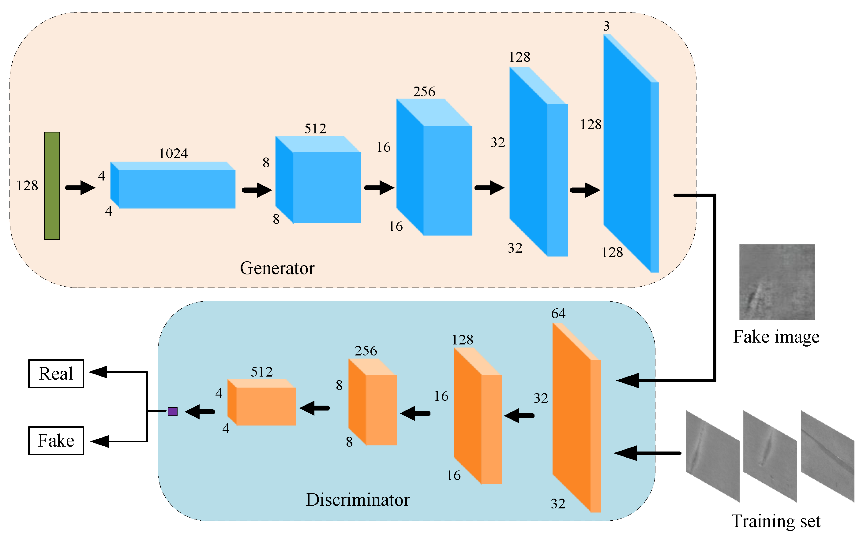
2.4.1. A Novel WGAN Model

A novel WGAN model is proposed and used for data augmentation of strip steel surface defect images, as shown in Figure 3. The implementation of the discriminator is similar to that of a general CNN [25]. The activation functions between discriminator convolutional layers all use LeakyReLU. It should be noted that the Sigmoid function is not used in the last layer. The input of the generator is a 128-dimensional random noise vector conforming to the standard normal distribution. Between levels, batch normalization is used to accelerate convergence and slow down overfitting. The tanh function is used to activate the output layer, and the ReLU function is used to activate the remaining layers. With the transposed convolution, the number of channels gradually decreases and the dimensions continue to increase, so that the three-channel pseudo image is finally generated.

By modifying the dimension of the last layer of the generator to 128 × 128, the generated image can directly maintain the same size as the original image, which facilitates subsequent classification research.

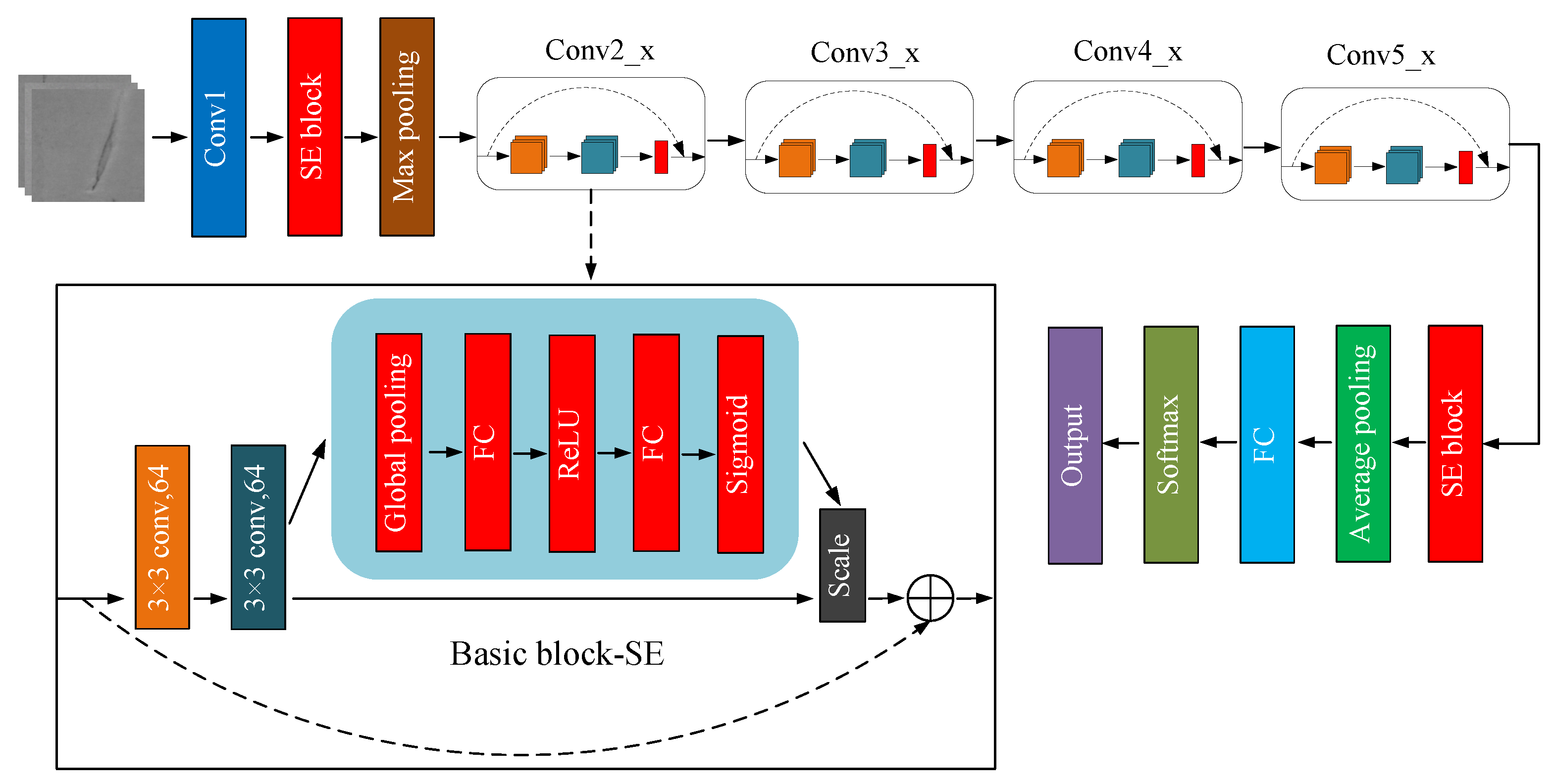
2.4.2. Multi-SE-ResNet34 Model

Based on current experience, increasing the depth of network can improve network performance. However, the degradation phenomenon that occurs during the back propagation of the error gradient may cause difficulties in network convergence. In the deep residual network (ResNet) proposed by He et al. [26] in 2015, the addition of identity mapping solves the problem that deep network models are difficult to train. In the last few years, ResNet has been widely used in various classification tasks [27,28,29,30] with strong capabilities. On this basis, a Multi-SE-ResNet34 model combined with the attention mechanism is proposed, and the structure is shown in Figure 4.

Multi-SE-ResNet34 is an improvement of ResNet34, which is mainly composed of four different types of Basic block-SE modules. This module embeds SE block in each residual unit. From Conv2_x to Conv5_x, there are 3, 4, 6, and 3 Basic block-SEs, and all Basic block-SEs use a 3 × 3 convolution kernel. As the depth of the model increases, the number of convolution kernels keeps consistent with ResNet34. Moreover, two additional SE blocks are added outside the residual structure, which are located after the first convolutional layer and before the average pooling layer. Due to the attention mechanism, the performance of the proposed model is better than that of the basic ResNet34, which will give support in the discussion.

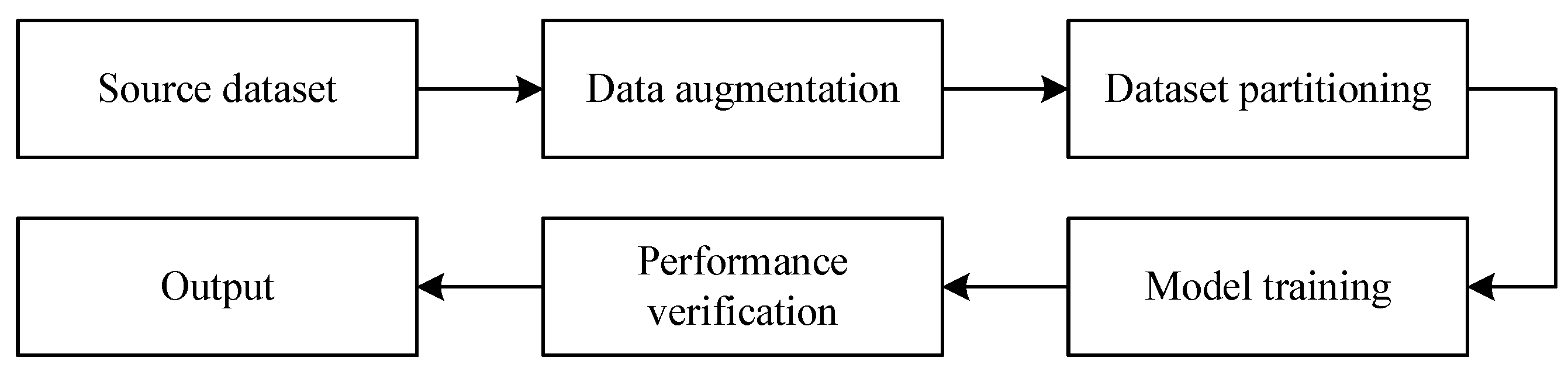
2.4.3. Overall Process

The overall process of our methods is shown in Figure 5. First, the WGAN model is constructed for data augmentation. The generated image and the original image together form a new data set. Second, the enhanced data set is divided into training set, validation set and test set. The function of the test set lies in the evaluation of performance and the output of classification results.

3. Experiments and Results

The experiment is based on the following hardware and software environment: Windows10 operating system of Microsoft, Intel(R) Core (TM) i7-11800H CPU, NVIDIA GeForce RTX 3060 Laptop GPU, NVIDIA CUDA-11.1.1 and cuDNN-11.2, Pytorch v1.8.0 deep learning framework.

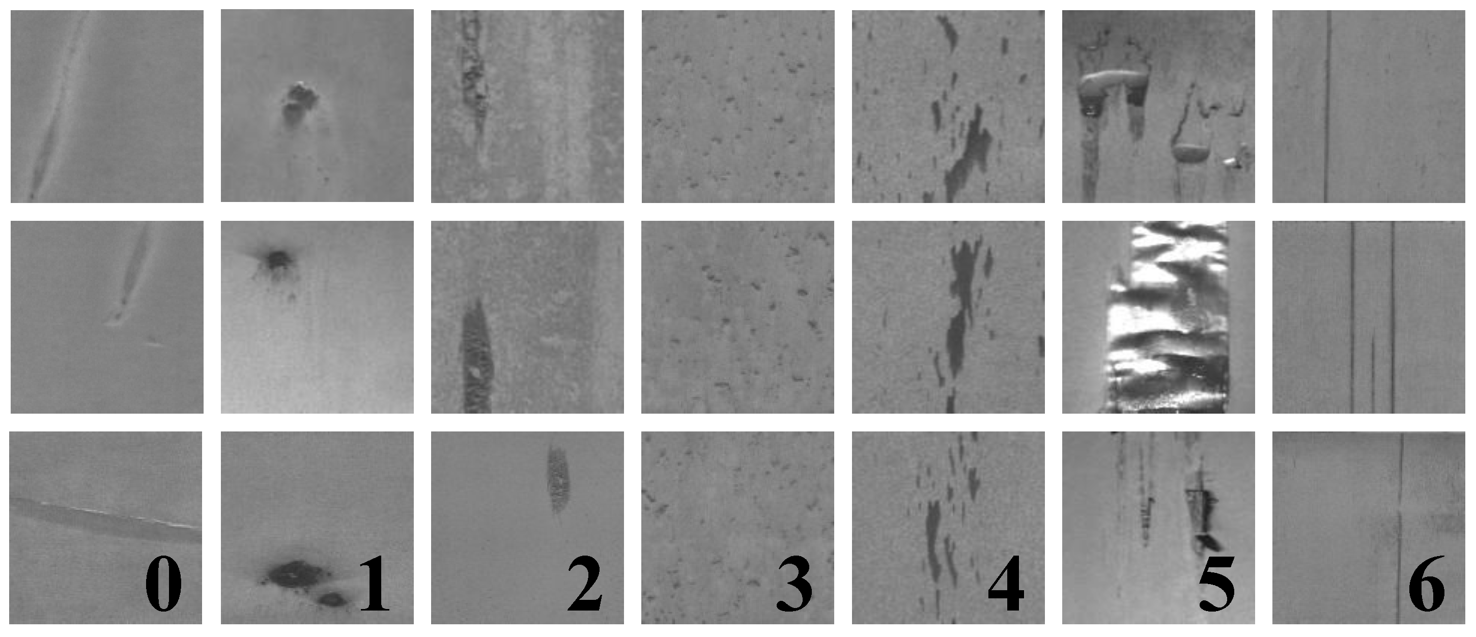
3.1. Introduction to the Data Set

The X-SDD data set [31] contains 1360 strip steel surface defect images in 7 categories. The size of each image is 128 × 128 pixels, and the format is 3-channel JPG. Several samples of each defect are shown in Figure 6. For the convenience of description, the 7 types of images are marked with tags of 0, 1, 2, 3, 4, 5, and 6.

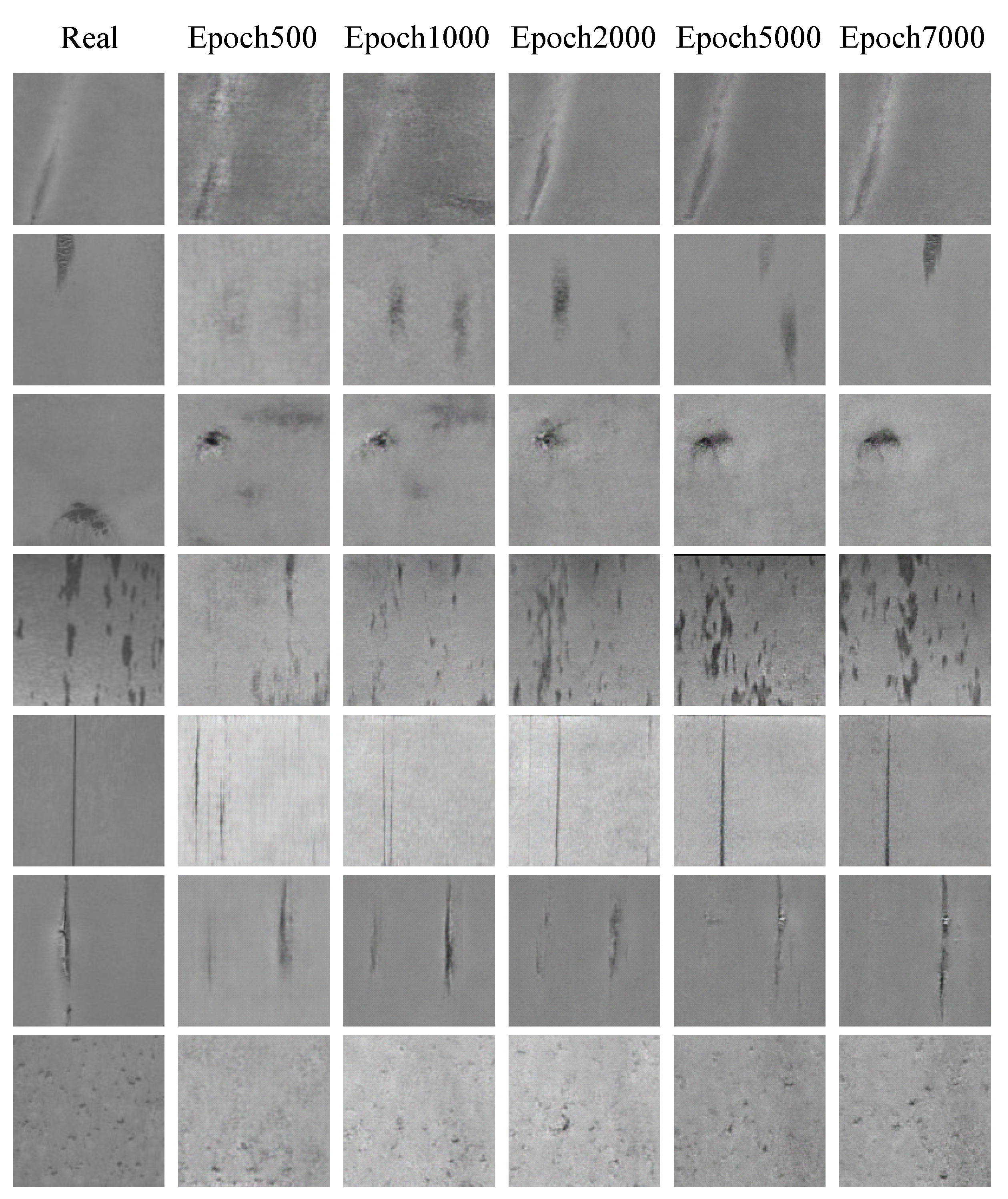
3.2. Image Generation

After training the discriminator five times, the generator is trained once. Both the generation network and the discriminant network use RMSProp algorithm to update parameters, including learning rate of 0.00005, clipping parameter of 0.01, batch size of 32, and epoch of 7000. The strip steel surface defect images generated by the proposed WGAN model at different stages are shown in Figure 7.

It can be seen that when the number of iterations is 500, the generated image contains more meaningless information. At this point, the discriminator can easily distinguish false samples. When the number of iterations reaches 2000, the generator gradually learns the data distribution of the real image. At this point, the generated image has a rough outline of the defect. However, a lot of texture information is lost and blurred visually. After 7000 epochs, the generated image is close to the real image, with clear outline and distribution of defects. Unlike linear transformations such as rotation and scaling, the generated image guarantees the diversity of features. The total number of samples increases from 1360 to 3773 after data augmentation. The specific number of each type of defect is shown in

Table 1. Number of defective images.

Category	0	1	2	3	4	5	6
Original	203	122	63	203	397	238	134
Enhanced	589	517	498	530	595	488	556

.

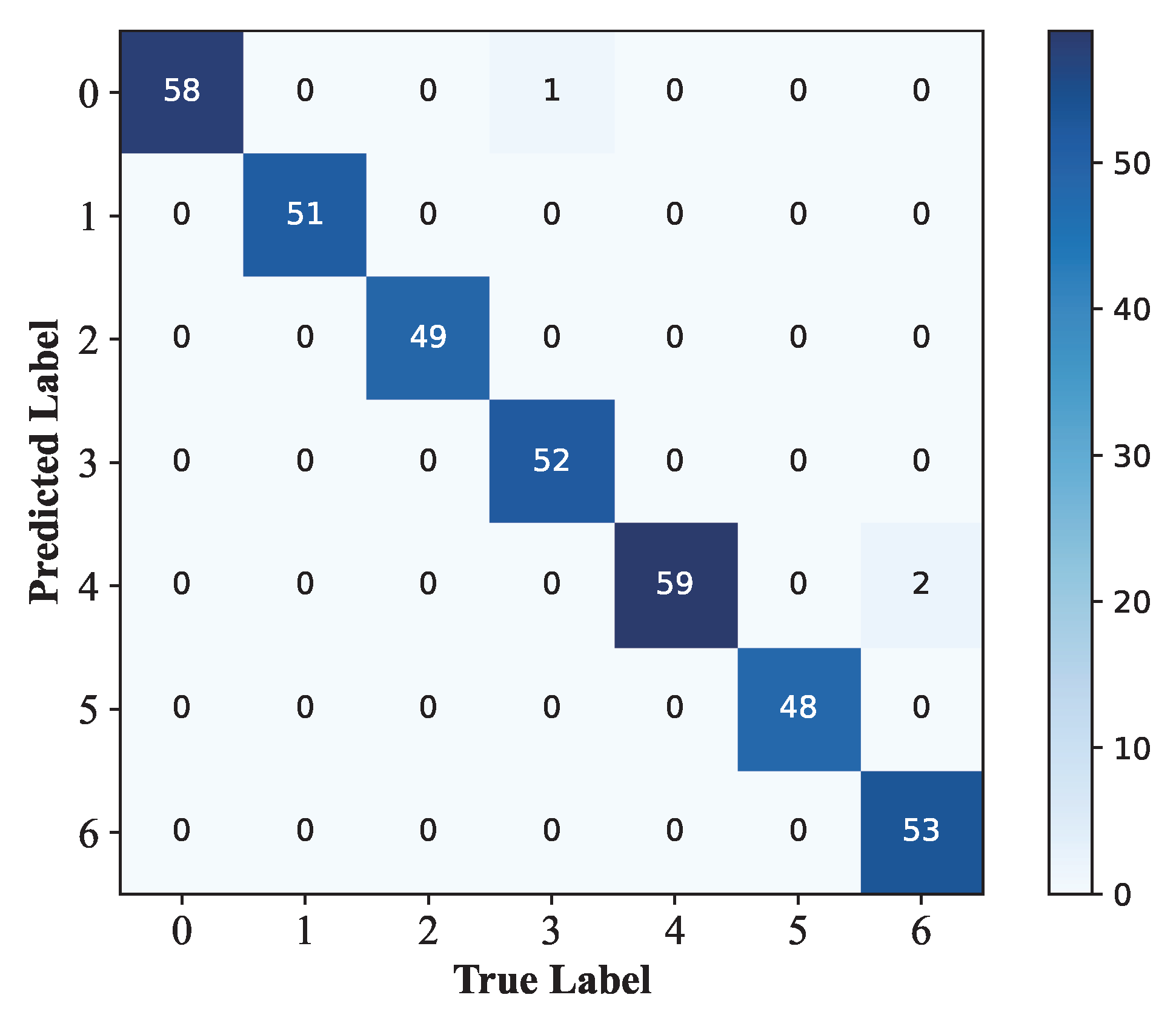
3.3. Defect Classification

In the classification experiment, the data set after data augmentation is divided. First, 10% sample is randomly sampled to form a testing set. Then, the remaining images are divided into training set and validation set with the ratio of 8:2. The number of images in the training set, validation set, and testing set are 2722, 678 and 373, respectively. The input image of Multi-SE-ResNet34 is set to a size of 224 × 224 and normalized with batch size of 16. The reduction ratio of SE block is set to 16. Stochastic gradient descent with momentum is used for parameter update with the momentum factor of 0.9 and initial learning rate of 0.001. The learning rate is reduced to one-tenth of the original after 20 epochs. Moreover, L2 regularization is used to prevent overfitting, with the weight decay coefficient of 0.0001. Figure 8 shows the loss and accuracy curves. During the first 10 iterations, the loss drops rapidly and the accuracy rises. As the learning rate decreases, the model tends to stabilize. The loss approaches 0 after the iteration is completed.

In the test set, the classification performance of the model is evaluated. We chose indicators such as Accuracy, Macro-Precision, Macro-Recall and Macro-F1. The above indicators are given by Equations (10)–(13).

$$\mathit{Accuracy}=\frac{n_{-}\mathit{correct}}{n_{-}\mathit{total}}$$

(10)

$$\mathit{Macro}-\mathit{Precision}=\frac{1}{N}\sum _{i=1}^N\frac{T{P}_i}{T{P}_i+F{P}_i}$$

(11)

$$\mathit{Macro}-\mathit{Recall}=\frac{1}{N}\sum _{i=1}^N\frac{T{P}_i}{T{P}_i+F{N}_i}$$

(12)

$$\mathit{Macro}-{\mathit{F}}_{\mathit{1}}=\frac{1}{N}\sum _{i=1}^N\frac{2\times P_i\times R_i}{P_i+R_i}$$

(13)

where, $n_{-}\mathit{correct}$ is the number of samples correctly classified by the model; $n_{-}\mathit{total}$ is the total number of samples; $TP$, $FP$, $TN$ and $FN$ represent true positive, false positive, true negative, and false negative, respectively. N is the number of defect types. P and R represent precision and recall.

The classification results are shown in

Table 2. Classification results.

Accuracy (%)	Macro-Precision (%)	Macro-Recall (%)	Macro-F1 (%)
99.20	99.29	99.21	99.24

. The generated confusion matrix is shown in Figure 9. The accuracy of Multi-SE-ResNet34 is 99.20%, demonstrating the robustness of our method for feature recognition of a wide range of strip steel surface defects. According to the confusion matrix, defects 0, 1, 2, 4, and 5 can be identified 100%. The accuracy of defect 6 is relatively low, and two images are classified as defect 4. Some of the defects 4 have a slender distribution, which is similar to that of defects 6, which leads to an increase in the difficulty of classification. On the whole, our method can accurately classify 7 kinds of strip steel surface defects.

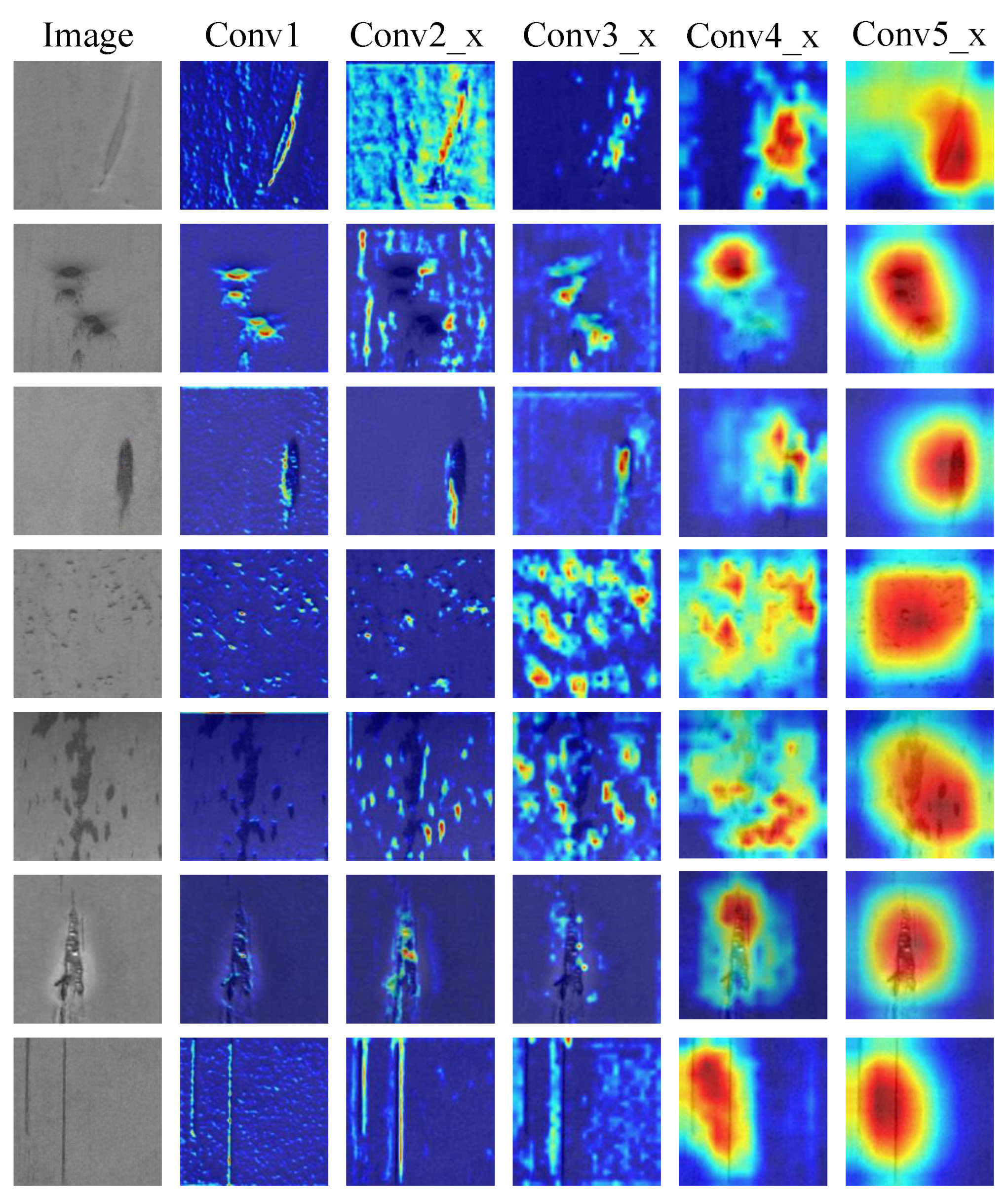
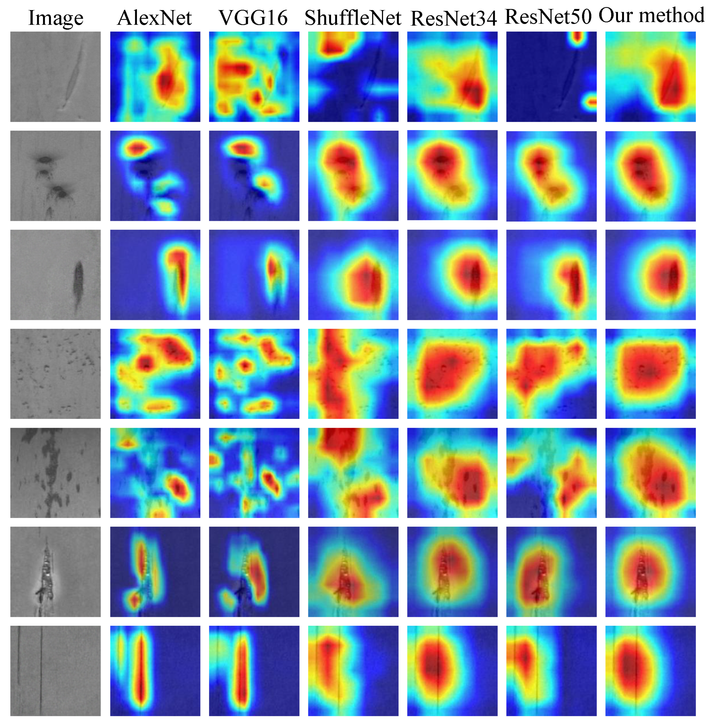
3.4. Grad-CAM Visualization

Seven defect images are randomly selected and used to generate visual heat maps of each layer of Multi-SE-ResNet34, as shown in Figure 10. It can be clearly seen that the number of layers in the network at the end of Conv1 is very shallow and the model extracts few features. As the number of convolutional layers increases, the feature recognition capability is enhanced, and the features learned by the model becomes rich at the end of Conv4_x, but still insufficient to cover the whole defect. The model extracts enough features at the end of Conv5_x, and at the same time, the area of interest is exactly where the defects are located due to the addition of the attention module. It can be concluded that our model has excellent recognition performance for all seven strip surface defects features.

4. Discussions

4.1. The Impact of Sample Size on Classification Results

Classification using Multi-SE-ResNet34 on the source dataset yielded an accuracy of 93.98%. Nevertheless, the accuracy is improved by 5.22% after data augmentation, i.e., 99.20%, which shows the classification performance is closely related to the number of samples. Although studies have pointed this out [32,33], there are few complete identification cases. Therefore, our method generates realistic images and improves recognition accuracy, providing an effective solution for the small sample size of strip steel surface defect images.

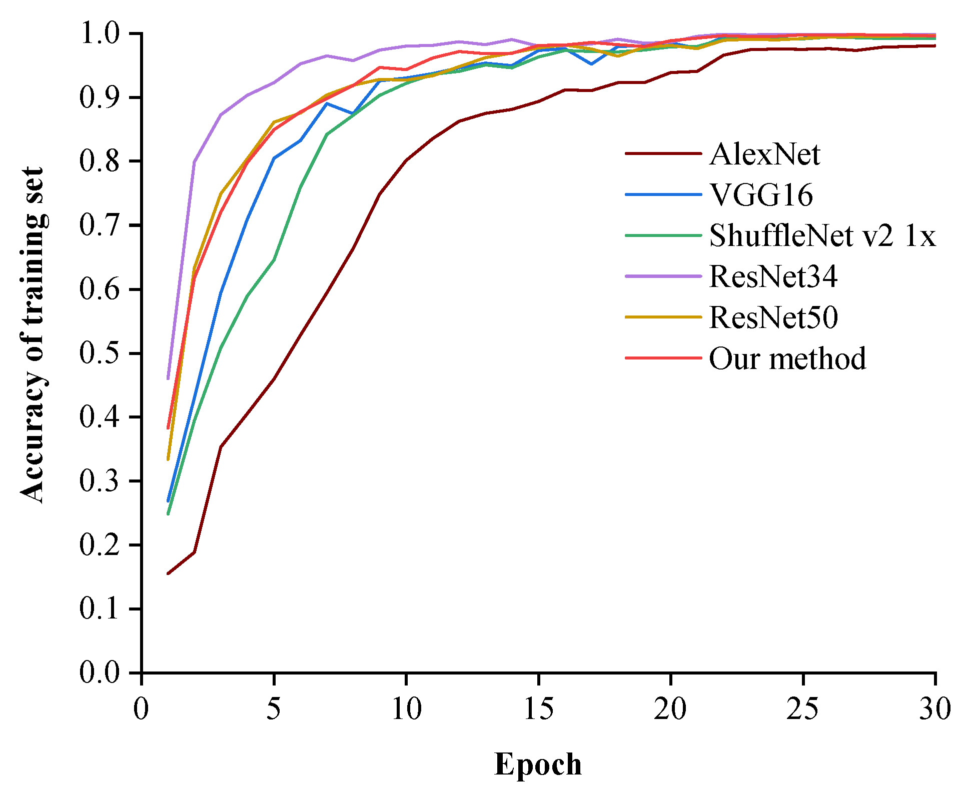
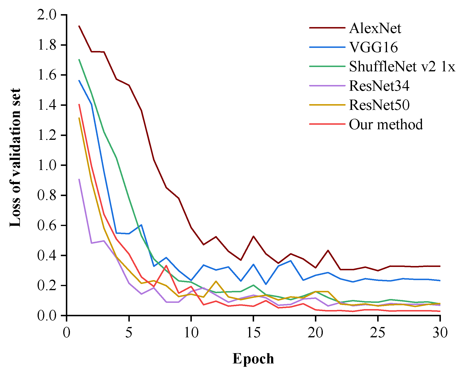
4.2. Comparison with Other Models

In order to further verify the remarkable performance of our method, the classical models of AlexNet [34], VGG16 [35], ShuffleNet v2 1× [36], ResNet34 and ResNet50 [26] are selected for comparison using the enhanced dataset with the same hyperparameters. The classification results of each model on the test set are shown in

Table 3. Comparison of different models.

Model	Accuracy (%)	Macro-Precision (%)	Macro-Recall (%)	Macro-F1 (%)
AlexNet	92.49	92.82	92.15	92.19
VGG16	94.64	95.06	94.30	94.45
ShuffleNet v2 1×	97.32	97.38	97.26	97.30
ResNet34	98.66	98.68	98.59	98.61
ResNet50	97.86	97.88	97.72	97.77
Our method	99.20	99.29	99.21	99.24

. It can be seen that our method obtains the highest accuracy rate, which is 6.71%, 4.56%, 1.88%, 0.54% and 1.34% higher than AlexNet, VGG16, ShuffleNet v2 1×, ResNet34, and ResNet50, respectively. At the same time, our model is also optimal on three other evaluation indicators.

Figure 11 shows the accuracy curves for the training set of each model. It can be seen that after 10 iterations of training, the accuracy of all models except AlexNet exceeds 90%, with AlexNet having the lowest accuracy due to its shallow network layers. The accuracy of each model increases over the first 20 epochs, reaching its maximum value and stabilising after the learning rate is reduced; after the completion of iterations, all models except AlexNet obtain an accuracy of over 99.41%. In terms of convergence speed, AlexNet is the slowest, in contrast to ResNet34. The lower convergence speed of ShuffleNet than VGG16 is attributed to the reduction in the number of parameters due to the lightweight implementation, where the recognition ability is diminished. Our method achieves a satisfactory convergence rate, comparable to that of ResNet50, but lower than that of ResNet34. One possible reason is that the number of parameters increased with the addition of multiple SE blocks, and fewer iterations are not sufficient to extract enough features. However, our method has the highest accuracy and achieves a balance between recognition effectiveness and number of parameters, which can be considered more advantageous.

The loss curves in the validation set of each model are shown in Figure 12. It can be seen that both AlexNet and VGG16 have large fluctuations and are less stable. The curve of ShuffleNet is the smoothest. There are several fluctuations in ResNet34 and ResNet50 where stability is compromised. The curve of our method is relatively smooth overall, with only a few minor fluctuations that do not affect the decreasing course of loss. All models converge after 20 iterations. At the end of training, the loss of our method is the lowest, maintaining at 0.029. On the whole, a stable training process, the lowest loss value and the highest accuracy have been obtained, therefore our method is optimal for the classification of strip surface defects.

4.3. Influence of Attention Mechanism on Feature Extraction

Heat maps of the strip surface defect features extracted by the last convolutional layer of each model are generated to explore the influence of attention mechanism on feature extraction, as shown in Figure 13. It can be seen that AlexNet struggles to extract features effectively due to its shallow network layers. VGG16 simply stacks convolutional layers, with no obvious improvement in feature extraction capability compared to AlexNet. The features extracted by ShuffleNet increased but with a large amount of useless information. In particular, despite the relatively deep depth of the ResNet50 network, it failed to accurately extract features of defect 0 and defect 4. The performance of ResNet34 is outstanding with an excellent feature extraction capability. Nevertheless, in comparison, our method not only extracts sufficient features, but also reduces invalid information in the background and locates feature regions more precisely, which verifies the comparison results in Section 4.2. In other words, benefiting from the attention mechanism, our method is more calibrated in terms of feature extraction.

5. Conclusions

• For the small sample size of strip steel surface defect images, a novel WGAN model is proposed and used for data augmentation. The generated image has a resolution of 128 × 128 and the appearance is close to the real image, which can be directly used to expand the original data set.
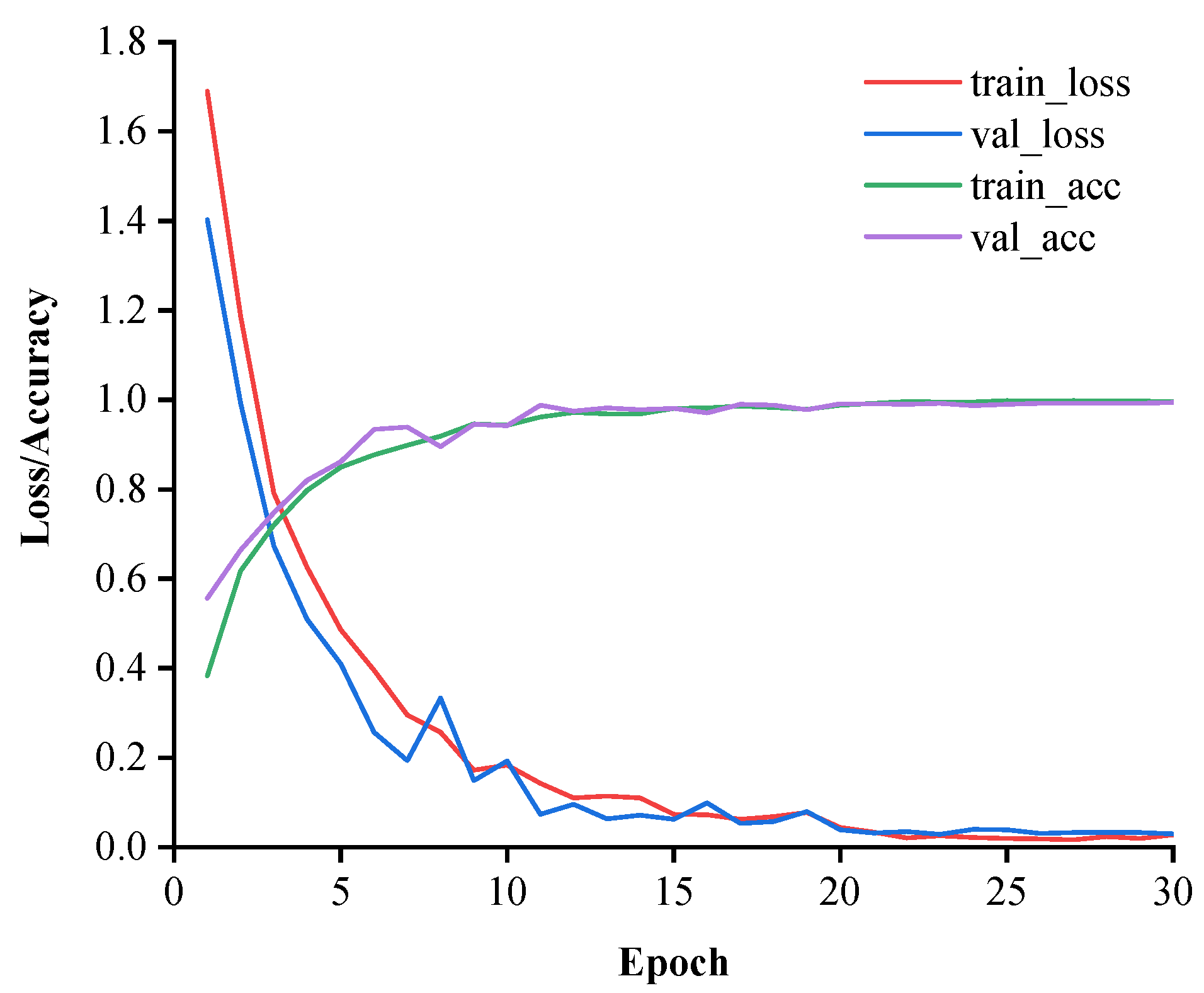
• A Multi-SE-ResNet34 model combining channel attention mechanism is proposed and used for defect classification with 99.20% accuracy. In addition, Multi-SE-ResNet34 outperforms the other models in terms of Macro-Precision, Macro-Recall and Macro-F1. The training process of Multi-SE-ResNet34 is stable, and the validation set loss tends to 0. Furthermore, there is no over-fitting phenomenon.
• The Grad-CAM method is used to visually analyze the defect features extracted by different models, which shows that the attention mechanism can make the model pay attention to more valuable information and improve the classification accuracy. The advantages of our method are further demonstrated.

In the future, we have the expectation of combining spatial attention and channel attention to further improve the recognition rate and realize the lightweight of the network.

References

- Tang, W.; Liong, S.; Chen, C.; Tsai, M.; Hsieh, P.; Tsai, Y.; Chen, S.; Wang, K. Design of Multi-Receptive Field Fusion-Based Network for Surface Defect Inspection on Hot-Rolled Steel Strip Using Lightweight Dataset. Appl. Sci. 2021, 11, 9473. [Google Scholar] [CrossRef]
- Sun, J.; Peng, W.; Ding, J.; Li, X.; Zhang, D. Key intelligent technology of steel strip production through process. Metals 2018, 8, 597. [Google Scholar] [CrossRef] [Green Version]
- Feng, X.; Gao, X.; Luo, L. A ResNet50-Based Method for Classifying Surface Defects in Hot-Rolled Strip Steel. Mathematics 2021, 9, 2359. [Google Scholar] [CrossRef]
- Zhang, J.; Kang, X.; Ni, H.; Ren, F. Surface defect detection of steel strips based on classification priority YOLOv3-dense network. Ironmak. Steelmak. 2021, 48, 547–558. [Google Scholar] [CrossRef]
- Kim, C.; Choi, S.; Kim, G.; Joo, W. Classification of surface defect on steel strip by KNN classifier. J. Korean Soc. Precis. Eng. 2006, 23, 80–88. [Google Scholar]
- Karthikeyan, S.; Pravin, M.C.; Sathyabama, B.; Mareeswari, M. DWT Based LCP Features for the Classification of Steel Surface Defects in SEM Images with KNN Classifier. Aust. J. Basic Appl. Sci. 2016, 10. Available online: https://ssrn.com/abstract=2792637 (accessed on 17 April 2021).
- Martins, L.A.; Pádua, F.L.; Almeida, P.E. Automatic detection of surface defects on rolled steel using computer vision and artificial neural networks. In Proceedings of the IECON 2010-36th Annual Conference on IEEE Industrial Electronics Society, Glendale, AZ, USA, 7–10 November 2010; pp. 1081–1086. [Google Scholar]
- Bulnes, F.G.; García, D.F.; De la Calle, F.J.; Usamentiaga, R.; Molleda, J. A non-invasive technique for online defect detection on steel strip surfaces. J. Nondestruct. Eval. 2016, 35, 1–18. [Google Scholar] [CrossRef]
- Hu, H.; Liu, Y.; Liu, M.; Nie, L. Surface defect classification in large-scale strip steel image collection via hybrid chromosome genetic algorithm. Neurocomputing 2016, 181, 86–95. [Google Scholar] [CrossRef]
- Jiang, M.; Li, G.; Xie, L.; Xiao, M.; Yi, L. Adaptive classifier for steel strip surface defects. J. Phys. 2017, 787, 012019. [Google Scholar] [CrossRef]
- Zaghdoudi, R.; Seridi, H.; Ziani, S. Binary Gabor pattern (BGP) descriptor and principal component analysis (PCA) for steel surface defects classification. In Proceedings of the 2020 International Conference on Advanced Aspects of Software Engineering (ICAASE), Constantine, Algeria, 28–30 November 2020; pp. 1–7. [Google Scholar]
- Yi, L.; Li, G.; Jiang, M. An end-to-end steel strip surface defects recognition system based on convolutional neural networks. Steel Res. Int. 2017, 88, 1600068. [Google Scholar] [CrossRef]
- Fu, G.; Sun, P.; Zhu, W.; Yang, J.; Cao, Y.; Yang, M.Y.; Cao, Y. A deep-learning-based approach for fast and robust steel surface defects classification. Opt. Laser Eng. 2019, 121, 397–405. [Google Scholar] [CrossRef]
- Liu, Y.; Geng, J.; Su, Z.; Zhang, W.; Li, J. Real-time classification of steel strip surface defects based on deep CNNs. In Proceedings of the 2018 Chinese Intelligent Systems Conference, Wenzhou, China, 10–13 March 2019; pp. 257–266. [Google Scholar]
- Konovalenko, I.; Maruschak, P.; Brezinová, J.; Viňáš, J.; Brezina, J. Steel surface defect classification using deep residual neural network. Metals 2020, 10, 846. [Google Scholar] [CrossRef]
- Wang, W.; Lu, K.; Wu, Z.; Long, H.; Zhang, J.; Chen, P.; Wang, B. Surface Defects Classification of Hot Rolled Strip Based on Improved Convolutional Neural Network. ISIJ Int. 2021, 61, 1579–1583. [Google Scholar] [CrossRef]
- Wan, X.; Zhang, X.; Liu, L. An Improved VGG19 Transfer Learning Strip Steel Surface Defect Recognition Deep Neural Network Based on Few Samples and Imbalanced Datasets. Appl. Sci. 2021, 11, 2606. [Google Scholar] [CrossRef]
- Xu, L.; Tian, G.; Zhang, L.; Zheng, X. Research of Surface Defect Detection Method of Hot Rolled Strip Steel Based on Generative Adversarial Network. In Proceedings of the 2019 Chinese Automation Congress (CAC), Hangzhou, China, 22–24 November 2019; pp. 401–404. [Google Scholar]
- Cao, Y.; Xu, J.; Lin, S.; Wei, F.; Hu, H. Gcnet: Non-local networks meet squeeze-excitation networks and beyond. In Proceedings of the IEEE/CVF International Conference on Computer Vision Workshops, Seoul, Korea, 27–28 October 2019. [Google Scholar]
- Wang, F.; Jiang, M.; Qian, C.; Yang, S.; Li, C.; Zhang, H.; Wang, X.; Tang, X. Residual attention network for image classification. In Proceedings of the IEEE Conference on Computer Vision and Pattern Recognition, Honolulu, HI, USA, 21–26 July 2017; pp. 3156–3164. [Google Scholar]
- Goodfellow, I.J.; Pouget-Abadie, J.; Mirza, M.; Xu, B.; Warde-Farley, D.; Ozair, S.; Courville, A.; Bengio, Y. Generative adversarial networks. Adv. Neural Inf. Process. Syst. 2014, 3, 2672–2680. [Google Scholar] [CrossRef]
- Jiao, Z.; Ren, F. WRGAN: Improvement of RelGAN with Wasserstein Loss for Text Generation. Electronics 2021, 10, 275. [Google Scholar] [CrossRef]
- Hu, J.; Shen, L.; Sun, G. Squeeze-and-excitation networks. In Proceedings of the IEEE Conference on Computer Vision and Pattern Recognition, Salt Lake City, UT, USA, 18–23 June 2018; pp. 7132–7141. [Google Scholar]
- Selvaraju, R.R.; Cogswell, M.; Das, A.; Vedantam, R.; Parikh, D.; Batra, D. Grad-cam: Visual explanations from deep networks via gradient-based localization. In Proceedings of the IEEE International Conference on Computer Vision, Venice, Italy, 22–29 October 2017; pp. 618–626. [Google Scholar]
- Wang, K.; Zhang, J.; Ni, H.; Ren, F. Thermal Defect Detection for Substation Equipment Based on Infrared Image Using Convolutional Neural Network. Electronics 2021, 10, 1986. [Google Scholar] [CrossRef]
- He, K.; Zhang, X.; Ren, S.; Sun, J. Deep residual learning for image recognition. In Proceedings of the IEEE Conference on Computer Vision and Pattern Recognition, Las Vegas, NV, USA, 27–30 June 2016; pp. 770–778. [Google Scholar]
- Li, B.; He, Y. An improved ResNet based on the adjustable shortcut connections. IEEE Access 2018, 6, 18967–18974. [Google Scholar] [CrossRef]
- Ren, F.; Liu, W.; Wu, G. Feature reuse residual networks for insect pest recognition. IEEE Access 2019, 7, 122758–122768. [Google Scholar] [CrossRef]
- Zhang, Y.; Wa, S.; Sun, P.; Wang, Y. Pear Defect Detection Method Based on ResNet and DCGAN. Information 2021, 12, 397. [Google Scholar] [CrossRef]
- Yang, Y.; Wang, H.; Jiang, D.; Hu, Z. Surface Detection of Solid Wood Defects Based on SSD Improved with ResNet. Forests 2021, 12, 1419. [Google Scholar] [CrossRef]
- Feng, X.; Gao, X.; Luo, L. X-SDD: A New Benchmark for Hot Rolled Steel Strip Surface Defects Detection. Symmetry 2021, 13, 706. [Google Scholar] [CrossRef]
- Antoniou, A.; Storkey, A.; Edwards, H. Augmenting image classifiers using data augmentation generative adversarial networks. In Proceedings of the International Conference on Artificial Neural Networks, Rhodes, Greece, 4–7 October 2018; pp. 594–603. [Google Scholar]
- Liu, K.; Li, A.; Wen, X.; Chen, H.; Yang, P. Steel surface defect detection using GAN and one-class classifier. In Proceedings of the 2019 25th International Conference on Automation and Computing (ICAC), Lancaster, UK, 5–7 September 2019; pp. 1–6. [Google Scholar]
- Krizhevsky, A.; Sutskever, I.; Hinton, G.E. Imagenet classification with deep convolutional neural networks. Adv. Neural Inf. Process. Syst. 2012, 25, 1097–1105. [Google Scholar] [CrossRef]
- Simonyan, K.; Zisserman, A. Very deep convolutional networks for large-scale image recognition. arXiv 2014, arXiv:1409.1556. [Google Scholar]
- Zhang, X.; Zhou, X.; Lin, M.; Sun, J. Shufflenet: An extremely efficient convolutional neural network for mobile devices. In Proceedings of the IEEE Conference on Computer Vision and Pattern Recognition, Salt Lake City, UT, USA, 18–23 June 2018; pp. 6848–6856. [Google Scholar]