
Machine Learning for Predicting Fracture Strain in Sheet Metal Forming


 ,
,  , ,
, ,  and
and 
Abstract
1. Introduction
2. Regression ML Algorithms
2.1. Multilayer Perceptron
2.2. Gaussian Processes
2.3. Support Vector Regression
2.4. Random Forest
2.5. Polynomial Regression
3. Design Procedure
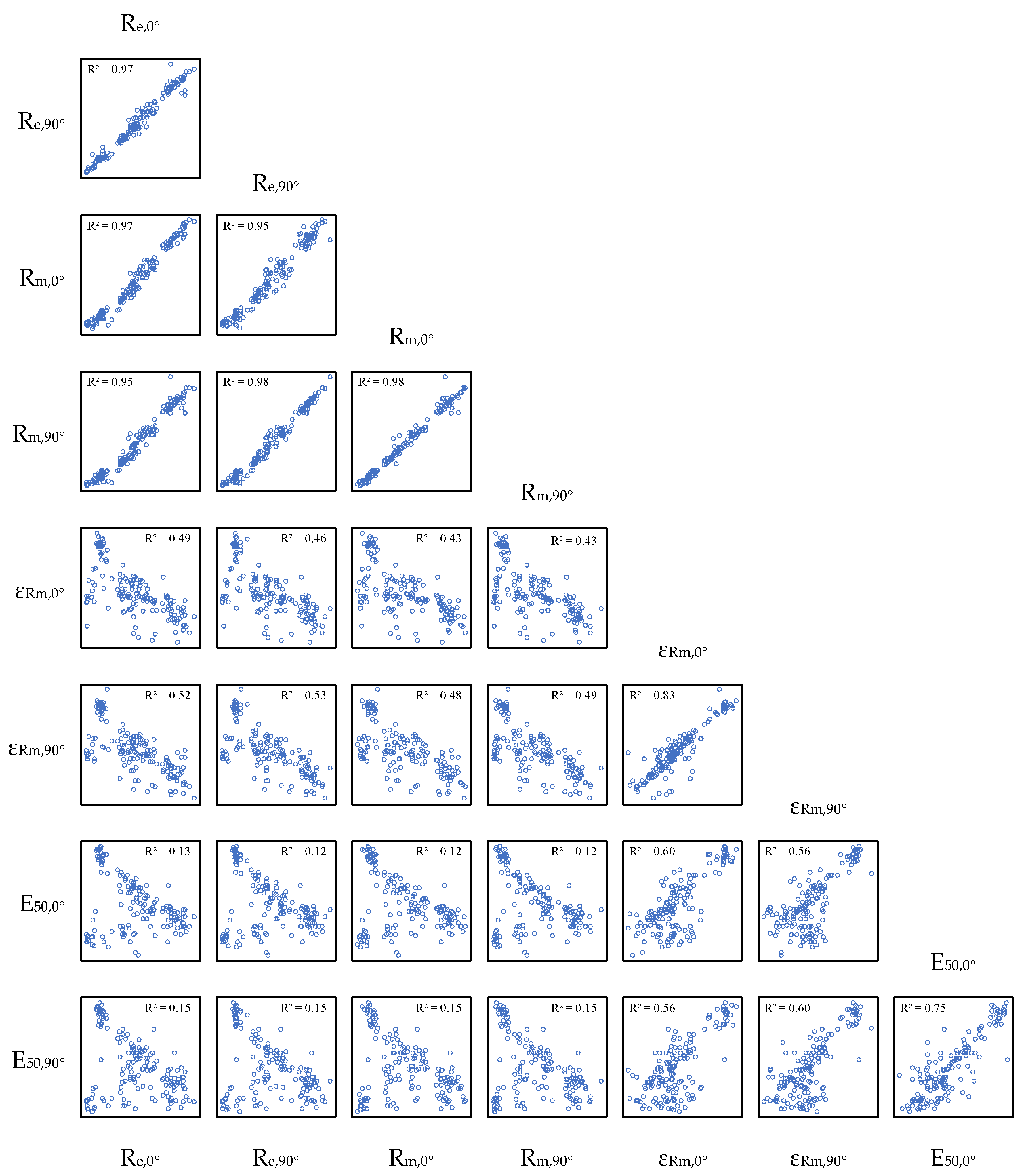
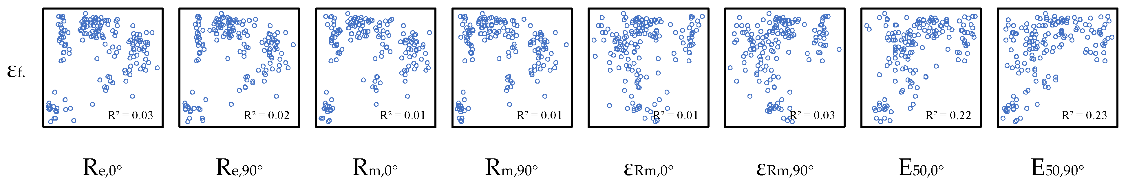
3.1. Dataset
3.2. Model Calibration
3.3. Performance Evaluation
4. Results and Discussion
5. Conclusions
Author Contributions
Funding
Conflicts of Interest
References
- Keeler, S.P.; Backofen, W.A. Plastic instability and fracture in sheets stretched over rigid punches. Trans. Am. Soc. Met. 1963, 56, 25–48. [Google Scholar]
- Goodwin, G.M. Application of strain analysis to sheet metal forming problems in the press shop. SAE Trans. 1968, 77, 380–387. [Google Scholar]
- Stoughton, T.B.; Zhu, X. Review of theoretical models of the strain-based FLD and their relevance to the stress-based FLD. Int. J. Plast. 2004, 20, 1463–1486. [Google Scholar] [CrossRef]
- Graf, A.; Hosford, W. Effect of changing strain paths on forming limit diagrams of AI 2008-T4. Metall. Mater. Trans. A 1993, 24, 1993–2503. [Google Scholar] [CrossRef]
- Abedini, A.; Butcher, C.; Worswick, M.J. Experimental fracture characterisation of an anisotropic magnesium alloy sheet in proportional and non-proportional loading conditions. Int. J. Solids Struct. 2018, 144–145, 1–19. [Google Scholar] [CrossRef]
- McClintock, F.A. A criterion for ductile fracture by the growth of holes. J. Appl. Mech. 1968, 35, 363. [Google Scholar] [CrossRef]
- Lemaitre, J. A Course on Damage Mechanics; Springer: Berlin/Heidelberg, Germany, 1996; ISBN 978-3-540-60980-3. [Google Scholar]
- Wulfinghoff, S.; Fassin, M.; Reese, S. A damage growth criterion for anisotropic damage models motivated from micromechanics. Int. J. Solids Struct. 2017, 121, 21–32. [Google Scholar] [CrossRef]
- Pack, K.; Tancogne-Dejean, T.; Gorji, M.B.; Mohr, D. Hosford-Coulomb ductile failure model for shell elements: Experimental identification and validation for DP980 steel and aluminum 6016-T4. Int. J. Solids. Struct. 2018, 151, 214–232. [Google Scholar] [CrossRef]
- Gurson, A.L. Continuum theory of ductile rupture by void nucleation and growth: Part I—Yield criteria and flow rules for porous ductile media. J. Eng. Mater. Technol. 1977, 99, 2. [Google Scholar] [CrossRef]
- Needleman, A.; Tvergaard, V. An analysis of ductile rupture modes at a crack tip. J. Mech. Phys. Solids 1987, 35, 151–183. [Google Scholar] [CrossRef]
- Besson, J.; Guillemer-Neel, C. An extension of the Green and Gurson models to kinematic hardening. Mech. Mater. 2003, 35, 1–18. [Google Scholar] [CrossRef]
- Benzerga, A.A.; Besson, J.; Pineau, A. Anisotropic ductile fracture: Part II: Theory. Acta Mater. 2004, 52, 4639–4650. [Google Scholar] [CrossRef]
- Cazacu, O.; Stewart, J.B. Analytic plastic potential for porous aggregates with matrix exhibiting tension–compression asymmetry. J. Mech. Phys. Solids 2009, 57, 325–341. [Google Scholar] [CrossRef]
- Fincato, R.; Tsutsumi, S. Ductile fracture modeling of metallic materials: A short review. Frat. Integrita. Strutt. 2022, 59, 1–17. [Google Scholar] [CrossRef]
- De Souza, T.; Rolfe, B.F. Characterising material and process variation effects on springback robustness for a semi-cylindrical sheet metal forming process. Int. J. Mech. Sci. 2010, 52, 1756–1766. [Google Scholar] [CrossRef]
- Wiebenga, J.H.; Atzema, E.H.; An, Y.G.; Vegter, H.; van den Boogaard, A.H. Effect of material scatter on the plastic behavior and stretchability in sheet metal forming. J. Mater. Process Technol. 2014, 214, 238–252. [Google Scholar] [CrossRef]
- Tercan, H.; Meisen, T. Machine learning and deep learning based predictive quality in manufacturing: A systematic review. J. Intell. Manuf. 2022, 33, 1879–1905. [Google Scholar] [CrossRef]
- Marques, A.E.; Prates, P.A.; Pereira, A.F.G.; Oliveira, M.C.; Fernandes, J.V.; Ribeiro, B.M. Performance comparison of parametric and non-parametric regression models for uncertainty analysis of sheet metal forming processes. Metals 2020, 10, 457. [Google Scholar] [CrossRef]
- Dib, M.A.; Oliveira, N.J.; Marques, A.E.; Oliveira, M.C.; Fernandes, J.V.; Ribeiro, B.M.; Prates, P.A. Single and ensemble classifiers for defect prediction in sheet metal forming under variability. Neural. Comput. Appl. 2020, 32, 12335–12349. [Google Scholar] [CrossRef]
- Marques, A.E.; Prates, P.A.; Fonseca, A.R.; Oliveira, M.C.; Soares, M.S.; Fernandes, J.V.; Ribeiro, B.M. Machine learning for the prediction of edge cracking in sheet metal forming processes. In Machine Learning and Artificial Intelligence with Industrial Applications. Management and Industrial Engineering, 1st ed.; Carou, D., Sartal, A., Davim, J.P., Eds.; Springer: Cham, Switzerland, 2022; pp. 127–144. [Google Scholar] [CrossRef]
- Hao, Z.; Li, Z.; Ren, F.; Lv, S.; Ni, H. Strip steel surface defects classification based on Generative Adversarial Network and Attention Mechanism. Metals 2022, 12, 311. [Google Scholar] [CrossRef]
- Boudiaf, A.; Harrar, K.; Benlahmidi, S.; Zaghdoudi, R.; Ziani, S.; Taleb, S. Automatic surface defect recognition for hot-rolled steel strip using AlexNet convolutional neural network. In Proceedings of the 7th International Conference on Image and Signal Processing and their Applications, Mostaganem, Algeria, 8–9 May 2022. [Google Scholar] [CrossRef]
- Wang, D.; Xu, Y.; Duan, B.; Wang, Y.; Song, M.; Yu, H.; Liu, H. Intelligent recognition model of hot rolling strip edge defects based on deep learning. Metals 2021, 11, 223. [Google Scholar] [CrossRef]
- Lee, S.; Quagliato, L.; Park, D.; Berti, G.A.; Kim, N. A buckling instability prediction model for the reliable design of sheet metal panels based on an artificial intelligent self-learning algorithm. Metals 2021, 11, 1533. [Google Scholar] [CrossRef]
- Miranda, S.S.; Barbosa, M.R.; Santos, A.D.; Pacheco, J.B.; Amaral, R.L. Forming and springback prediction in press brake air bending combining finite element analysis and neural networks. J. Strain. Anal. Eng. Des. 2018, 53, 584–601. [Google Scholar] [CrossRef]
- Spathopoulos, S.C.; Stavroulakis, G.E. Springback prediction in sheet metal forming, based on finite element analysis and artificial neural network approach. Appl. Mech. 2020, 1, 97–110. [Google Scholar] [CrossRef]
- Liu, S.; Xia, Y.; Shi, Z.; Yu, H.; Li, Z.; Lin, J. Deep learning in sheet metal bending with a novel theory-guided deep neural network. IEEE/CAA J. Autom. Sin. 2021, 8, 565–581. [Google Scholar] [CrossRef]
- Zhang, S.; Yuan, Y.; Wang, Z.; Lin, Y.; Jiang, L.; Fu, M. A hierarchical prediction method based on hybrid-kernel GWO-SVM for metal tube bending wrinkling detection. Int. J. Adv. Manuf. Technol. 2022, 121, 5329–5342. [Google Scholar] [CrossRef]
- Silva, C.; Ribeiro, B. Aprendizagem Computacional em Engenharia, 1st ed.; Imprensa da Universidade de Coimbra: Coimbra, Portugal, 2018; pp. 27–66. [Google Scholar] [CrossRef]
- Lin, D.J.; Huang, L.; Zhou, H.B. Forming defects prediction for sheet metal forming using Gaussian process regression. In Proceedings of the 29th Chinese Control and Decision Conference, Chongqing, China, 28–30 May 2017. [Google Scholar] [CrossRef]
- Smola, A.J.; Schölkopf, B.A. Tutorial on support vector regression. Stat. Comput. 2014, 14, 199–222. [Google Scholar] [CrossRef]
- Breiman, L. Random forests. Mach. Learn 2001, 45, 5–32. [Google Scholar] [CrossRef]
- Kaur, D.; Wilson, D.; Forrest, M.; Feng, L. Regression tree and neuro-fuzzy approach to system identification of laser tap welding. In Proceedings of the 2005 Annual Meeting of the North American Fuzzy Information Processing Society, Detroit, CA, USA, 26–28 June 2005. [Google Scholar] [CrossRef]
- Sun, G.; Li, G.; Li, Q. Variable fidelity design based surrogate and artificial bee colony algorithm for sheet metal forming process. Finite. Elem. Anal. Des. 2012, 59, 76–90. [Google Scholar] [CrossRef]
- ASTM E8/E8M-08; E8M-08 Standard Test Methods for Tension Testing of Metallic Materials. ASTM International: West Conshohocken, PA, USA, 2008.
- ISO 16630; Metallic Materials—Sheet and Strip—Hole Expanding Test. International Organization for Standardization: Geneva, Switzerland, 2017.
- GPy: A Gaussian Process Framework in Python. Available online: http://github.com/SheffieldML/GPy (accessed on 26 November 2021).
- Pedregosa, F.; Varoquaux, G.; Gramfort, A.; Michel, V.; Thirion, B.; Grisel, O.; Blondel, M.; Prettenhofer, P.; Weiss, R.; Dubourg, V. Scikit-learn: Machine learning in Python. J. Mach. Learn Res. 2011, 12, 2825–2830. [Google Scholar] [CrossRef]


| Re,0° [MPa] | Re,90° [MPa] | Rm,0° [MPa] | Rm,90° [MPa] | εRm,0° [-] | εRm,90° [-] | E50,0° [%] | E50,90° [%] | |
|---|---|---|---|---|---|---|---|---|
| Minimum | 138.6 | 137.30 | 257.1 | 262.0 | 0.074 | 0.054 | 9.0 | 11.0 |
| Maximum | 577.9 | 630.1 | 615.6 | 675.0 | 0.251 | 0.260 | 51.0 | 52.0 |
| Mean | 340.0 | 356.8 | 416.5 | 423.8 | 0.156 | 0.146 | 29.1 | 28.1 |
| Std. dev. | 122.0 | 135.0 | 105.3 | 113.6 | 0.004 | 0.046 | 10.8 | 11.3 |
| MLP | Number of Layers | Nodes Per Layer | Alpha | Activation Function | Solver |
| 3 | 6/4/4 | 0.0001 | Tanh | Adam | |
| GP | Kernel function | Optimiser function | |||
| RBF | lbfgs | ||||
| SVR | Kernel function | C | Epsilon | ||
| RBF | 0.5 | 0.01 | |||
| RF | Number of estimators | Splitting criterion | Min_samples_leaf | ||
| 1000 | Squared_error | 1 |
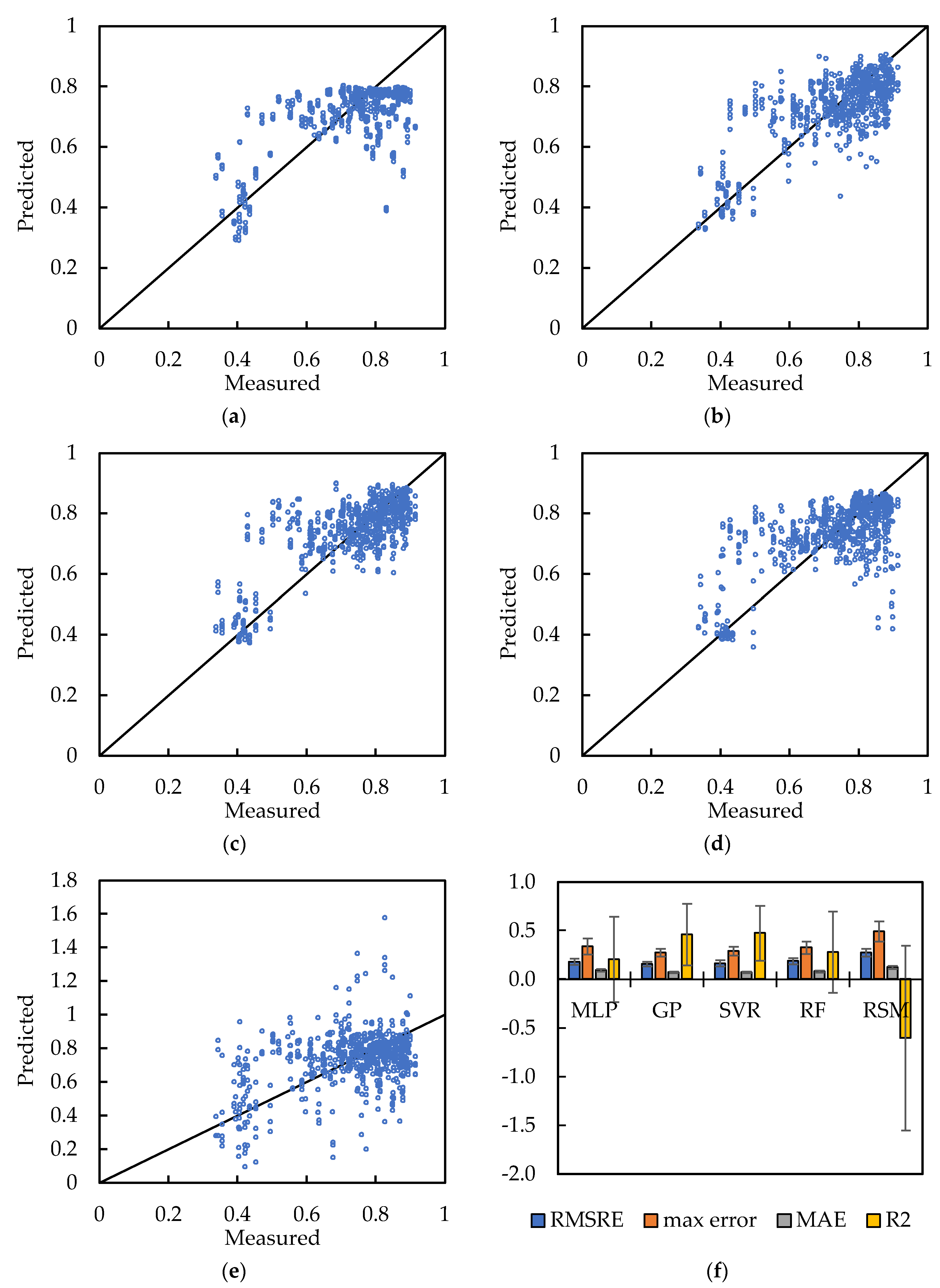
| MLP | GP | SVR | RF | RSM | |
|---|---|---|---|---|---|
| RMSRE | 0.191 | 0.145 | 0.150 | 0.203 | 0.280 |
| Max. Error | 0.440 | 0.296 | 0.301 | 0.324 | 0.619 |
| MAE | 0.091 | 0.058 | 0.062 | 0.068 | 0.125 |
| R2 | 0.206 | 0.687 | 0.650 | 0.481 | −0.630 |
| MLP | GP | SVR | RF | RSM | ||
|---|---|---|---|---|---|---|
| RMSRE | Mean | 0.180 | 0.156 | 0.164 | 0.187 | 0.274 |
| Std. Dev. | 0.031 | 0.022 | 0.033 | 0.030 | 0.038 | |
| Max. Error | Mean | 0.336 | 0.273 | 0.288 | 0.324 | 0.494 |
| Std. Dev. | 0.083 | 0.039 | 0.045 | 0.062 | 0.103 | |
| MAE | Mean | 0.091 | 0.072 | 0.071 | 0.080 | 0.123 |
| Std. Dev. | 0.014 | 0.008 | 0.008 | 0.012 | 0.017 | |
| R2 | Mean | 0.202 | 0.460 | 0.474 | 0.278 | −0.604 |
| Std. Dev. | 0.439 | 0.316 | 0.280 | 0.418 | 0.950 |
Publisher’s Note: MDPI stays neutral with regard to jurisdictional claims in published maps and institutional affiliations. |
© 2022 by the authors. Licensee MDPI, Basel, Switzerland. This article is an open access article distributed under the terms and conditions of the Creative Commons Attribution (CC BY) license (https://creativecommons.org/licenses/by/4.0/).
Share and Cite
Marques, A.E.; Dib, M.A.; Khalfallah, A.; Soares, M.S.; Oliveira, M.C.; Fernandes, J.V.; Ribeiro, B.M.; Prates, P.A. Machine Learning for Predicting Fracture Strain in Sheet Metal Forming. Metals 2022, 12, 1799. https://doi.org/10.3390/met12111799
Marques AE, Dib MA, Khalfallah A, Soares MS, Oliveira MC, Fernandes JV, Ribeiro BM, Prates PA. Machine Learning for Predicting Fracture Strain in Sheet Metal Forming. Metals. 2022; 12(11):1799. https://doi.org/10.3390/met12111799
Chicago/Turabian StyleMarques, Armando E., Mario A. Dib, Ali Khalfallah, Martinho S. Soares, Marta C. Oliveira, José V. Fernandes, Bernardete M. Ribeiro, and Pedro A. Prates. 2022. "Machine Learning for Predicting Fracture Strain in Sheet Metal Forming" Metals 12, no. 11: 1799. https://doi.org/10.3390/met12111799
APA StyleMarques, A. E., Dib, M. A., Khalfallah, A., Soares, M. S., Oliveira, M. C., Fernandes, J. V., Ribeiro, B. M., & Prates, P. A. (2022). Machine Learning for Predicting Fracture Strain in Sheet Metal Forming. Metals, 12(11), 1799. https://doi.org/10.3390/met12111799