Stress Rupture Life Prediction Method for Notched Specimens Based on Minimum Average Von Mises Equivalent Stress

Abstract

Creep tests were carried out on notched plate specimens of nickel-based superalloy GH4169 with different stress concentration coefficients. It was found that the duration of the first stage of the creep curve increases with the increase of stress concentration coefficient, while the fracture ductility decreases with the increase of stress concentration coefficient. To predict the life of notched plate specimens, four constitutive models were used to analyze the stress and strain of the notches. It was found that the average Von Mises equivalent stress (AVES) on the minimum notch section first decreases and then increases with the creep time, resulting in a minimum value. The minimum average Von Mises equivalent stress (MAVES) is considered as the characteristic stress of notched specimens in this paper. The creep life equation is fitted according to the results of creep tests of smooth specimens, and then the predicted life of notched specimens is obtained by substituting the minimum average Von Mises equivalent stress of notched specimens into the creep equation. The prediction results of the four constitutive models are within 2 times the dispersion band, and the three-stage model is within the 1.5 times dispersion band.

1. Introduction

The hot section components of aero-engine often operate at relatively high temperatures for a prolonged time. The complex loads and irregular shapes result in a multiaxial state of stress in the components. To study the creep behavior of this kind of component in the complex working environment and predict their life, the first step is to accurately predict the stress rupture life of notched specimens under a laboratory environment.

The research on the rupture life of notched specimens at high temperatures has gradually increased since the 1970s, among which the notched round bar specimens are widely researched. The commonly used methods include the skeletal point method [1,2,3,4,5,6], the multi-axial ductility exhaustion method [7,8,9,10,11], and the prediction method based on AVES [12]. These methods cannot be operated without the finite element analysis of notched specimens. Hayhurst [6] et al. used skeletal point stress for the prediction of rupture life. They found that in the process of stress redistribution, there was a point at the minimum cross-section where the stresses are nearly constant. The skeletal point stresses have been used to characterize the deformation and failure behavior of the material under multiaxial creep conditions. This model is suitable for notched round bar specimens to find the skeletal point along the radius direction. While if the cross-section of the specimen is rectangular or irregular like that in the real components, it is not easy to find the skeletal point. The multi-axial ductility exhaustion approach establishes the relationship between uniaxial and multiaxial creep ductility through the multiaxial ductility factor, which is generally a function of hydrostatic pressure. Webster and Pickard [12] performed finite element analysis on the notched specimens and obtained the AVESes at a certain time. Using the concept of critical rupture ductility (i.e., creep failure through ductility exhaustion), strain accumulation is assumed to follow the steady-state rate consistent with the AVES until the rupture ductility is reached.

It is necessary to carry out a large number of long-term creep experiments to obtain the creep ductility curve. This paper proposes a new method for predicting rupture life based on AVESes, without using the concept of critical rupture ductility. According to our research, it is found that the AVES at the minimum cross-section of notched specimens first decreases and then increases with time, so there exists a MAVES. The MAVES is taken as the characteristic stress and is substituted into the creep life equation to obtain the rupture life of notched specimens. The influence of four different creep constitutive equations and three different creep life equations on the life prediction is analyzed in this paper.

2. Experiment and Results

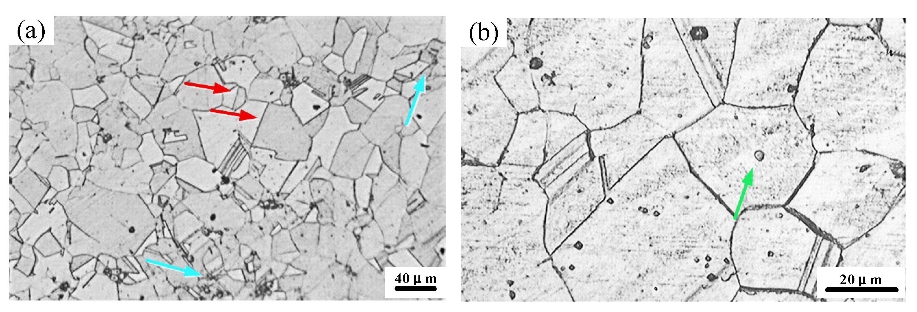
2.1. Composition and Microstructure Characterization

GH4169 is a precipitation strengthening nickel-based superalloy with good fatigue and corrosion resistance. It is widely used in aero-engine rotor components, such as high-pressure compressor disks and turbine disks. The composition of GH4169 is similar to that of the nickel-based superalloy IN718 [13], as shown in

Table 1. Composition of Ni-based superalloy GH4169.

Element	Cr	Ti	Fe	Mo	Al	Nb
Wt%	17.00~21.00	0.75~1.15	14.2~24.0	2.80~3.30	0.30~0.70	5.00~5.50
Element	N	C	Mn	Si	P	Ni
Wt%	≤0.01	0.015~0.006	≤0.35	≤0.35	≤0.015	Bal.

.

A small piece of material is taken from the original material for metallographic testing. The metallographic specimen was subjected to 6 rounds of rough polishing and 1 round of final polishing. The order of coarsely polished sandpaper was 800#, 1000#, 1500#, 2000#, 3000# to 5000#, and the final polishing process was performed using NonDry suspension and polishing cloth for 3–5 min. Finally, the specimen is immersed in the corrosion solution for 1–5 s. The composition of the corrosion solution is 80 mL hydrochloric acid +40 mL methanol +40 g copper chloride.

The metallographic structure of the virgin material of GH4169 alloy is shown in Figure 1. In low magnification microscope photos (Figure 1a), the twin structure is marked by the red arrows, and the local area of grain refinement is marked by blue arrows. It can be observed that the grain size distribution of the material is not very uniform. Large grains have diameters of more than 50 μm, while fine grains have diameters of 10–20 μm, and fine grains are mainly concentrated in local areas. At high magnification, inclusions in the material can be seen, the size of which is 1–10 μm, mainly distributed in the grain interior.

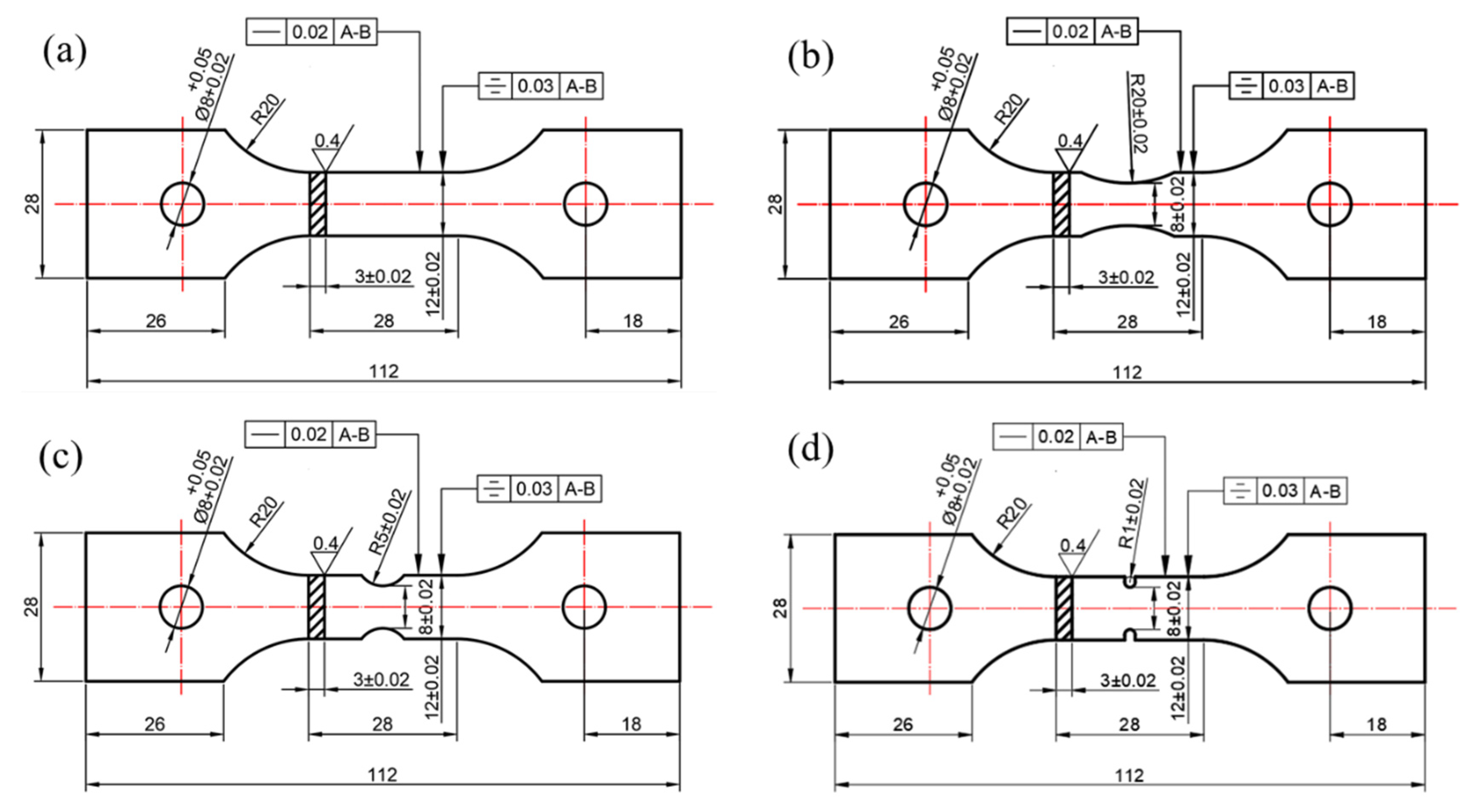
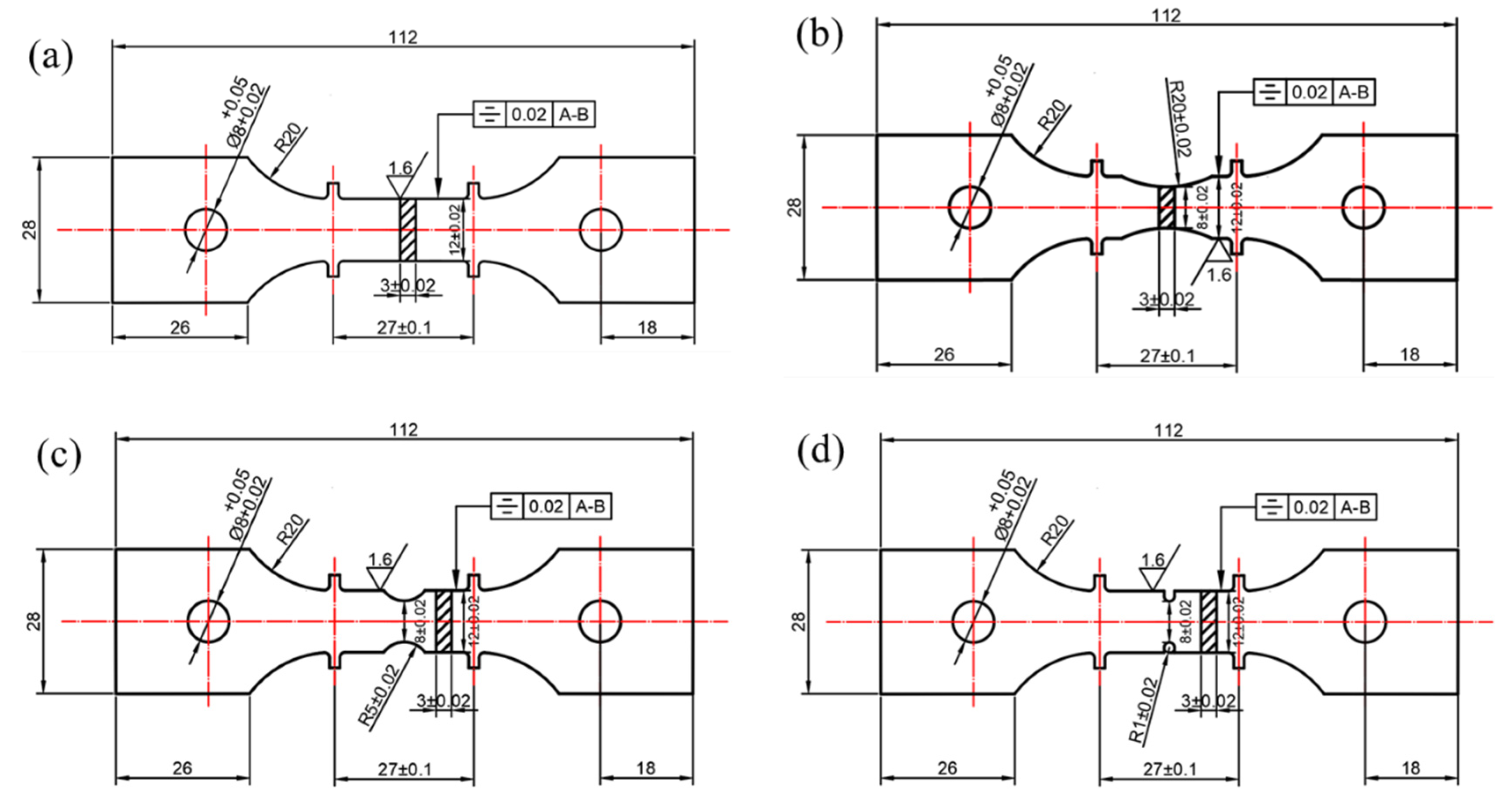
2.2. Specimens and Test

In this paper, three kinds of notched and a kind of unnotched plate specimens were designed. Notches in all notched specimens are of the same depth but with different radii, R = 1 mm, 5 mm, and 20 mm, respectively. The detailed dimensions of tensile and creep specimens are shown in Figure 2 and Figure 3. The only difference between the tensile and creep specimens is the presence or absence of convex plates. The strain of the tensile specimen was measured using a laser-type non-contact extensor, so tensile specimens have no convex plates. The strain of the creep specimen was measured with a clamp-type extensometer, which needed to be clamped on the convex plates at both ends.

Tensile and creep tests were carried out in air at 650 °C. Prior to applying load, all specimens were incubated at the test temperature for 30–60 min to ensure the uniform temperature inside the specimens. Each kind of creep specimen was tested for 5–6 loads, one for each load.

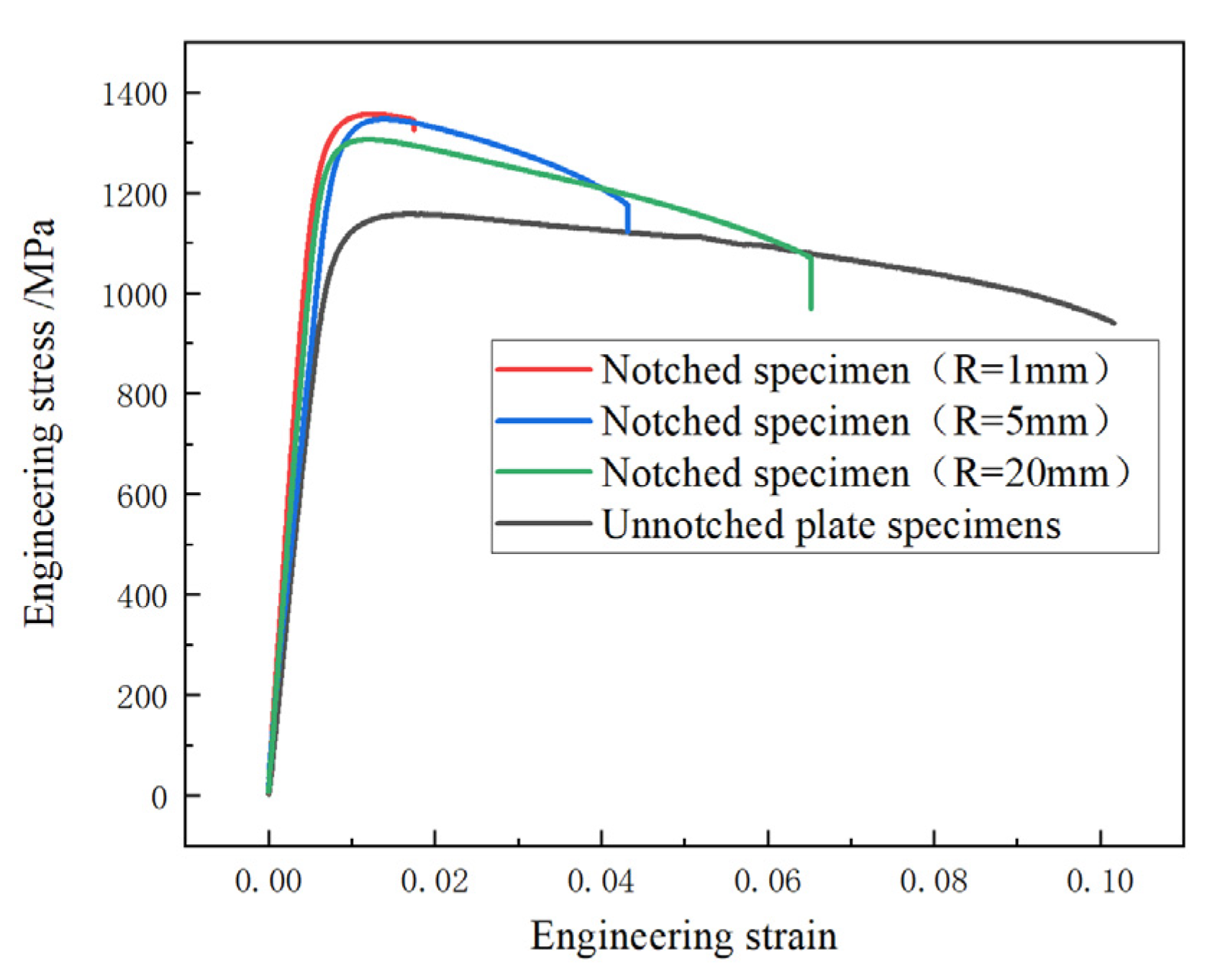
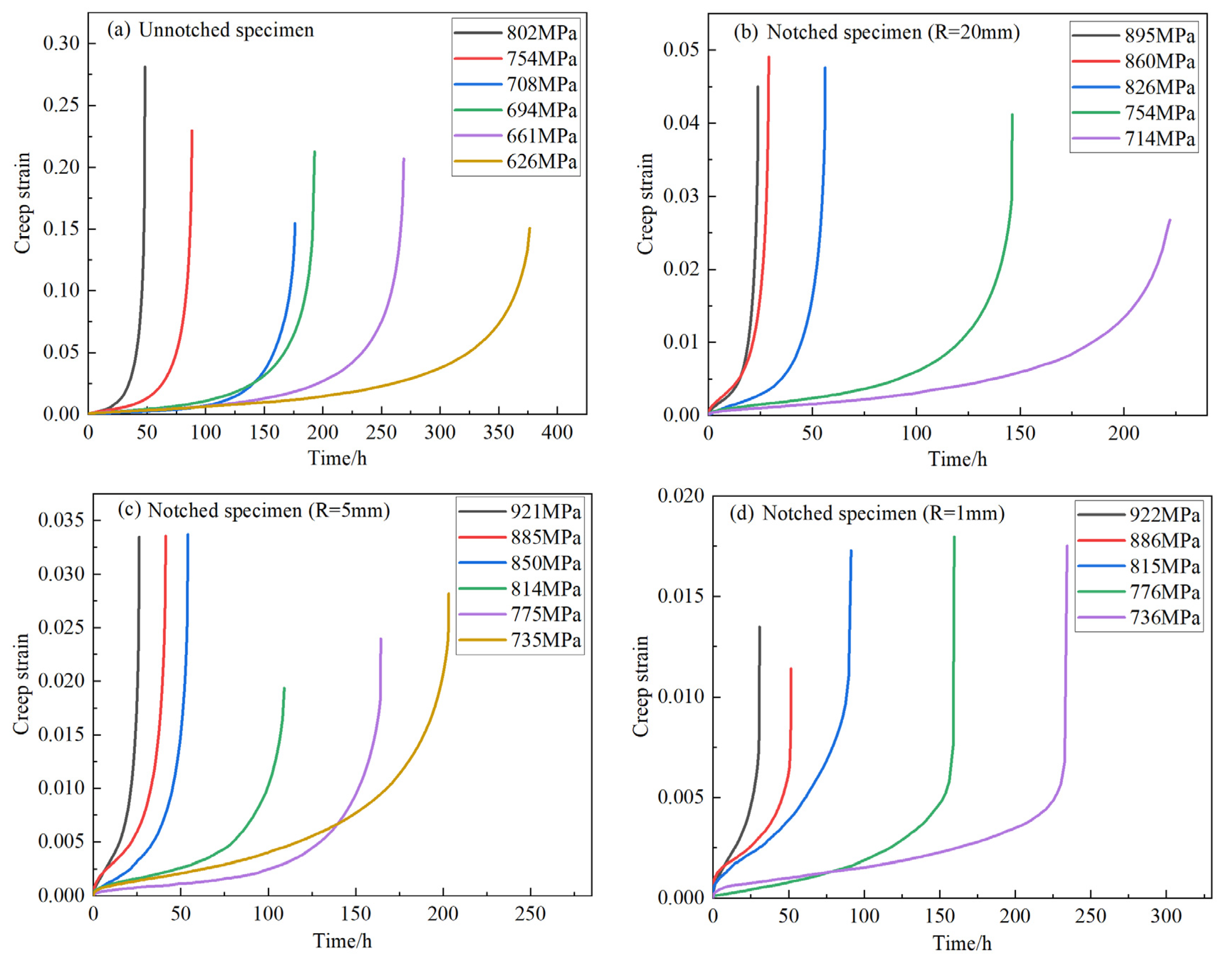
2.3. Experimental Results

The tensile nominal stress vs. strain curves of unnotched and notched specimens are shown in Figure 4. The elastic modulus and ultimate strength of the notched plate are both higher than those of the unnotched plate, and the rupture strain is smaller than that of the unnotched plate. For notched specimens, the ultimate tensile strength increases, and the fracture strain decreases when the notch becomes sharper.

The first stage of creep of the unnotched creep test curve is not obvious, as shown in Figure 5a. But with the increase of notch stress concentration, the first stage of creep becomes more and more obvious, as shown in Figure 5b–d.

3. Life Prediction Method

3.1. Constitutive Model

The creep analysis of notched specimens is inseparable from the finite element analysis. To understand the internal stress and strain distribution of notched specimens more clearly, it is necessary to establish the elastic-plastic coupled creep model based on tensile and creep experiments results of the material, and establish the finite element model of notched specimens by applying fixed constraints on one end of the specimens and concentrated forces on the other end.

The constitutive equation consists of the elastic-plastic constitutive coupled with creep constitutive, and the calculation process is divided into two steps: the first step is elastic-plastic loading, and the second step is creep loading. The multilinear isotropic hardening model is selected as the elastic-plastic constitutive model, and four creep constitutive models are used for comparative analysis. Since the first stage of creep experiment results (as shown in Figure 5) is not obvious, two creep constitutive models which only describe the second stage of creep are selected in this paper, and the other two creep constitutions can describe the three stages of the creep curve.

Because the notched specimen has a certain stress concentration at the minimum cross-section, the locations where the stress is concentrated will enter plasticity earlier than other locations, and the deformation of the specimen will mainly concentrate at the notch. Considering the large deformation caused by the notched position, the elastoplastic parameters of the material need to be fitted by true stress-true strain, and the conversion formulas are as follows:

σ = σ_e (1 + ε_e)

(1)

ε = ln (1 + ε_e)

(2)

where σ is true stress, ε is true strain, σ_e is engineering stress, and ε_e is engineering strain.

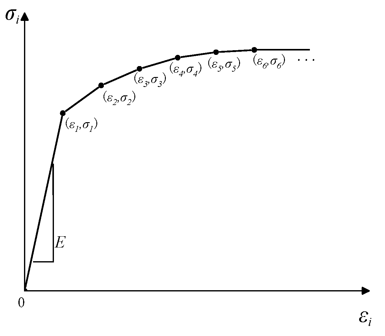
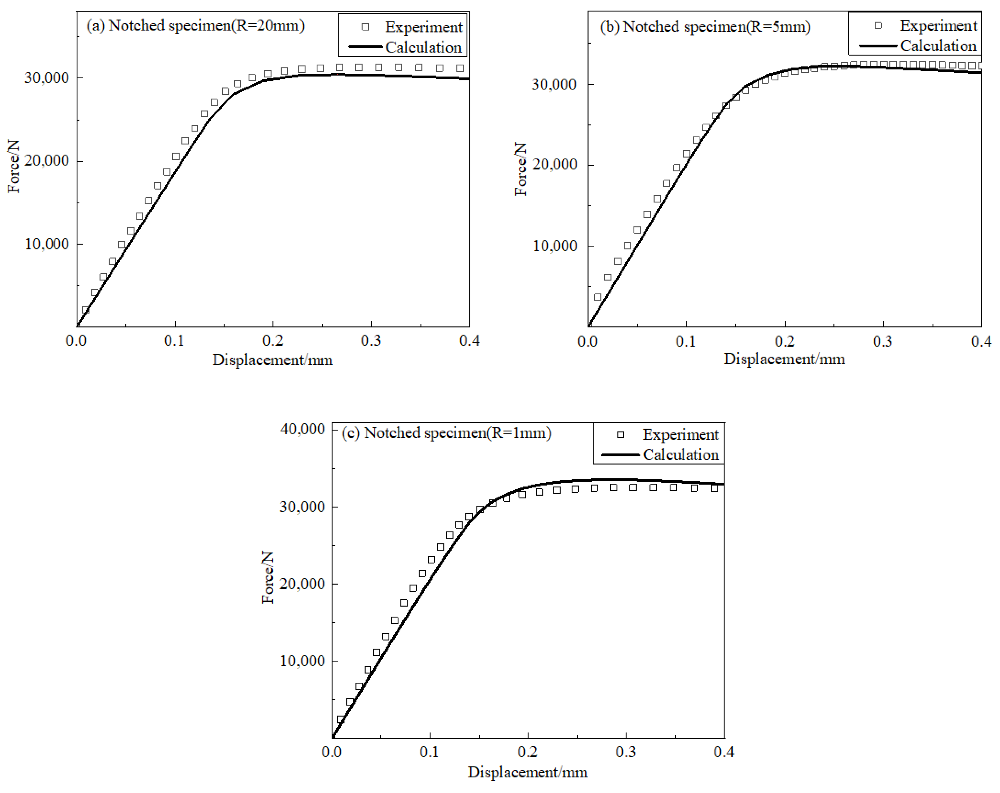
3.1.1. Multilinear Isotropic Hardening Constitutive Model

The multilinear isotropic hardening behavior is described by a piece-wise linear stress-total strain curve, starting at the origin and defined by sets of positive stress and strain values, as shown in Figure 6. The first point (ε₁, σ₁) in the model is the yield point. Theoretically, the more points selected in the curve, the more accurate the model will be. However, there can be no infinite points. In this paper, 20 points are used.

The elastic-plastic parameters obtained by fitting the tensile data of the unnotched specimens were input into the ANSYS for simulating the tensile properties of notched specimens. The relationship between the displacement of the gauge segment and the loading force was obtained by the finite element calculation. The results are shown in Figure 7. The experimental and calculated values of maximum loading are very close, with errors of −1.6% (R = 20 mm), 0% (R = 5 mm), and −2.2% (R = 1 mm), respectively. The tensile behavior of notched specimens can be well described by the multilinear isotropic hardening constitutive.

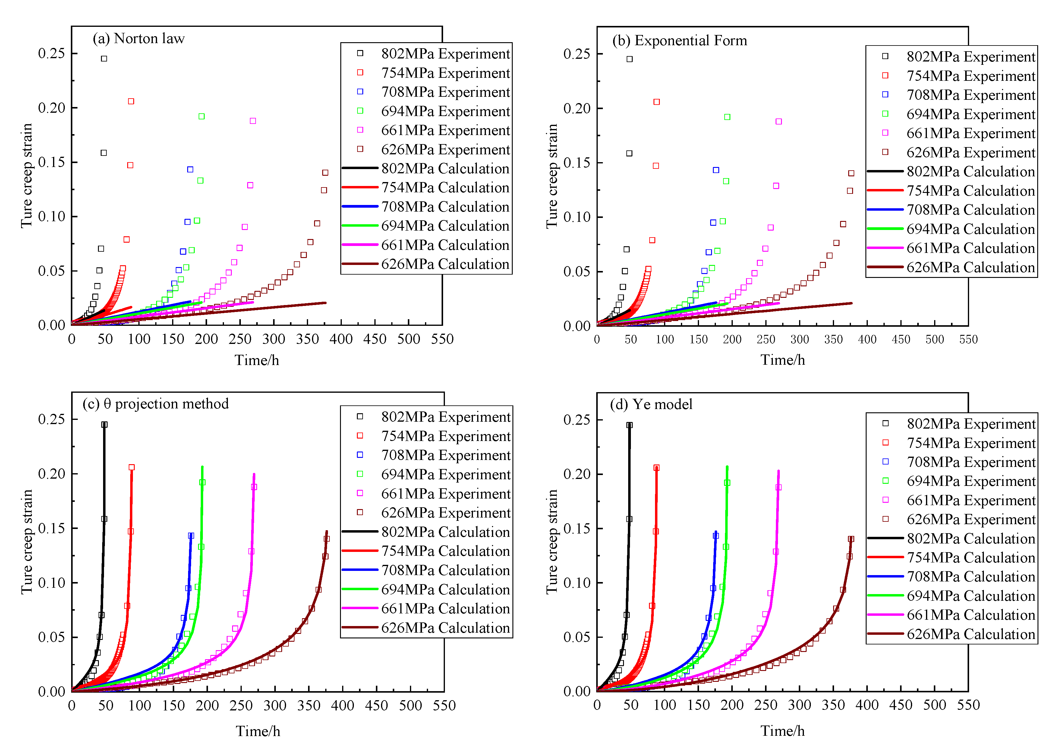
3.1.2. Creep Constitutive Model

Two creep constitutive models which only describe the second stage and two creep constitutive models capable of describing the three stages of creep were selected. The creep constitutive models capable of describing the whole process of creep were embedded into the finite element software ANSYS interface program usercreep f.

1.

Norton law

$${\dot{\epsilon }}^c=A{\sigma }^n$$

(3)

where A and n are material constants.

2.

Exponential form

$${\dot{\epsilon }}_c=B\exp (\sigma /d)$$

(4)

where B and d are material constants.

3.

θ Projection approach

The principle of the θ Projection approach is that creep curves under uniaxial constant stress measured over a range of stresses and temperatures can be “projected” to other stress/temperature conditions and then reconstruct the complete creep curves [14]. The θ Projection approach can be written as the sum of two terms, as shown in equation (5). It is considered that the creep curve is the sum of the first stage of attenuation and the third stage of acceleration, and the second stage of relative stability is a process of the relative balance between attenuation and acceleration [15].

$${\epsilon }^c={\theta }_1(1-e^{-{\theta }_{2}t})+{\theta }_3(e^{{\theta }_{4}t}-1)$$

(5)

where θ₁ and θ₃ are “scaling” parameters that define the extent of the primary and tertiary creep with respect to strain. Whereas θ₂ and θ₄ are “rate” parameters characterizing the curvature of the primary and tertiary creep curves [16,17]. The effect of temperature is not considered in this paper, so θ value is written as a function of stress and temperature:

$$\lg {\theta }_i=b_i+f_i\sigma$$

(6)

where b_i, f_i (i = 1, 2, 3, 4) are material parameters.

4.

Ye model

The Ye model was recently developed by our research team [18]. The creep constitutive replaces the nominal stress in the traditional creep model with the normalized stress of tensile strength and can describe the whole process of creep.

$${\dot{\epsilon }}^c=\frac{\beta }{\left(\delta t+\varsigma \right)\ln \left(\delta t+\varsigma \right)}+\mu c_6{t}^{c_6-1}$$

(7)

where

$$\beta =-{\left(\frac{\sigma }{{\sigma }_{UTS}}\right)}^{c_3}\exp \left(c_4\right)$$

(8)

$$\delta ={\left(\frac{\sigma }{{\sigma }_{UTS}}\right)}^{c_1}\exp \left(c_2\right)$$

(9)

$$\mu ={\left(\sigma /{\sigma }_{UTS}\right)}^{c_7}\exp \left(c_8\right)$$

(10)

where σ_UTS is ultimate tensile strength, c₁–c₈ are material constants.

The constitutive parameters are listed in

Table 2. Parameters of constitutive models.

Norton law	A	n
	1.62 × 10−3	6.625
Exponential form	B	d
	1.41 × 10−7	104.68
θ projection method	b1	b2	b3	b4	f1	f2	f3	f4
	−0.885	−10.2	−5.50	−2.05	−1.1 × 10−4	9.7 × 10−3	5.1 × 10−3	−2.42 × 10−4
Ye model	c1	c2	c3	c4	c5	c6	c7	c8
	1.955	6.726	−10.5	16.74	−9.26	1.0 × 10−5	19.31	−9.41

, and the fitting results are shown in Figure 8. Norton law and exponential form can describe the second stage of creep well, and the θ-projection method and Ye model almost fit perfectly.

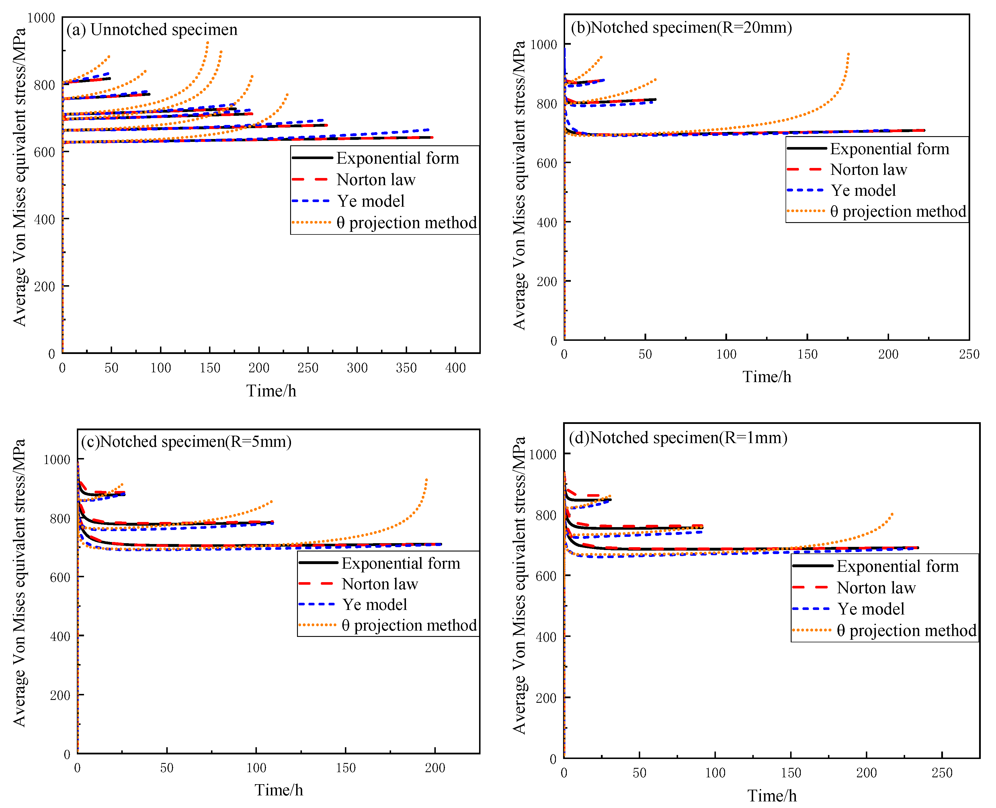
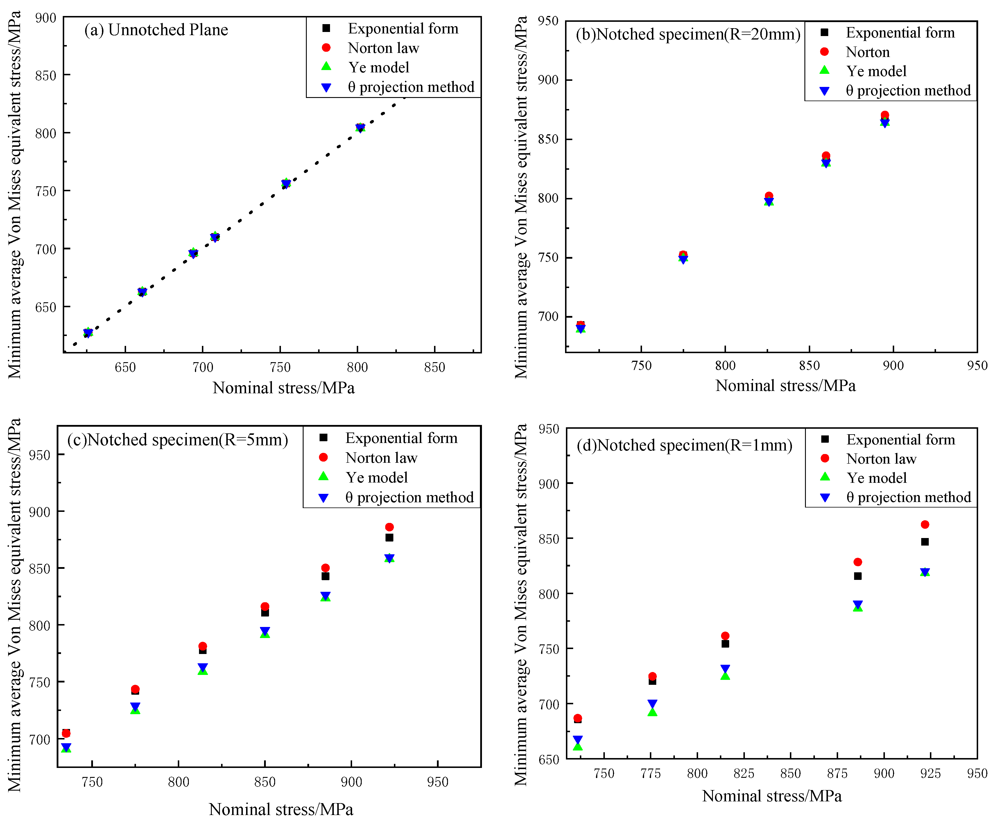
3.2. Von Mises Equivalent Stress

Since the Von Mises equivalent stress was distributed unevenly on the cross-section, the concept of AVES was introduced to characterize the Von Mises equivalent stress of the whole cross-section. The AVES is obtained by adding the equivalent stress over small increments of the area and divided by the total area as shown in Equation (11).

$${\overline{\sigma }}_{VM}=\frac{1}{A}{\int }_0^A{\sigma }_{VM}dA$$

(11)

The curves of AVES with time are shown in Figure 9. The shape of the curves are similar to whatever the constitutive model used. The AVES of unnotched specimens increased slowly during creep, while the AVES of notched specimens first decreased rapidly and then increased slowly with time. The shape of the curves is similar to the stress-relaxation curves of the material. This is because in the initial stage of creep, the total displacement of the notched specimen varied extraordinarily little, and the stress on the notched section was higher than that on other sections. So, the stress on the notched section was redistributed. During the creep process of the notched specimen, the minimum notched cross-section began to shrink, resulting in the moderate increase of the AVES. If the small deformation finite element calculation was used rather than the large deformation calculation, the AVES of the smallest section would not increase after reaching the minimum value.

The relationship between the minimum value of AVES and the nominal stress of different notches and constitutive models is shown in Figure 10. The MAVES of the unnotched specimen is the same as the nominal stress loaded. With the increase of notch stress concentration coefficient, the difference of the MAVES calculated by different constitutive models gradually increases. The MAVES calculated by the second stage model is larger than that calculated by the whole stage model. The calculation results of the same type of creep constitutive models are very close.

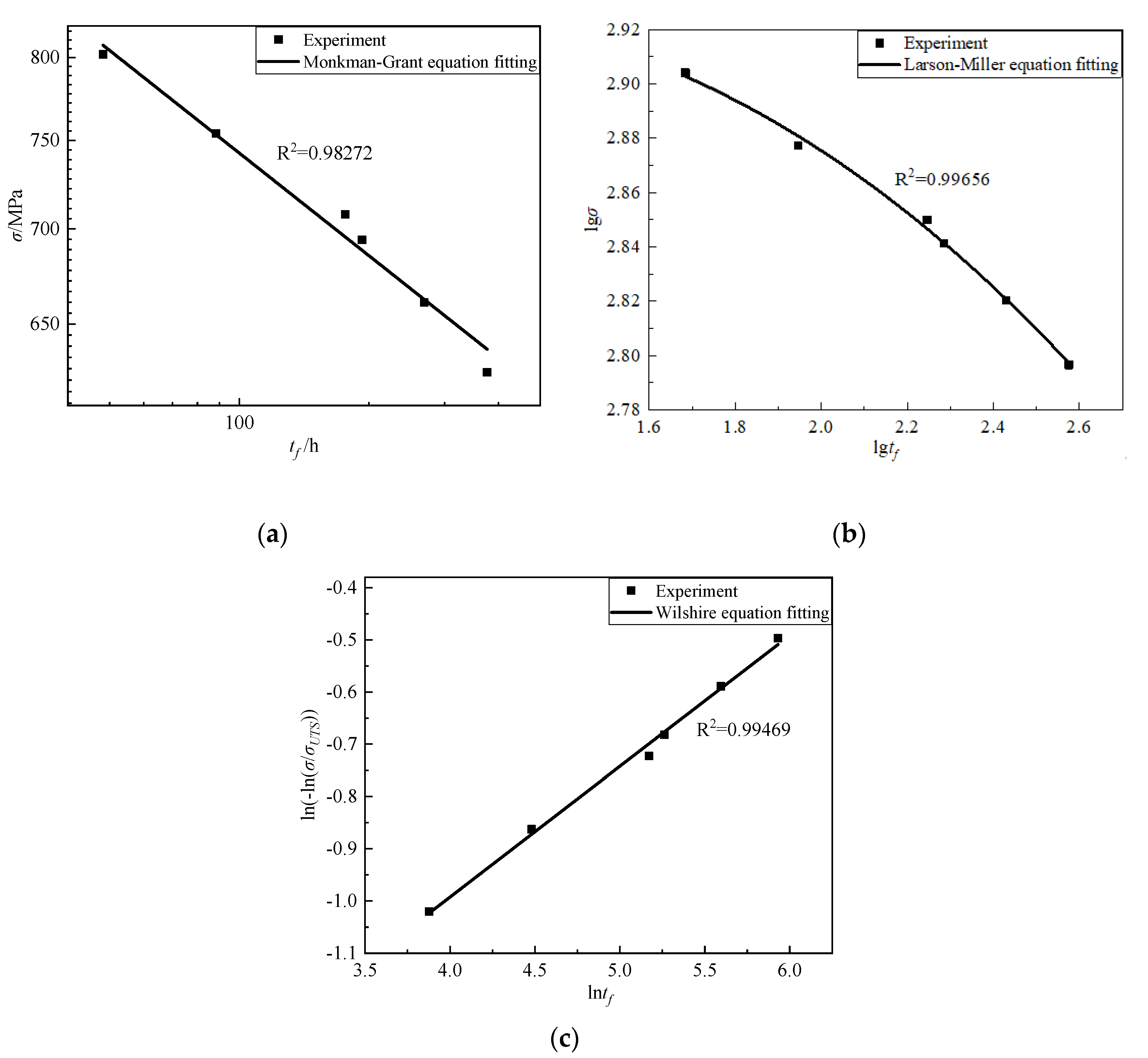
3.3. Creep Life Equation

Three creep life equations are applied to evaluate notched specimen life prediction based on the MAVES. The Monkman–Grant equation [19,20,21,22] and the Larson–Miller equation [22,23,24,25,26], developed in the 1950s, are still widely used today. The latest creep life equation, developed by Wilshire et al. [27], has been rapidly applied to the study of creep properties of different materials [28,29,30,31,32].

• Monkman–Grant equation

Monkman and Grant [19] found a functional relationship between creep rupture life and the minimum creep rate of materials. They proposed a power law equation, containing the Arrhenius term, where the minimum creep rate is related to the creep life through the Monkman–Grant relationship as shown in Equation (12):

$$M/t_f={\dot{\epsilon }}_m^c=A^{\prime }{\sigma }^{n^{*}}\exp (-Q_c/RT)$$

(12)

where M is the Monkman–Grant constant, A’ and n* are material parameters, Q_c are the parameters related to the activation energy, R is the gas constant, and T is the absolute temperature. As there is only one loading temperature in this paper, the equation can be simplified as:

$$t_f=A^{″}{\sigma }^{n^{*}}$$

(13)

2.

Larson–Miller equation

The Larson–Miller equation expresses the life t_f and temperature T as the endurance thermal strength parameter P. Thus, the empirical relationship between the stress and the durable thermal strength parameters is established as follows:

$$\begin{gathered} P=T(C_{LM}+\log t_f) \\ \log (\sigma )=a_1+a_{2}P+a_3{P}^2+a_4{P}^3 \end{gathered}$$

(14)

where C_LM is the Larson–Miller constant and P is the parameter related to temperature and life.

3.

Wilshire equation

In recent years, a research group at the University of Swansea has proposed a creep data processing method (called the Wilshire equation) based on the microscopic deformation mechanism of materials.

$$\left(\sigma /{\sigma }_{UTS}\right)=\exp \left\{-k_1{\left[t_f\exp \left(-Q_c^{*}/RT\right)\right]}^u\right\}$$

(15)

where σ_UTS is the ultimate tensile strength of the material, and Q_c* is the parameter related to the activation energy. k₁ and the exponent u are material constants. Q_c* is fitted by the creep test results at different temperatures. The experiments were carried out only at 650 °C, therefore, the equation can be simplified as

$$(\sigma /{\sigma }_{UTS})=\exp (-k_1^{\prime }{t}_f{}^{\mu })$$

(16)

The fitting parameters of the three creep life equations are shown in

Table 3. Parameter values of the life equation.

Monkman–Grant equation	A″	n*
	1263	−0.1153
Larson–Miller equation	a1	a2	a3	a4	CLM	T
	2.585	11.80	137.82	−5545	3.023	923.15
Wilshire equation	σUTS	k1′	u
	1150	0.1336	0.254

. The fitting results are shown in Figure 11. Regardless of the creep life equation selected, there is a certain error at 708 MPa. This may be due to experimental error. The fitting degree of the regression curve to the observed value is called goodness of fit. The metric statistic of the goodness of fit is the determination coefficient, which is represented by the symbol R². The maximum value of R² is 1, and the closer R² is to 1, the better the fitting degree of the regression curve to the observed value is. Instead, the smaller the value of R², the worse the fitting degree of the regression curve to the observed value is. Consequently, it can be observed that the results fitted by the Monkman–Grant equation are worst among the three models, and the results fitted by Larson–Miller equation and Wilshire equation are similar.

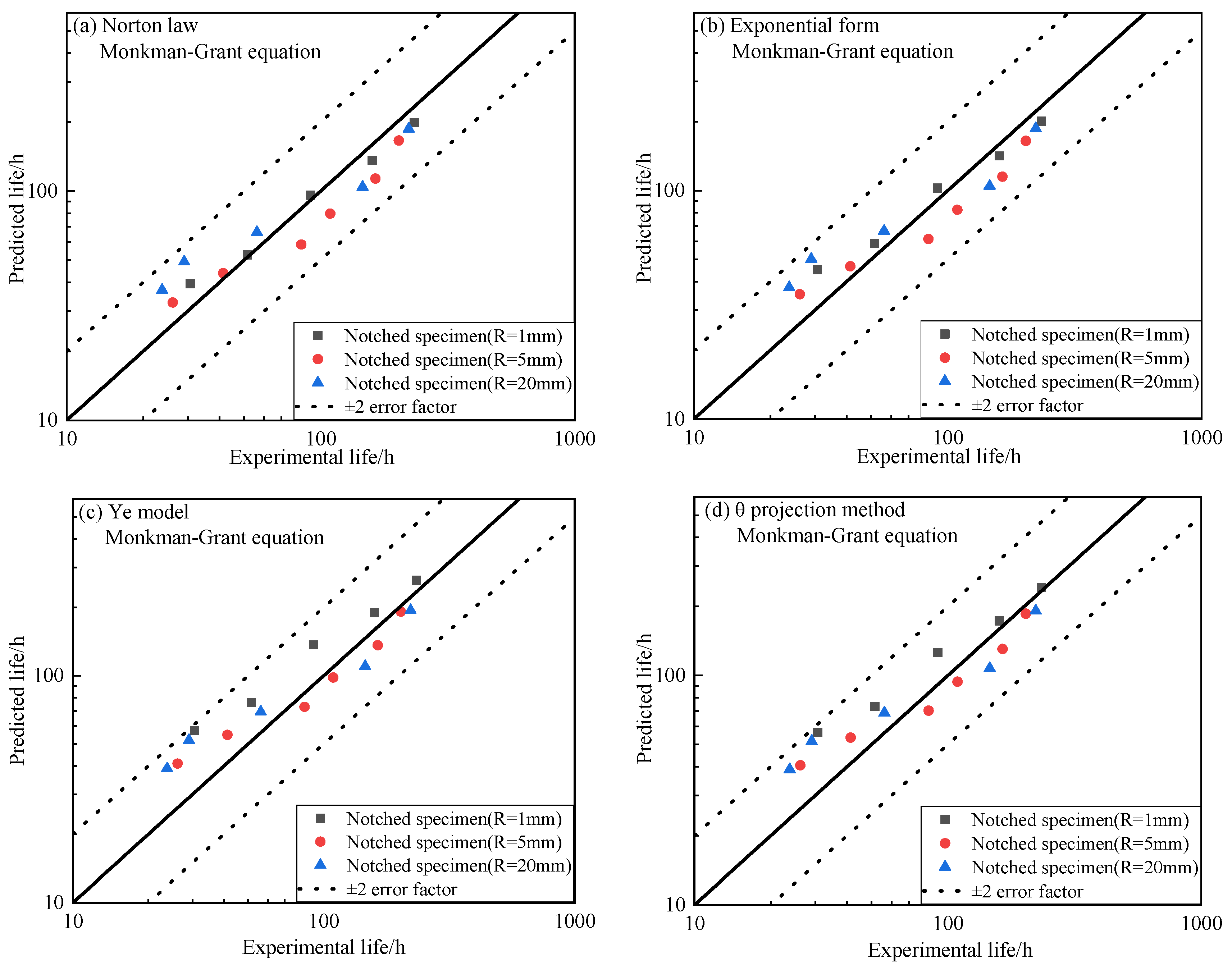
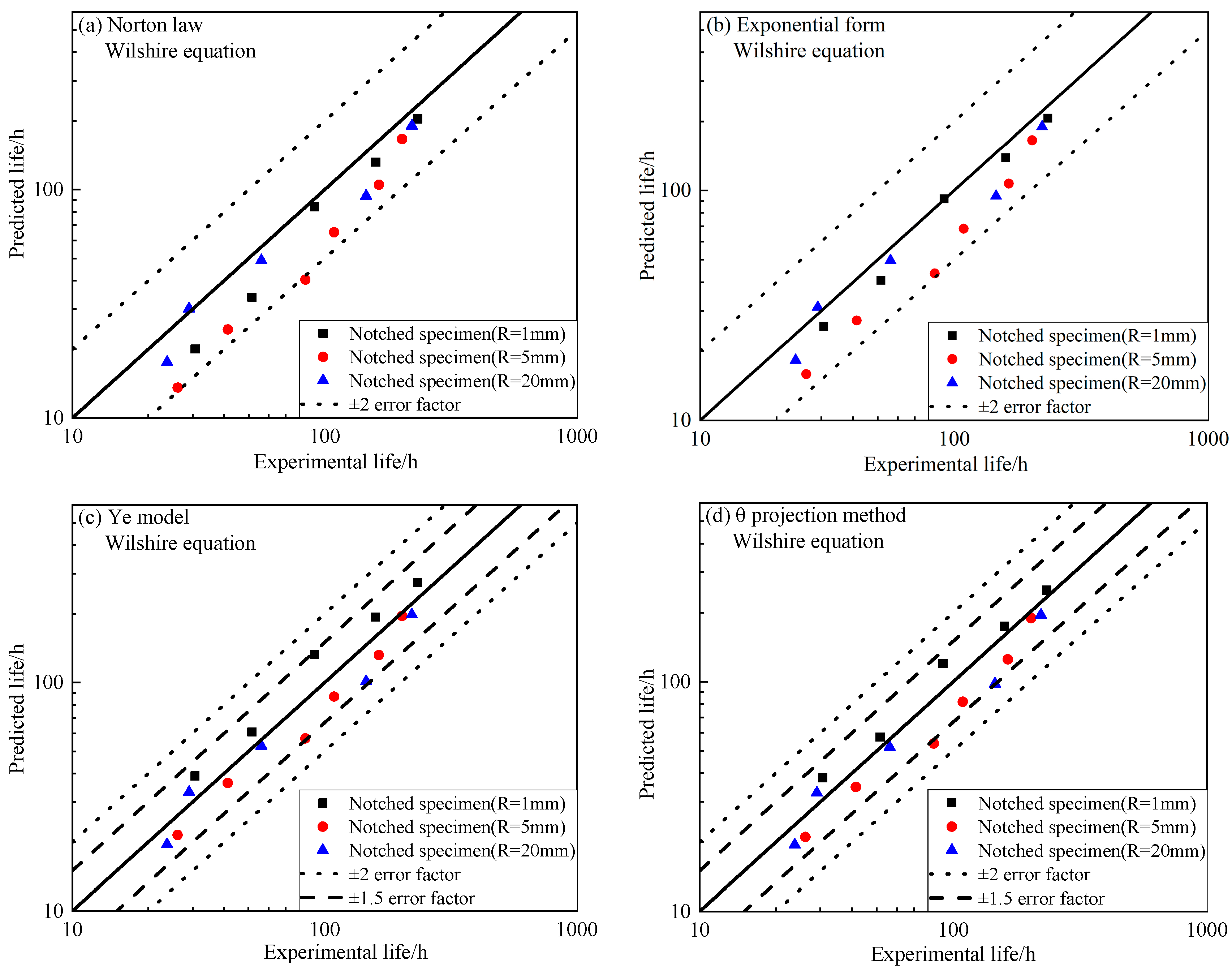
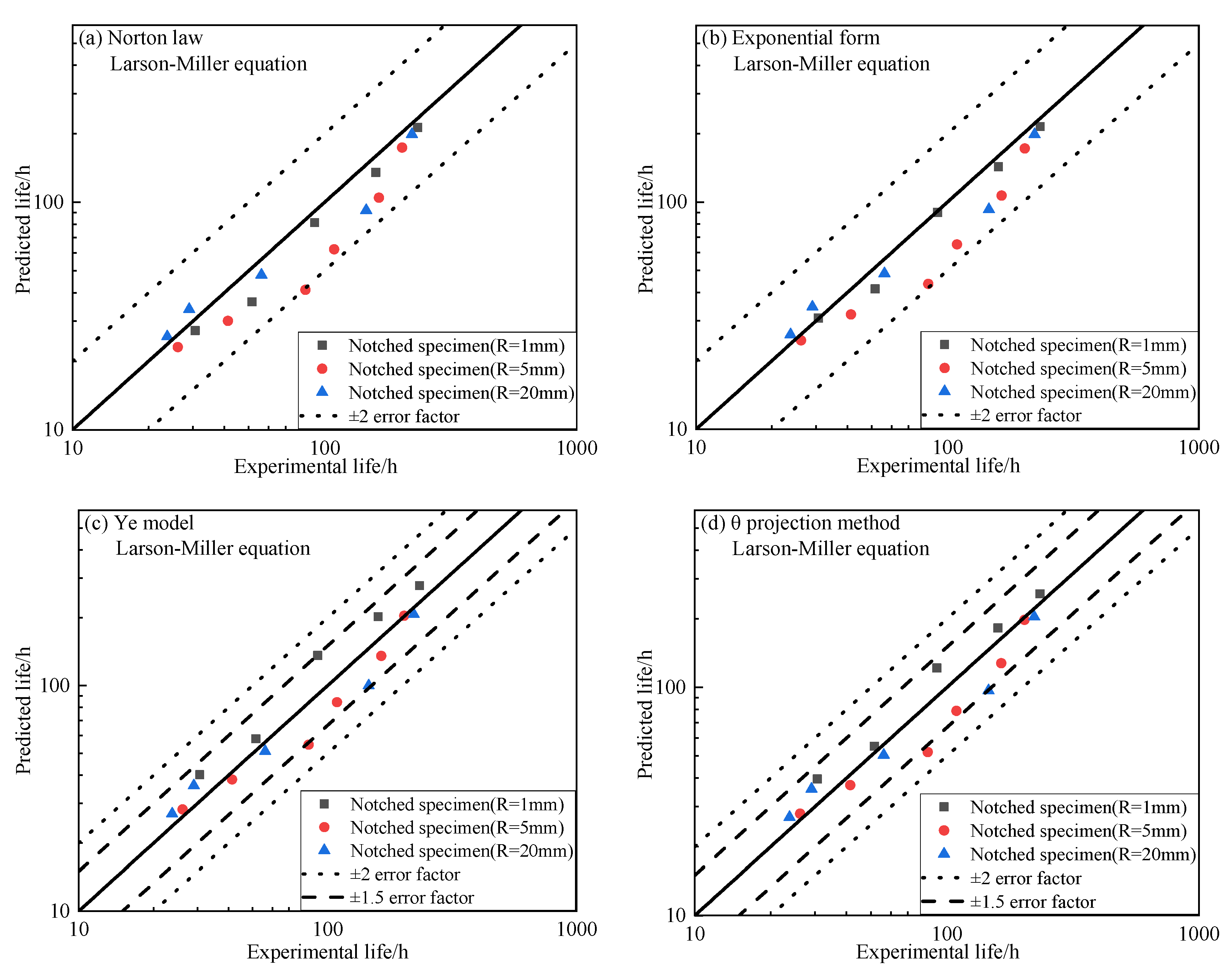
3.4. Analysis of Prediction Results

The MAVES calculated by all constitutive models were substituted into different life prediction equations, and the results are shown in Figure 12, Figure 13 and Figure 14. Whichever constitutive model and life prediction method are selected, the stress rupture life prediction results of the notched specimens are almost within the double dispersion band. Because the difference of the MAVES of the same constitutive type is very small, the life prediction results of notched specimens are close.

If the creep constitutive model capable of describing the whole process of creep and the life equation of the Wilshire equation or Larson–Miller equation are used, the prediction result will be the most ideal, which are almost within the 1.5 times dispersion band. The higher accuracy of prediction results maybe because the calculation results of the three-stage model are closer to the real load conditions.

No matter which constitutive model is selected, the results predicted by Monkman–Grant equation are all in the double dispersion band. The extrapolation ability of Monkman–Grant equation is insufficient, leading to the characteristic of small predicted values for the short-lived case as shown in Figure 13. Monkman–Grant equation has its limitations, especially in long-term data prediction based only on short-term experiments results [30], which is why the short-life prediction results in this paper are too large, as shown in Figure 13.

The prediction results are always smaller than the test results when the second-stage creep constitutive model and the Wilshire equation are selected. This life prediction method is conservative and commercial. The software usually has its own second-stage creep constitutive model. Therefore, the combination of the second-stage constitutive model and the Wilshire equation has good prospects in engineering application.

4. Conclusions

Based on the creep experiments on unnotched and notched specimens and finite element analysis with different constitutive models, the following conclusions have been drawn.

• The change rule of AVES with time is that it first decreases rapidly and then increases slowly, so there is a minimum value of AVES.
• With the increase of notch stress concentration coefficient, the MAVES calculated by the second stage model is larger than that calculated by the whole stage model.
• Whatever the life equation or constitutive model is used, the results of notch life prediction using MAVES as the characteristic stress are within 2 times the dispersion band. If a three-stage creep constitutive model is used, the predicted results are scattered within a factor of 1.5.

References

1. Al-Faddagh, K.D.; Fenner, R.T.; Webster, G.A. Steady-state stress distributions in circumferentially notched bars subjected to creep. J. Strain Anal. Eng. Des. 1982, 17, 123–132. [Google Scholar] [CrossRef]
2. Hayhurst, D.R.; Webster, G.A. An overview on studies of stress state effects during creep of circumferentially notched bars. In Techniques for Multiaxial Creep Testing; Springer: Berlin/Heidelberg, Germany, 1986; pp. 137–175. [Google Scholar]
3. Hyde, T.H.; Xia, L.; Becker, A.A. Prediction of creep failure in aeroengine materials under multi-axial stress states. Int. J. Mech. Sci. 1996, 38, 385–403. [Google Scholar] [CrossRef]
4. Eggeler, G.; Wiesner, C. A numerical study of parameters controlling stress redistribution in circular notched specimens during creep. J. Strain Anal. Eng. Des. 1993, 28, 13–22. [Google Scholar] [CrossRef]
5. Webster, G.A.; Nikbin, K.M.; Biglari, F. Finite element analysis of notched bar skeletal point stresses and dimension changes due to creep. Fatigue Fract. Eng. Mater. Struct. 2004, 27, 297–303. [Google Scholar] [CrossRef] [Green Version]
6. Hayhurst, D.R.; Henderson, J.T. Creep stress redistribution in notched bars. Int. J. Mech. Sci. 1977, 19, 133–146. [Google Scholar] [CrossRef]
7. McClintock, F.A. A Criterion for Ductile Fracture by the Growth of Holes. J. Appl. Mech. 1968, 35, 363–371. [Google Scholar] [CrossRef]
8. Cocks, A.; Ashby, M.F. Intergranular fracture during power-law creep under multiaxial stresses. Met. Sci. 1980, 14, 395–402. [Google Scholar] [CrossRef]
9. Wen, J.F.; Tu, S.T. A multiaxial creep-damage model for creep crack growth considering cavity growth and microcrack interaction. Eng. Fract. Mech. 2014, 123, 197–210. [Google Scholar] [CrossRef]
10. Spindler, M.W. The multiaxial and uniaxial creep ductility of Type 304 steel as a function of stress and strain rate. High Temp. Technol. 2004, 21, 47–54. [Google Scholar] [CrossRef]
11. Wen, J.F.; Tu, S.T.; Xuan, F.Z.; Zhang, X.W.; Gao, X.L. Effects of stress level and stress state on creep ductility: Evaluation of different models. J. Mater. Sci. Technol. 2016, 32, 695–704. [Google Scholar] [CrossRef]
12. Webster, P.S.; Pickard, A.C. The prediction of stress rupture life of notched specimens in the beta-processed titanium alloy Ti5331s. J. Strain Anal. Eng. Des. 1987, 22, 145–153. [Google Scholar] [CrossRef]
13. Wang, R.-Z. Creep-fatigue behaviors and life assessments in two nickel-based superalloys. J. Press. Vessel. Technol. 2018, 140, 031405. [Google Scholar] [CrossRef]
14. Abdallah, Z.; Gray, V.; Whittaker, M. A critical analysis of the conventionally employed creep lifing methods. Materials 2014, 7, 3371–3398. [Google Scholar] [CrossRef] [PubMed] [Green Version]
15. Kim, W.G.; Yin, S.N.; Kim, Y.W.; Chang, J.H. Creep characterization of a Ni-based Hastelloy-X alloy by using theta projection method. Eng. Fract. Mech. 2008, 75, 4985–4995. [Google Scholar] [CrossRef]
16. Evans, R.W.; Scharning, P.J. The θ projection method applied to small strain creep of commercial aluminum alloy. Mater. Sci. Technol. 2001, 17, 487–493. [Google Scholar] [CrossRef]
17. Evans, R.W.; Wilshire, B. The role of grain-boundary cavities during tertiary creep. In Creep and Fracture of Engineering Materials and Structures; Wilshire, B., Owen, D.R.J., Eds.; Pineridge Press: Swansea, UK, 1981; pp. 303–314. [Google Scholar]
18. Ye, W.; Hu, X.; Song, Y. A new creep model and its application in the evaluation of creep properties of a titanium alloy at 500 °C. J. Mech. Sci. Technol. 2020, 34, 2317–2326. [Google Scholar] [CrossRef]
19. Monkman, F.C.; Grant, N.J. An empirical relationship between rupture life and minimum creep rate in creep rupture tests. Proc. ASTM 1956, 56, 91–103. [Google Scholar]
20. Dobeš, F.; Milička, K. The relation between minimum creep rate and time to fracture. Met. Sci. 1976, 10, 382–384. [Google Scholar] [CrossRef]
21. ACP; AMN; ASLM. Analysis of first order kinetics for tertiary creep in AISI 304 stainless steel. Acta Mater. 1996, 44, 4059–4069. [Google Scholar] [CrossRef]
22. Phaniraj, C.; Chou, D.; Hary, B.K.; Rao, K. Relationship between time to reach Monkman–Grant ductility and rupture life. Scripta Mater. 2003, 48, 1313–1318. [Google Scholar] [CrossRef]
23. Larson, F.R.; Miller, J. A time-temperature relationship for rupture and creep stresses. Trans. ASME 1952, 74, 765–775. [Google Scholar]
24. Evans, M. Method for improving parametric creep rupture life of 2·25Cr–1Mo steel using artificial neural networks. Mater. Sci. Technol. 1999, 15, 647–658. [Google Scholar] [CrossRef]
25. Lu, X.; Du, J.; Deng, Q.; Zhuang, J. Stress rupture properties of GH4169 superalloy. J. Mater. Res. Technol. 2014, 3, 107–113. [Google Scholar] [CrossRef] [Green Version]
26. Zhao, J.; Li, D.M.; Fang, Y.Y. Application of Manson–Haferd and Larson–Miller Methods in Creep Rupture Property Evaluation of Heat-Resistant Steels. J. Press. Vessel Technol. 2010, 132, 064502. [Google Scholar] [CrossRef]
27. Wilshire, B.; Scharning, P.J.; Hurst, R. A new approach to creep data assessment. Mater. Sci. Eng. A 2009, 510, 3–6. [Google Scholar] [CrossRef]
28. Holmström, S.; Auerkari, P. Predicting creep rupture from early strain data. Mater. Sci. Eng. A 2009, 510, 25–28. [Google Scholar] [CrossRef]
29. Abdallah, Z.; Perkins, K.; Williams, S. Advances in the Wilshire extrapolation technique—Full creep curve representation for the aerospace alloy Titanium 834. Mater. Sci. Eng. A 2012, 550, 176–182. [Google Scholar] [CrossRef]
30. Whittaker, M.T.; Harrison, W.J.; Lancaster, R.J.; Williams, S.; Whittaker, M.T. An analysis of modern creep lifing methodologies in the titanium alloy Ti6-4. Mater. Sci. Eng. A 2013, 577, 114–119. [Google Scholar] [CrossRef] [Green Version]
31. Jeffs, S.P.; Lancaster, R.J.; Garcia, T.E. Creep lifing methodologies applied to a single crystal superalloy by use of small scale test techniques. Mater. Sci. Eng. A 2015, 636, 529–535. [Google Scholar] [CrossRef] [Green Version]
32. Huang, J.; Shi, D.Q.; Yang, X.G. A physically based methodology for predicting anisotropic creep properties of Ni-based superalloys. Rare Met. 2016, 35, 606–614. [Google Scholar] [CrossRef]
Figure 1. Metallographic structure of GH4169: (a) at low magnification; (b) at high magnification.
Metals 12 00068 g001
Figure 2. Tensile specimens: (a) Unnotched specimen; (b) Notched specimen (R = 20 mm); (c) Notched specimen (R = 5 mm); (d) Notched specimen (R = 1 mm).
Metals 12 00068 g002
Figure 3. Creep specimens: (a) Unnotched specimen; (b) Notched specimen (R = 20 mm); (c) Notched specimen (R = 5 mm); (d) Notched specimen (R = 1 mm).
Metals 12 00068 g003
Figure 4. Tensile curve.
Metals 12 00068 g004
Figure 5. Creep curve: (a) Unnotched specimen; (b) Notched specimen (R = 20 mm); (c) Notched specimen (R = 5 mm); (d) Notched specimen (R = 1 mm).
Metals 12 00068 g005
Figure 6. Multilinear isotropic hardening.
Metals 12 00068 g006
Figure 7. Displacement of notched specimens vs. force: (a) Notched specimen (R = 20 mm); (b) Notched specimen (R = 5 mm); (c) Notched specimen (R = 1 mm).
Metals 12 00068 g007
Figure 8. Creep constitutive models fitting results: (a) Norton law; (b) Exponential form; (c) θ projection method; (d) Ye model.
Metals 12 00068 g008
Figure 9. The AVES variation with time: (a) Unnotched specimen; (b) Notched specimen (R = 20 mm); (c) Notched specimen (R = 5 mm); (d) Notched specimen (R = 1 mm).
Metals 12 00068 g009
Figure 10. The MAVES vs. nominal stress: (a) Unnotched specimen; (b) Notched specimen (R = 20 mm); (c) Notched specimen (R = 5 mm); (d) Notched specimen (R = 1 mm).
Metals 12 00068 g010
Figure 11. Creep life fitting results of unnotched specimens: (a) Monkman–Grant equation; (b) Larson–Miller equation; (c) Wilshire equation.
Metals 12 00068 g011
Figure 12. The prediction results are based on different constitutive models and the Wilshire equation: (a) Norton law; (b) Exponential form; (c) Ye model; (d) θ projection method.
Metals 12 00068 g012
Figure 13. The prediction results are based on different constitutive models and Monkman–Grant equation: (a) Norton law; (b) Exponential form; (c) Ye model; (d) θ projection method.
Metals 12 00068 g013
Figure 14. The prediction results are based on different constitutive models and Larson–Miller equation: (a) Norton law; (b) Exponential form; (c) Ye model; (d) θ projection method.
Metals 12 00068 g014