Abstract
The present work is devoted to the numerical analysis of the high-power laser beam welding of thick sheets at different welding speeds. A three-dimensional transient multi-physics numerical model is developed, allowing for the prediction of the keyhole geometry and the final penetration depth. Two ray tracing algorithms are implemented and compared, namely a standard ray tracing approach and an approach using a virtual mesh refinement for a more accurate calculation of the reflection point. Both algorithms are found to provide sufficient accuracy for the prediction of the keyhole depth during laser beam welding with process speeds of up to −1. However, with the standard algorithm, the penetration depth is underestimated by the model for a process speed of −1 due to a trapping effect of the laser energy in the top region. In contrast, the virtually refined ray tracing approach results in high accuracy results for process speeds of both −1 and −1. A detailed study on the trapping effect is provided, accompanied by a benchmark including a predefined keyhole geometry with typical characteristics for the high-power laser beam welding of thick plates at high process speed, such as deep keyhole, inclined front keyhole wall, and a hump.
1. Introduction
The high degree of focusability and radiation intensity of the laser beam lead to the formation of a cavity within the molten pool, called a keyhole. A cavity-enhanced optical absorption, known nowadays in laser beam welding (LBW) as the keyhole mode technique, was recognized for its high energy efficiency about 50 years ago [1]. Within the keyhole, multiple-reflection and correspondingly multiple-absorption events are observed, resulting in the enhanced optical absorption. Hereby, the total amount of absorbed energy, determined mainly by the keyhole geometry, increases, allowing for the joining of high-thickness components. More recently, the single-pass LBW of thick weld samples, with reachable thickness of up to 50 [2], was enabled by the keyhole mode technique and the rapid development of modern laser systems with available laser power of up to 100 [3,4,5]. Furthermore, the unique and well-known technical advantages offered by the LBW process, e.g., low distortion and narrow heat affected zone (HAZ), allowed for a drastic increase in the industrial productivity. Hence, at the present time, the LBW process finds application in the shipbuilding and aerospace industries, in the production of thick-walled structures, such as pipelines for the oil and gas industry, or even in the manufacturing of vacuum vessels and correction coils for the International Thermonuclear Experimental Reactor (ITER) [6,7,8].
Despite the advantages mentioned above, aiming at joining specimens of high thickness by the LBW process, especially at higher process speeds, remains challenging due to the formation of welding defects [9], such as porosity [10], spatter formation [11,12], sagging of liquid metal [13,14], hot cracking [15,16,17], etc. As suggested by earlier and recent research results, the keyhole and molten pool characteristics are decisive for the final weld seam quality. In other words, a stable keyhole and molten pool result in fewer welding defects and enhanced mechanical properties of the welded component.
In order to gain more understanding about the keyhole and molten pool dynamics and more precisely how these correlate with the formed defects, several experimental attempts have been published in the literature. Monitoring and detecting systems, based on different measuring techniques, e.g., acoustic [18], infrared and imaging signals [19], high-speed imaging [20], etc., have been utilized for the collection of process data. By making use of the collected data, new insights into the process can be obtained. For example, a three-dimensional weld pool surface reconstruction has been achieved using a high-speed camera and a dot matrix pattern laser [21,22]. The keyhole size and the molten pool edges has been estimated with a coaxial monitoring system in [23,24]. A porosity prediction in real-time experimentation based on a visual monitoring system has been proposed in [25]. Due to recent advancements, a more sophisticated measuring and visualization method using high-speed synchrotron X-ray imaging to monitor the keyhole shape inside the molten pool has been developed by the Joining and Welding Research Institute of the Osaka University [26,27]. In recent publications, this method has been combined with a simultaneous monitoring of the absolute energy absorption by omnidirectional backscattered laser intensity. This enables the real-time visualization of the relationship between the laser absorption and the keyhole depth [28].
Although the experimental methods mentioned above can be used to ascertain the keyhole and molten pool dynamics, their application remains limited by the highly expensive and bulky equipment, as well as by the relatively low image resolution. Strictly speaking, no insightful and detailed information, such as transient flow pattern, velocity or temperature distributions, can be gained, making the study of the LBW process very difficult.
Due to the advancement of computational technologies in recent decades, numerical modeling has become an established research tool, allowing for the estimation of important process characteristics, such as molten pool shape and thermal cycles. Early numerical models of the LBW process focuses entirely on the conduction mode welding, thus neglecting important physical aspects of the beam–matter interaction, such as multiple reflection, evaporation, and free surface deformation. Nonetheless, it is worth noting that depending on the aim of the study, even simple heat conduction models can be sufficient, e.g., for the prediction of the fusion zone with a concentrated and uniformly distributed heat source [29,30,31] or with a non-concentrated, non-uniform heat source distribution [32,33]. On the other hand, the study of complex welding defects, such as pore formation and hot cracking, demands a detailed description of the underlying physics, especially of the beam–matter interaction and the thermo-fluid dynamics. One of the very first attempts to estimate the two-dimensional keyhole shape and the corresponding energy distribution on the keyhole wall was made by considering multiple reflections in a conical keyhole with an averaged inclination [34]. Since then, several advanced numerical models calculating the multiple reflections using a so-called ray tracing technique have been developed by the welding community. The ray tracing methodology enabled the precise prediction of the energy distribution within the keyhole by calculating the current location of each sub-ray and the location as well as the direction of its reflection. Basically, the advanced models can be subdivided into two groups according to the number of phases considered in them, namely into two-phase and three-phase models. Hereby, the three-phase models take into account the solid, liquid and gas phases, e.g., References [35,36,37,38,39] and the two-phase model consider only the solid and the liquid phase, e.g., References [40,41,42]. Note that some of the two-phase models include the vapor-induced effects empirically, e.g., References [43,44]. An overview of the available two-phase and three-phase models with a detailed description of the considered physical phenomena can be found in [45].
A critical review of the available LBW numerical models shows that a reliable model allowing for the study of the keyhole and molten pool dynamics must include an accurate description of the temporal and spatial energy distribution on the keyhole wall, e.g., by utilizing a ray tracing algorithm. Furthermore, the two-phase models considering the vapor-induced effects empirically seem to offer the best balance between computational intensity and realistic results. To the best of the authors’ knowledge, the majority of the available LBW models concentrate either on the study of thin sheets welding with a thickness below 5 , at high process speeds, or on thick sheets welding at low processing speeds, typically less than −1. However, the great potential for more effective joining of high thickness components with the LBW process seems to be impeded by the occurrence of untypical defect formation, especially at higher process speeds. Hence, the need for a practical and at the same time reliable numerical model for the LBW of thick sheets at high process speeds arises.
The main objective of the present study is to develop a suitable approach, allowing for the accurate prediction of the keyhole and molten pool dynamics during LBW of thick sheets at high process speeds. The focus of the study is on the accuracy of the chosen ray tracing approach. This is directly related to the energy distribution on the keyhole wall, thus having the strongest impact on the keyhole and molten pool dynamics. A three-dimensional transient multi-physics numerical model is developed and tested. Two ray tracing algorithms are implemented, namely a standard ray tracing approach and an approach using a virtual mesh refinement for more accurate calculation of the reflection point. The results obtained with both ray tracing algorithms, such as penetration depth and process efficiency, are compared with experimental measurements. Finally, best practices are obtained based on the limitations of the currently available LBW models with regard to their application to the study of welding thick sheets at high process speeds.
2. Materials and Methods
2.1. Materials
Unalloyed steel sheets S355J2+N of 12 thickness were utilized in the welding experiments. The dimensions of the sheets were 175 × 100 × 12 . The corresponding chemical composition was measured with spectral analysis and is given in Table 1.

Table 1.
Standardized and measured chemical composition of the material used in wt%.
2.2. Experiments
All welds produced in the experiments were bead-on-plate welds performed with a 16 disc laser Trumpf 16002. A schema of the experimental setup is shown in Figure 1; the process parameters are summarized in Table 2. Macro sections have been extracted from the middle region of the weld seam marked in Figure 1. From these, several metallographic cross-sections have been prepared with a 2% nital etching, which subsequently were used for the validation of the numerically obtained results.
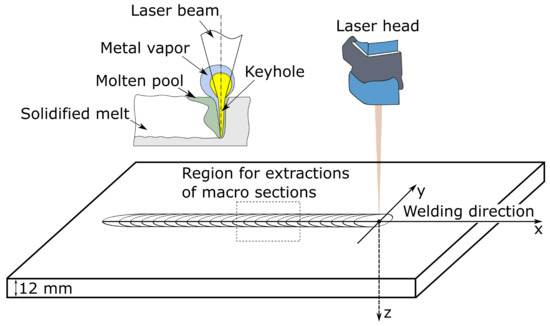
Figure 1.
Schematic of the bead-on-plate laser beam welding process.
Table 2.
Process parameters of the experiments.
2.3. Numerical Modeling
A three-dimensional thermo-fluid dynamics model tracking the free surface deformation by the volume of fluid (VOF) technique was developed for the study of the high power LBW process at high process speeds. The multi-physics model is based on several previous works with some further improvements and adaptions. More details can be obtained from the authors’ previous works [46,47,48,49,50]. Note that only the main physical features of the welding process are formulated concisely in the manuscript; thus the emphasis is on the improvements in the model, especially on the ray tracing approach.
2.3.1. Assumptions
In recent years, the numerical modeling of many industrial and scientific problems has become an inseparable part of their research due to the rapid increase in computational capacity. However, the precise mathematical description of the complex physics behind the high-power LBW process, including numerous strongly coupled, highly-nonlinear interactions between the laser radiation, the vapor phase, the molten metal, and the solid material, remains challenging. Thus, several assumptions and simplifications need to be made in the simulation procedure to allow for feasible computational times. The main assumptions made in the model are the following:
- The molten metal and the gas phases are assumed to be Newtonian and incompressible fluids.
- The flow regimes in the model are considered to be laminar.
- The Boussinesq approximation is used to model the impact of the density deviation on the flow.
2.3.2. Governing Equations
The governing equations describing the multi-physics model in a fixed Cartesian coordinate system are summarized below.
The VOF technique is applied to track the transient deformation of the molten pool free surface and solidified weld seam profile.
• Volume fraction conservation
where denotes the volume fraction of the steel phase in a control volume and is the fluid velocity vector [51].
• Mass conservation
• Momentum conservation
where is the volume-fraction-averaged density, t is the time, p is the fluid pressure, is the volume-fraction-averaged dynamic viscosity, is the gravitational acceleration vector, and is the source term. The source term takes into account the thermal buoyancy due to the variations of the density of the steel with temperature [52]; the deceleration of the flow in the mushy zone, which is related to the inverse of the size of the interdendritic structure [53,54]; the effects of surface tension along the steel-air interface [55]; the evaporation-induced recoil pressure [56]; and the vapor-induced effects, such as stagnation pressure and shear stress on the keyhole surface [43].
• Energy conservation
where is the enthalpy, is the heat conductivity, and is the source term. The source term takes into account the laser heat flux density, the convective and radiative heat transfer, the evaporation loss and the recondensation. Note that the outward as well as the inward convective and radiative heat fluxes due to the high-temperature metal vapor, reaching temperature of up to 6000 , are considered according to [44]. In the present work the range of action for the vapor-induced secondary heat effects was adapted according to the geometrical dimensions of preliminary obtained metallographic cross-sections.
2.3.3. Raytracing Algorithms
A precise description of the laser energy distribution on the keyhole wall is crucial for an accurate calculation of the transient keyhole and weld pool dynamics. A physics-based self-consistent ray-tracing algorithm, rather than an empirical volumetric heat source, is commonly preferred for the description of the multiple reflections and the Fresnel absorptions considered as the key physical aspects of the beam–matter interaction in the LBW process. In the authors’ previous studies, a ray-tracing algorithm, based on the work presented in [40], was implemented in the commercial finite volume method software Ansys Fluent via user-defined functions. Instead of calculating the radiative transfer Equation [57] or the path of Lagrangian photonic parcels [58], the laser beam is divided into 755 sub-rays, which results from discretizing the laser spot in the focal plane by 31 × 31 sub-regions, and each sub-ray is given its own location-dependent energy density and initial incidence angle according to the laser beam profile. Hereby, the laser heat flux density is assumed to have a Gaussian-like axissymetric distribution according to [43]. The temporal and spatial distribution of the laser energy on the keyhole wall can be obtained after calculating the multiple reflections and the Fresnel absorptions of all sub-rays [59].
Since the keyhole profile calculated with the VOF method is not explicit, it may lead to difficulties in determining the exact reflection position of the sub-ray geometrically. Therefore, a compromised criteria is applied in the present study, identifying a cell as a “reflection cell” when the following criteria is satisfied [40]:
where is the distance between the cell center and the incident ray; is the cell size.
It can be seen from Equation (5) that the accuracy of the ray-tracing algorithm is directly determined by the cell size. However, the recommended optimal cell size of [60], which is comparable with the laser spot radius of , has to be chosen for an affordable computational time. This leads to certain inaccuracies, especially when the keyhole front wall is nearly parallel to the laser beam and fluctuates with an amplitude comparable to the cell size, as shown in Figure 2a, where the gray regions represent the steel phase within the cells. The deviations may become unacceptable for high-power LBW of thick sheets at high process speeds due to the higher energy densities, leading to more severe fluctuation of the keyhole wall. Therefore, a local virtual grid refinement algorithm was developed to improve the accuracy of the ray-tracing algorithm [61] without a noticeable increase in the computational intensity; see Figure 2b.
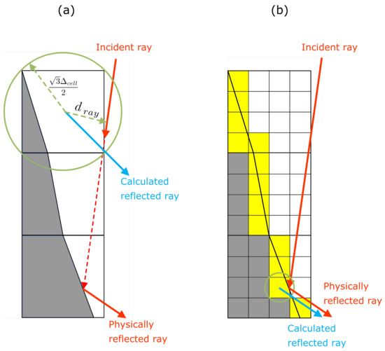
Figure 2.
Schematic of the sub-ray path using a projection of the 3D cells. (a) The standard ray tracing method; (b) the ray tracing with virtual mesh refinement method.
By assuming the free surface to be a piecewise linear interface, the distance between the cell center and the free surface within the cell, (see Figure 3) can be determined uniquely by using the volume fraction of the steel phase and its gradient, , given as [62]. Taking the cell center as the origin and substituting as the maximum, median, and minimum values from , five scalar conditions are obtained, as shown in Figure 3. These can be expressed as:
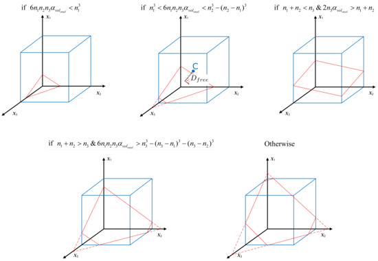
Figure 3.
Calculated distance between the cell center and the free surface within the cell, , depending on the approximated plane of the free surface.
can be calculated analytically or numerically by using Equation (6). Hereby, the free surface within the cell is approximated as:
and once is known, it can be used to determine the virtual cells lying on the free surface.
In the first step of the ray-tracing algorithm, all potential reflection cells are selected by applying the condition defined in Equation (5) and using . Subsequently, the selected cells are further divided into virtual cells with a typical cell size of . The virtual cells on the free surface are identified by Equation (7) and marked in yellow as seen Figure 2b. Note that the cells in Figure 2b marked in gray are the cells excluded from the calculation of the reflection point. In the last step, the reflection point is determined among the selected cells by repeating step one with the virtual mesh cell size .
2.3.4. Boundary Conditions
Following the basic principles of fluid dynamics and assuming the air phase to be inviscid and incompressible, two scalar conditions for the pressure and viscous stress on the steel-air interface are defined:
Note that the surface unit normal is directed into the interior of the steel phase.
The energy boundary condition on the steel-air interface, considering the multiple Fresnel absorption, heat convection, thermal radiation, evaporation, and recondensation, is expressed as:
The boundaries of the air-phase domain were set as pressure outlets and on the bottom of the steel-phase domain, convective heat transfer was considered. The simulation domain was smaller than the real steel sheets to optimize the computational time. Hence, a proper treatment of the boundaries was ensured by utilizing the continuity boundary condition [63]. The boundary conditions are also shown in Figure 4.
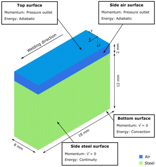
Figure 4.
Boundary conditions of the multi-physics model.
2.3.5. Material Properties
Temperature-dependent material properties were implemented for the simulation of the LBW process. The maximum reachable temperature in the simulation was set to K. The base material was modeled as ferritic phase, whereby for the temperatures above the austenitization temperature, the properties of the austenite phase were used. The phase-specific properties were taken from the literature [64,65,66]; if they were not available, the values for pure iron were taken, due to the close chemical composition (Fe ∼ 98%). The solid–solid phase transformation (ferrite–austenite) was included to the specific heat and the austenite-martensite phase transformation was neglected due to its relatively small amount of latent heat. The thermo-physical material properties are shown in Figure 5. An averaged value of the steel density was calculated for the temperature range of interest between and , giving .
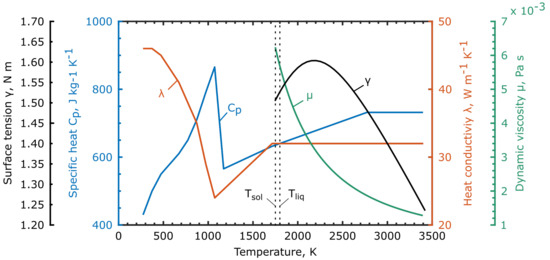
Figure 5.
Thermo-physical material properties for unalloyed steel used in the multi-physics model [64,65,66].
2.3.6. Numerical Setup
The computational domain used in the present study had dimensions of 18 in length, 8 in width, and 12 in thickness; see Figure 4. The domain is uniformly meshed by hexahedral cells of , resulting in a total amount of 189,000 control volumes. An air layer between was defined above the steel sheet (), allowing the tracking of the steel-air interface by the VOF method.
All governing equations were solved with the commercial finite volume method software ANSYS Fluent. A second order upwind scheme was used for the spatial discretization of the momentum and energy conservation equations, and a first-order implicit formulation was applied for the discretization of the transient terms. The pressure-velocity coupling was realized by the PISO scheme and the steel-air interface was reconstructed by the Geo-Reconstruct method.
A high-performance computing cluster with 88 CPU cores at the Bundesanstalt für Materialforschung und –prüfung (BAM) was used for the computation. The averaged computing time was approximately 24 h for 0.25 s real process time.
3. Results
3.1. Process Efficiency and Drilling Speeds
First, the process efficiencies for both welding parameters, given in Table 2, with the different ray tracing algorithms described above are calculated and compared. However, although different welding parameters were used, the line energy was kept equal. A closer look at Figure 6 shows that there are much less fluctuations in the amount of absorbed energy predicted by the standard ray tracing method compared to the virtually improved algorithm, for both low and high process speeds. There were almost constant maximum values of the absorbed laser energy during the simulation with the standard algorithm; see Figure 6a,c. In contrast, the simulation with the virtual mesh refinement does not have clearly pronounced maximum value for the absorbed energy; see Figure 6b,d. Strictly speaking, this means that in the calculations with the virtually refined ray tracing method, more sub-rays are either reaching the keyhole bottom or have been reflected out of it, leading to fluctuations around the averaged value of the absorbed laser energy. Hence, the averaged values of the absorbed amount of laser energy obtained with the improved ray tracing method are slightly lower than those predicted by the standard algorithm. The averaged values at the lower process speed of −1 are 83% and 76% for the standard and virtually refined method, respectively. At the higher process speed of −1, the differences are even smaller, with 83% for the standard and 81% for the virtually refined approach. Note that all calculated process efficiencies lie within the experimental range of measurements at similar process conditions; see, e.g., [67]. Thus, no conclusive statement regarding the physicality and accuracy of the ray tracing algorithms can be given.
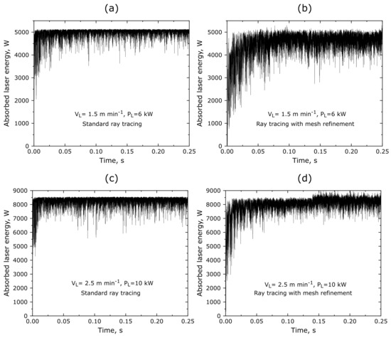
Figure 6.
Calculated process efficiency curves for LBW of 12 mm thick unalloyed sheets with the standard and virtually refined ray tracing algorithms. The corresponding process parameters are given in the sub-figures (a–d).
In the next step, the drilling curves and speeds predicted by the standard and virtually refined ray tracing algorithms are compared and analysed. As seen in Figure 7a, at lower process speed, both algorithms deliver similar results. The penetration depth reached is about and for the standard and virtually refined methods, respectively. Furthermore, the drilling speed in the first 50 of the simulation, estimated from the slopes of the drilling curves, seems to be similar for both ray tracing methods (94 −1 vs. 124 −1). On the other hand, a closer look at the results obtained for LBW at higher process speeds (Figure 7b) shows much bigger differences in the final penetration depth as well as in the drilling speed. The deviation of the penetration depth is about 3 , and the drilling speed is almost two times higher in the simulation utilizing the virtually refined technique (114 −1 vs. 196 −1). This result is surprising, since both welding parameter sets had the same line energies, and the differences of the calculated process efficiencies were negligible from a practical point of view.
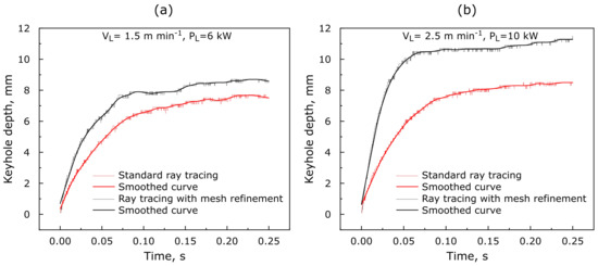
Figure 7.
Comparison of the calculated drilling curves with the standard and virtually refined ray tracing algorithms: (a) −1, , (b) −1, .
In the last step, the accuracy of the numerically obtained penetration depths from both algorithms is validated by comparing them to experimental measurements; see Figure 8. It can be seen from Figure 8a that in the case of modeling LBW at comparatively lower process speed of −1, both ray tracing algorithms deliver results that are close to those from the experiments. It is worth mentioning that although the penetration depth obtained with the standard method is lower than the value predicted by the improved ray tracing algorithm, both values lie within the tolerance range of the experiments. Hereby, the tolerances of the simulation are determined by the half size of the control volumes of . The experimental tolerances on the other hand are obtained by comparing three metallographic cross-sections extracted from the quasi-steady state region of the weld seam, according to Figure 1. In Figure 8b,c exemplary metallographic cross-sections of 12 thick unalloyed steel sheets laser beam welded at −1 and −1, respectively, are shown. As seen in Figure 8a, at the higher process speed of −1, significant differences emerge between the numerically predicted by the standard method and experimentally obtained penetration depths. However, the results obtained with the virtually refined ray tracing algorithm show very good agreement with the measured penetration depth. Hence, it can be concluded that the standard ray tracing technique is well-suited for the computation of the LBW process of thick sheets at lower process speeds. However, the virtually refined ray tracing algorithm seems to provide sufficient accuracy at both low and high welding speed.
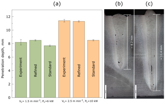
Figure 8.
Calculated and measured penetration depths for LBW of 12 mm thick unalloyed sheets. (a) Comparison between experiment, standard and virtually refined ray tracing algorithms; experimental result for (b) −1, and (c) −1, .
3.2. Correlation between the Energy Distributions in the Keyhole and the Penetration Depth
In order to reveal the physical reasons for the different accuracy of the ray tracing algorithms regarding the predicted penetration depths, the energy distribution in the keyhole is studied in detail for both methods. In Figure 9, the location of the maximum laser energy during LBW at −1 is exemplarily plotted in the time interval between and for the standard and virtually refined algorithm. Note that the maximum value of the absorbed laser energy is used for the analysis since it provides comprehensive information about the keyhole geometry as well. For example, according to the basic principles of the LBW process, the ablation of the front keyhole wall is directly connected with the movement of the maximum laser energy location from the top to the bottom region of the keyhole. Once the the energy is concentrated on the keyhole bottom, the keyhole depth increases, allowing for the deep-penetration LBW [68]. Thus, the ablation process of the front keyhole wall is crucial for the LBW process, especially during welding of thick plates, when it is most pronounced.
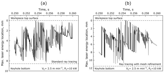
Figure 9.
Temporal distribution of the maximum laser energy location calculated with the (a) standard and (b) virtually refined ray tracing algorithms.
The in-depth analysis of the graphs seen in Figure 9 shows that the maximum laser energy location follows the typical pattern for the LBW process, by first ablating the front keyhole wall and subsequently concentrating on the keyhole bottom, for both ray tracing methods. For instance, during the simulation with the standard algorithm, the ablation process is easily recognized in the time intervals between and , as well as between and ; see Figure 9a. However, the standard algorithm seems to frequently trap the maximum laser energy in the top region, e.g., in the interval between and . Logically, due to this trapping effect, the ablation time of the front wall increases, leading directly to a decrease in the duration time of the maximum energy on the keyhole bottom, thus resulting in a lower penetration depth. In contrast, the trapping effect is not apparent when using the virtually refined method, providing greater accuracy. Additionally, to better visualize the physicality of the ray tracing algorithm, a benchmark was developed and utilized. The benchmark includes a predefined keyhole geometry with typical characteristics for the high-power LBW of thick plates at high process speed, such as deep and narrow profile, an inclined front keyhole wall, and a hump thereon, i.e., a dynamic fluctuation. Both ray tracing algorithms are applied to the predefined keyhole geometry, as shown in Figure 10. With a closer look at Figure 10a, it can be easily seen that the standard algorithm traps most of the laser energy in the hump region. Thus, only a small part of the total laser energy reaches the bottom, resulting in the insufficient penetration depth. However, as seen in Figure 10b, part of the laser beam can pass the hump and directly reach the bottom of the keyhole when the virtually refined raytracing method is applied. Additionally, without the trapping effect part of the laser energy is first reflected to the rear keyhole wall and subsequently reflected to the keyhole bottom. Hence, much more energy is accumulated at the bottom of the keyhole, leading to realistic predictions of the penetration depth.
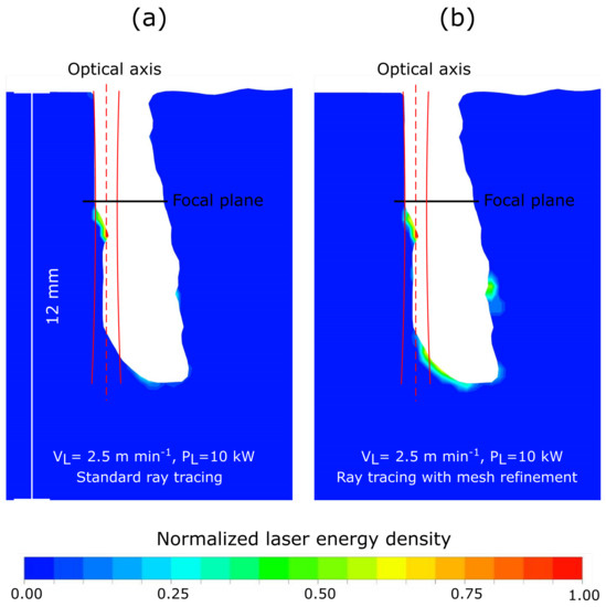
Figure 10.
Distribution of the laser energy calculated with the (a) standard and (b) virtually refined ray tracing algorithms on a predefined keyhole geometry.
It is, however, worth mentioning that the increase in accuracy of the calculated energy distribution within the keyhole can also be achieved by directly using finer mesh, i.e., of the size of the virtual mesh of about . However, such discretization will increase the number of control volumes by approximately 64 times when meshing the computational domain uniformly with hexahedral elements. Additionally, to ensure numerical stability, smaller time steps should be used due to the smaller cell size. Hence, the use of finer discretization remains challenging and unrealistic, even at present time. In contrast, the virtually refined ray tracing technique allows approaching the problem successively and obtaining an accurate solution by almost no increase in the computational intensity.
4. Conclusions
In the current work the plausibility of the well-known and widely used ray tracing algorithms is studied for the high power LBW of thick sheets at different process speeds. The main conclusions drawn based on the obtained results are summarized as follow:
- A three-dimensional transient multi-physics numerical model is developed, allowing for the prediction of the keyhole geometry and the final penetration depth.
- Two ray tracing algorithms are implemented, namely a standard ray-tracing approach and an approach using a virtual mesh refinement for more accurate calculation of the reflection points.
- Both algorithms provide sufficient accuracy for the prediction of the keyhole depth during LBW with process speeds of up to −1.
- The standard algorithm is found to underestimate the penetration depth at process speeds of −1 due to a trapping effect of the laser energy in the top region.
- The virtually refined ray tracing approach results in high accuracy results for both process speeds of −1 and −1.
Author Contributions
Conceptualization: A.A., X.M. and M.B.; Methodology, Software, Validation, Formal analysis, Investigation, Visualization: A.A. and X.M.; Writing—Original Draft Preparation: A.A. and X.M.; Writing—Review & Editing: A.A., X.M., M.B. and M.R.; Supervision, M.B. and M.R.; Project Administration, M.B.; Funding Acquisition, M.B. and M.R. All authors have read and agreed to the published version of the manuscript.
Funding
This work is funded by the Deutsche Forschungsgemeinschaft (DFG, German Research Foundation)—project Nr. 411393804 (BA 5555/5-1) and Nr. 416014189 (BA 5555/6-1).
Conflicts of Interest
The authors declare no conflict of interest. The funders had no role in the design of the study; in the collection, analyses, or interpretation of data; in the writing of the manuscript, or in the decision to publish the results.
References
- Swift-Hook, D.T.; Gick, A.E.F. Penetration welding with lasers. Weld. J. 1973, 52, 492–499. [Google Scholar]
- Zhang, X.; Ashida, E.; Tarasawa, S.; Anma, Y.; Okada, M.; Katayama, S.; Mitzutani, M. Welding of thick stainless steel plates up to 50 mm with high brightness lasers. J. Laser Appl. 2011, 23, 022002. [Google Scholar] [CrossRef]
- Nielsen, S.E. High power laser hybrid welding—Challenges and perspectives. Phys. Procedia 2015, 78, 24–34. [Google Scholar] [CrossRef]
- Katayama, S.; Mizutani, M.; Kawahito, Y.; Ito, S.; Sumimori, D. Fundamental research of 100 kW fiber laser welding technology. In Proceedings of the Lasers in Manufacturing Conference (LiM), Munich, Germany, 22–25 June 2015; pp. 22–25. [Google Scholar]
- Bachmann, M.; Gumenyuk, A.; Rethmeier, M. Welding with high-power lasers: Trends and developments. Phys. Procedia 2016, 83, 15–25. [Google Scholar] [CrossRef]
- Jones, L.P.; Aubert, P.; Avilov, V.; Coste, F.; Daenner, W.; Jokinen, T.; Nightingale, K.R.; Wykes, M. Towards advanced welding methods for the ITER vacuum vessel sectors. Fusion Eng. Des. 2003, 69, 215–220. [Google Scholar] [CrossRef]
- Fang, C.; Song, Y.; Wu, W.; Wei, J.; Zhang, S.; Li, H.; Dolgetta, N.; Libeyre, P.; Cormany, C.; Sgobba, S. The laser welding with hot wire of 316 LN thick plate applied on ITER correction coil case. J. Fusion Energy 2014, 33, 752–758. [Google Scholar] [CrossRef]
- Fang, C.; Xin, J.; Dai, W.; Yang, W.; Wei, J.; Song, Y. 20 kW laser welding applied on the international thermonuclear experimental reactor correction coil case welding. J. Laser Appl. 2020, 32, 022039. [Google Scholar] [CrossRef]
- Kawahito, Y.; Mizutani, M.; Katayama, S. High quality welding of stainless steel with 10 kW high power fibre laser. Sci. Technol. Weld. Join. 2010, 14, 288–294. [Google Scholar] [CrossRef]
- Xu, J.; Rong, Y.; Huang, Y.; Wang, P.; Wang, C. Keyhole-induced porosity formation during laser welding. J. Mater. Process. Technol. 2018, 252, 720–727. [Google Scholar] [CrossRef]
- Zhang, M.J.; Chen, G.Y.; Zhou, Y.; Li, S.C.; Deng, H. Observation of spatter formation mechanisms in high-power fiber laser welding of thick plate. Appl. Surf. Sci. 2013, 280, 868–875. [Google Scholar] [CrossRef]
- Li, S.; Chen, G.; Katayama, S.; Zhang, Y. Relationship between spatter formation and dynamic molten pool during high-power deep-penetration laser welding. Appl. Surf. Sci. 2014, 280, 481–488. [Google Scholar] [CrossRef]
- Bachmann, M.; Avilov, V.; Gumenyuk, A.; Rethmeier, M. Numerical simulation of full-penetration laser beam welding of thick aluminium plates with inductive support. J. Phys. Appl. Phys. 2011, 45, 035201. [Google Scholar] [CrossRef]
- Avilov, V.V.; Gumenyuk, A.; Lammers, M.; Rethmeier, M. PA position full penetration high power laser beam welding of up to 30 mm thick AlMg3 plates using electromagnetic weld pool support. Sci. Technol. Weld. Join. 2012, 17, 128–133. [Google Scholar] [CrossRef]
- Schuster, J. Heißrisse in Schweißverbindungen: Entstehung, Nachweis und Vermeidung; DVS—Verlag: Düsseldorf, Germany, 2004. [Google Scholar]
- Cross, C. On the origin of weld solidification cracking. In Hot Cracking Phenomena in Welds; Springer: Berlin/Heidelberg, Germany, 2005; pp. 3–18. [Google Scholar]
- Bakir, N.; Artinov, A.; Gumenyuk, A.; Bachmann, M.; Rethmeier, M. Numerical simulation on the origin of solidification cracking in laser welded thick-walled structures. Metals 2018, 8, 406. [Google Scholar] [CrossRef] [Green Version]
- Li, L. A comparative study of ultrasound emission characteristics in laser processing. Appl. Surf. Sci. 2002, 186, 604–610. [Google Scholar] [CrossRef]
- Wang, J.; Yu, H.; Qian, Y.; Yang, R. Interference analysis of infrared temperature measurement in hybrid welding. In Robotic Welding, Intelligence and Automation; Springer: Berlin/Heidelberg, Germany, 2011; pp. 369–374. [Google Scholar]
- Artinov, A.; Bakir, N.; Bachmann, M.; Gumenyuk, A.; Na, S.J.; Rethmeier, M. On the search for the origin of the bulge effect in high power laser beam welding. J. Laser Appl. 2019, 31, 022413. [Google Scholar] [CrossRef]
- Saeed, G.; Lou, M.; Zhang, Y.M. Computation of 3D weld pool surface from the slope field and point tracking of laser beams. Meas. Sci. Technol. 2003, 15, 389. [Google Scholar] [CrossRef] [Green Version]
- Song, H.S.; Zhang, Y.M. Three-dimensional reconstruction of specular surface for a gas tungsten arc weld pool. J. Meas. Sci. Technol. 2007, 18, 3751. [Google Scholar] [CrossRef] [Green Version]
- Kim, C.H.; Ahn, D.C. Coaxial monitoring of keyhole during Yb: YAG laser welding. Opt. Laser Technol. 2012, 44, 1874–1880. [Google Scholar] [CrossRef]
- Chenglei, Z.; Xixia, L.; Yi, Z. Coaxial Monitoring of Fiber Laser Butt Welding of Zn-Coated Steel Sheets with an Auxiliary Illuminant. Appl. Laser 2013, 01. Available online: https://en.cnki.com.cn/Article_en/CJFDTotal-YYJG201301016.htm (accessed on 16 August 2021).
- Luo, M.; Shin, Y.C. Estimation of keyhole geometry and prediction of welding defects during laser welding based on a vision system and a radial basis function neural network. Int. J. Adv. Manuf. Technol. 2015, 81, 263–276. [Google Scholar] [CrossRef]
- Seto, N.; Katayama, S.; Matsunawa, A. High-speed simultaneous observation of plasma and keyhole behavior during high power CO2 laser welding: Effect of shielding gas on porosity formation. J. Laser Appl. 2019, 12, 245–250. [Google Scholar] [CrossRef]
- Kawahito, Y.; Uemura, Y.; Doi, Y.; Mizutani, M.; Nishimoto, K.; Kawakami, H.; Tanaka, M.; Fujii, H.; Nakata, K.; Katayama, S. Elucidation of the effect of welding speed on melt flows in high-brightness and high-power laser welding of stainless steel on basis of three-dimensional X-ray transmission in situ observation. Weld. Int. 2017, 31, 206–213. [Google Scholar] [CrossRef]
- Simonds, B.J.; Tanner, J.; Artusio-Glimpse, A.; Williams, P.A.; Parab, N.; Zhao, C.; Sun, T. The causal relationship between melt pool geometry and energy absorption measured in real time during laser-based manufacturing. Appl. Mater. Today 2021, 23, 101049. [Google Scholar]
- Wilson, H.A. On convection of heat. Math. Proc. Camb. Philos. Soc. 1904, 12, 406–423. [Google Scholar]
- Rosenthal, D. Mathematical theory of heat distribution during welding and cutting. Weld. J. 1941, 20, 220–234. [Google Scholar]
- Karkhin, V.A.; Pilipenko, A.Y. Modelling thermal cycles in the weld metal and the heat affected zone in beam methods of welding thick plates. Weld. Int. 1997, 11, 401–403. [Google Scholar] [CrossRef]
- Karkhin, V.A.; Khomich, P.N.; Michailov, V.G. Models for volume heat sources and functional-analytical technique for calculating the temperature fields in butt welding. In Mathematical Modelling of Weld Phenomena; Verlag der Technischen Universitaet Graz: Graz, Austria, 2007; pp. 819–834. [Google Scholar]
- Chukkan, J.R.; Vasudevan, M.; Muthukumaran, S.; Kumar, R.R.; Chandrasekhar, N. Simulation of laser butt welding of AISI 316L stainless steel sheet using various heat sources and experimental validation. J. Mater. Process. Technol. 2015, 219, 48–59. [Google Scholar] [CrossRef]
- Kaplan, A. A model of deep penetration laser welding based on calculation of the keyhole profile. J. Phys. Appl. Phys. 1994, 27, 1805. [Google Scholar] [CrossRef]
- Ki, H.; Mazumder, J.; Mohanty, P.S. Modeling of laser keyhole welding: Part I. Mathematical modeling, numerical methodology, role of recoil pressure, multiple reflections, and free surface evolution. Metall. Mater. Trans. A 2002, 33, 1817–1830. [Google Scholar] [CrossRef]
- Ki, H.; Mazumder, J.; Mohanty, P.S. Modeling of laser keyhole welding: Part II. Simulation of keyhole evolution, velocity, temperature profile, and experimental verification. Metall. Mater. Trans. A 2002, 33, 1831–1842. [Google Scholar] [CrossRef]
- Otto, A.; Koch, H.; Leitz, K.H.; Schmidt, M. Numerical simulations—A versatile approach for better understanding dynamics in laser material processing. Phys. Procedia 2011, 12, 11–20. [Google Scholar] [CrossRef] [Green Version]
- Tan, W.; Bailey, N.S.; Shin, Y.C. Investigation of keyhole plume and molten pool based on a three-dimensional dynamic model with sharp interface formulation. J. Phys. D Appl. Phys. 2013, 46, 055501. [Google Scholar] [CrossRef]
- Pang, S.; Chen, X.; Zhou, J.; Shao, X.; Wang, C. 3D transient multiphase model for keyhole, vapor plume, and weld pool dynamics in laser welding including the ambient pressure effect. Opt. Lasers Eng. 2015, 74, 47–58. [Google Scholar] [CrossRef]
- Cho, J.H.; Na, S.J. Implementation of real-time multiple reflection and Fresnel absorption of laser beam in keyhole. J. Phys. D Appl. Phys. 2006, 39, 5372. [Google Scholar] [CrossRef]
- Cho, W.I.; Na, S.J.; Cho, M.H.; Lee, J.S. Numerical study of alloying element distribution in CO2 laser–GMA hybrid welding. Comput. Mater. Sci. 2010, 49, 792–800. [Google Scholar] [CrossRef]
- Panwisawas, C.; Sovani, Y.; Turner, R.P.; Brooks, J.W.; Basoalto, H.C.; Choquet, I. Modelling of thermal fluid dynamics for fusion welding. J. Mater. Process. Technol. 2018, 252, 176–182. [Google Scholar] [CrossRef]
- Cho, W.-I.; Na, S.-J.; Thomy, C.; Vollertsen, F. Numerical simulation of molten pool dynamics in high power disk laser welding. J. Mater. Process. Technol. 2012, 212, 262–275. [Google Scholar] [CrossRef]
- Muhammad, S.; Han, S.W.; Na, S.J.; Gumenyuk, A.; Rethmeier, M. Study on the role of recondensation flux in high power laser welding by computational fluid dynamics simulations. J. Laser Appl. 2018, 30, 012013. [Google Scholar] [CrossRef]
- Svenungsson, J.; Choquet, I.; Kaplan, A.F. Laser welding process—A review of keyhole welding modelling. Phys. Procedia 2015, 78, 182–191. [Google Scholar] [CrossRef] [Green Version]
- Meng, X.; Bachmann, M.; Artinov, A.; Rethmeier, M. Experimental and numerical assessment of weld pool behavior and final microstructure in wire feed laser beam welding with electromagnetic stirring. J. Manuf. Process. 2019, 45, 408–418. [Google Scholar] [CrossRef]
- Meng, X.; Artinov, A.; Bachmann, M.; Rethmeier, M. Numerical and experimental investigation of thermo-fluid flow and element transport in electromagnetic stirring enhanced wire feed laser beam welding. Int. J. Heat Mass Transf. 2019, 144, 118663. [Google Scholar] [CrossRef]
- Meng, X.; Artinov, A.; Bachmann, M.; Rethmeier, M. Numerical study of additional element transport in wire feed laser beam welding. Procedia CIRP 2020, 94, 722–725. [Google Scholar] [CrossRef]
- Meng, X.; Artinov, A.; Bachmann, M.; Rethmeier, M. Theoretical study of influence of electromagnetic stirring on transport phenomena in wire feed laser beam welding. J. Laser Appl. 2020, 32, 022026. [Google Scholar] [CrossRef]
- Meng, X.; Bachmann, M.; Artinov, A.; Rethmeier, M. The influence of magnetic field orientation on metal mixing in electromagnetic stirring enhanced wire feed laser beam welding. J. Mater. Process. Technol. 2021, 294, 117135. [Google Scholar] [CrossRef]
- Hirt, C.W.; Nichols, B.D. Volume of Fluid (VOF) Method for the Dynamics of Free Boundaries. J. Comput. Phys. 1981, 39, 201–225. [Google Scholar] [CrossRef]
- Faber, T.E. Fluid Dynamics for Physicists; Cambridge University Press: Cambridge, UK, 1995. [Google Scholar]
- Voller, V.R.; Prakash, C. A fixed grid numerical modelling methodology for convection-diffusion mushy region phase-change problems. Int. J. Heat Mass Transf. 1987, 30, 1709–1719. [Google Scholar] [CrossRef]
- Brent, A.D.; Voller, V.R.; Reid, K.T.J. Enthalpy-porosity technique for modeling convection-diffusion phase change: Application to the melting of a pure metal. Numer. Heat Transf. Part A Appl. 1988, 13, 297–318. [Google Scholar]
- Mills, K.C.; Keene, B.J.; Brooks, R.F.; Shirali, A. Marangoni effects in welding. Philos. Trans. R. Soc. Lond. Ser. A Math. Phys. Eng. Sci. 1998, 356, 911–925. [Google Scholar] [CrossRef]
- Semak, V.; Matsunawa, A. The role of recoil pressure in energy balance during laser materials processing. J. Phys. D Appl. Phys. 1997, 38, 2541. [Google Scholar] [CrossRef]
- Khairallah, S.A.; Martin, A.A.; Lee, J.R.; Guss, G.; Calta, N.P.; Hammons, J.A.; Nielsen, M.H.; Chaput, K.; Schwalbach, E.; Shah, M.N.; et al. Controlling interdependent meso-nanosecond dynamics and defect generation in metal 3D printing. Science 2020, 368, 660–665. [Google Scholar] [CrossRef]
- Otto, A.; Vázquez, R.G. Fluid dynamical simulation of high speed micro welding. J. Laser Appl. 2018, 30, 032411. [Google Scholar] [CrossRef]
- Schulz, W.; Simon, G.; Urbassek, H.M.; Decker, L. On laser fusion cutting of metals. J. Phys. D Appl. Phys. 1987, 20, 481–488. [Google Scholar] [CrossRef]
- Cho, W.I.; Na, S.J. Impact of Wavelengths of CO2, Disk, and Green Lasers on Fusion Zone Shape in Laser Welding of Steel. J. Weld. Join. 2020, 38, 235–240. [Google Scholar] [CrossRef]
- Han, S.W.; Ahn, J.; Na, S.J. A study on ray tracing method for CFD simulations of laser keyhole welding: Progressive search method. Weld. World 2016, 60, 247–258. [Google Scholar] [CrossRef]
- Youngs, D.L. Time-dependent multi-material flow with large fluid distortion. Numer. Methods Fluid Dyn. 1982, 24, 273–285. [Google Scholar]
- Meng, X.; Qin, G.; Zong, R. Thermal behavior and fluid flow during humping formation in high-speed full penetration gas tungsten arc welding. Int. J. Therm. Sci. 2018, 134, 380–391. [Google Scholar] [CrossRef]
- Sahoo, P.; Debroy, T.; McNallan, M.J. Surface tension of binary metal-surface active solute systems under conditions relevant to welding metallurgy. Metall. Trans. B 1988, 19, 483–491. [Google Scholar] [CrossRef]
- Mills, K.C. Recommended Values of Thermophysical Properties for Selected Commercial Alloys; Woodhead Publishing: Shaxton, UK, 2002. [Google Scholar]
- ESI Group. Material Database; ESI Group: Paris, France, 2009. [Google Scholar]
- Kawahito, Y.; Matsumoto, N.; Abe, Y.; Katayama, S. Relationship of laser absorption to keyhole behavior in high power fiber laser welding of stainless steel and aluminum alloy. J. Mater. Process. Technol. 2011, 211, 1563–1568. [Google Scholar] [CrossRef]
- Wang, Y.; Jiang, P.; Zhao, J.; Geng, S. Effects of energy density attenuation on the stability of keyhole and molten pool during deep penetration laser welding process: A combined numerical and experimental study. Int. J. Heat Mass Transf. 2021, 176, 121410. [Google Scholar] [CrossRef]
Publisher’s Note: MDPI stays neutral with regard to jurisdictional claims in published maps and institutional affiliations. |
© 2021 by the authors. Licensee MDPI, Basel, Switzerland. This article is an open access article distributed under the terms and conditions of the Creative Commons Attribution (CC BY) license (https://creativecommons.org/licenses/by/4.0/).