Application of Machine Learning Algorithms and SHAP for Prediction and Feature Analysis of Tempered Martensite Hardness in Low-Alloy Steels

Abstract

The tempering of low-alloy steels is important for controlling the mechanical properties required for industrial fields. Several studies have investigated the relationships between the input and target values of materials using machine learning algorithms. The limitation of machine learning algorithms is that the mechanism of how the input values affect the output has yet to be confirmed despite numerous case studies. To address this issue, we trained four machine learning algorithms to control the hardness of low-alloy steels under various tempering conditions. The models were trained using the tempering temperature, holding time, and composition of the alloy as the inputs. The input data were drawn from a database of more than 1900 experimental datasets for low-alloy steels created from the relevant literature. We selected the random forest regression (RFR) model to analyze its mechanism and the importance of the input values using Shapley additive explanations (SHAP). The prediction accuracy of the RFR for the tempered martensite hardness was better than that of the empirical equation. The tempering temperature is the most important feature for controlling the hardness, followed by the C content, the holding time, and the Cr, Si, Mn, Mo, and Ni contents.

1. Introduction

The tempering of low-alloy steels involves the control of their mechanical properties through ε-martensite and carbide formation, dislocation recovery, carbide spheroidization, and recrystallization [1,2,3,4,5,6]. It is important to use apposite tempering to meet the property requirements of industrial use. Empirical equations for adjusting the hardness in tempered low-alloy steels have been proposed. Hollomon and Jaffe proposed tempering parameters comprising the tempering temperature and holding time to predict the hardness of tempered martensite. These equations are given by [1]:

$$TP=T\left(\log t+C\right),$$

(1)

$$TMH=\left(1542.97-\frac{25.31}{X_c}\right)·\exp \left(-1.23\times {10}^{-4}TP\right)$$

(2)

where TP is the tempering temperature in Kelvin, t is the holding time in hours for isothermal conditions, C is a constant, TMH is the tempered martensite hardness, and X_c is the amount of carbon in weight percent. The equations effectively explain the effect of the tempering temperature and holding time. The hardness of the tempered martensite varies with the alloy elements. However, this hardness variation cannot be accurately estimated by Equation (2). Kang and Lee proposed a composition-dependent tempering parameter given as [2]

$$TP=T\left(\log t+\left(k_0+\sum _i{k}_i{X}_i\right)\right)$$

(3)

where k₀ is a constant, k_i is the coefficient of element i, and X_i is the amount of alloying element i in weight percent. k₀, k_c, k_Mn, k_Si, k_Ni, k_Cr, and k_Mo were 17.396, −6.661, −1.604, −3.412, −0.248, −1.112, and −4.355, respectively [2]. It has been reported that these optimal $k_i$ values were determined from over 1900 experimental data and revealed the fact that the change of activation energy related to tempering is associated with chemical composition. This equation makes it possible to evaluate the hardness variations of the tempered low-alloy steel with the tempering temperature, holding time, and alloy composition. These equations sufficiently explain the hardness of the tempered martensite. However, it is still important to confirm the importance of each parameter to the hardness of tempered martensite and to improve the accuracy of the equation to reduce the prediction error.

Machine learning algorithms are intensive methods for improving prediction accuracy. They can predict the target values more accurately than classical alloy modeling methods without a trial-and-error process, which requires considerable time, cost, and effort. Such algorithms include random forest regression (RFR), support vector regression (SVR), k-nearest neighbors (kNN), and artificial neural networks (ANN). These algorithms are widely used to predict target parameters such as the yield strength, hardness, and thermal properties in material science [7,8,9,10,11,12,13,14]. For instance, Zhang et al. predicted the mechanical properties of a nonequiatomic high-entropy alloy using an ANN and an SVR [7]. Narayana et al. predicted the mechanical properties of 20Cr-20Ni-0.4C steels over a wide range of temperatures using an ANN [8]. However, the analysis of machine learning models to confirm how they work remains a challenge. Shapley additive explanations (SHAP) have been used to study the mechanisms of trained machine learning algorithms [15,16,17]. Yan et al. evaluated the importance of input features and how they affect the corrosion rate of low-alloy steels using SHAP [15]. This analysis opened the way to the evaluation of the machine learning algorithm mechanisms, which were previously regarded as black boxes.

In this study, we propose the use of machine learning algorithms to improve prediction accuracy and investigate how the tempering temperature, holding time, and alloy composition affect the tempered martensite hardness. We collected a dataset containing the composition, tempering temperature, and holding time of low-alloy steels from the literature. SHAP were then used to assess the trained machine learning mechanisms.

2. Data Collection

Datasets for low-alloy steels were collected from 1926 utilizable datasets from the literature [2]. The datasets consisted of compositions containing six elements (C, Mn, Si, Ni, Cr, and Mo), tempering features such as the tempering temperature and holding time, and the Vickers hardness (HV). The ranges of the compositions, tempering features, and HV are listed in

Table 1. Range of the compositions (wt.%), tempering temperature (°C), holding time (s), and HV in the dataset used in this study.

	Minimum	Maximum	Average	Deviation
C	0.12	1.15	0.45	0.21
Mn	0.00	1.75	0.65	0.32
Si	0.00	0.90	0.24	0.17
Ni	0.00	3.50	0.26	0.71
Cr	0.00	2.00	0.20	0.38
Mo	0.00	0.50	0.06	0.11
Tempering temperature	145	716	444	160
Holding time	30	3,500,000	68,665	344,146
Hardness (HV)	105	899	395	144

.

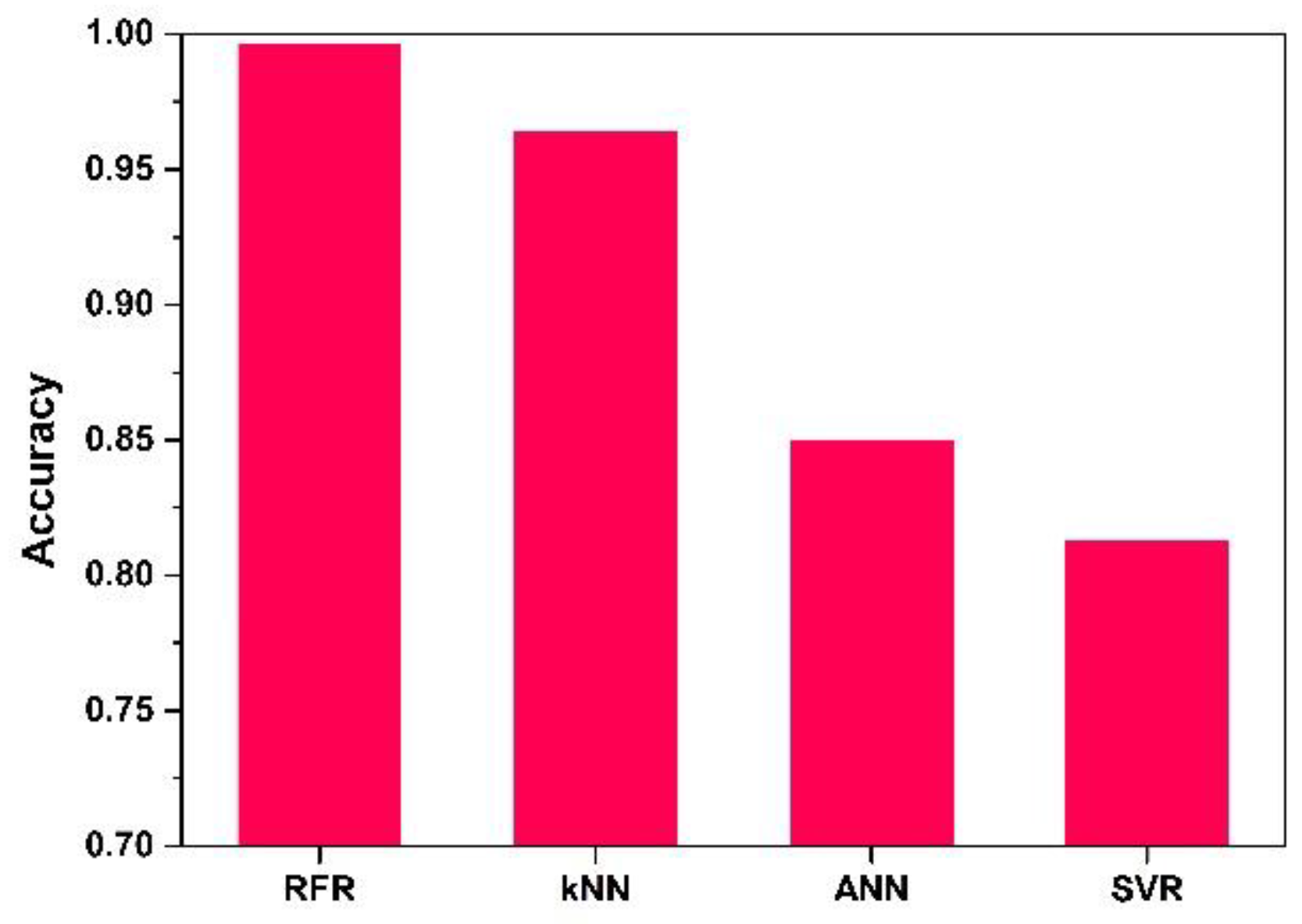
3. Machine Learning Training

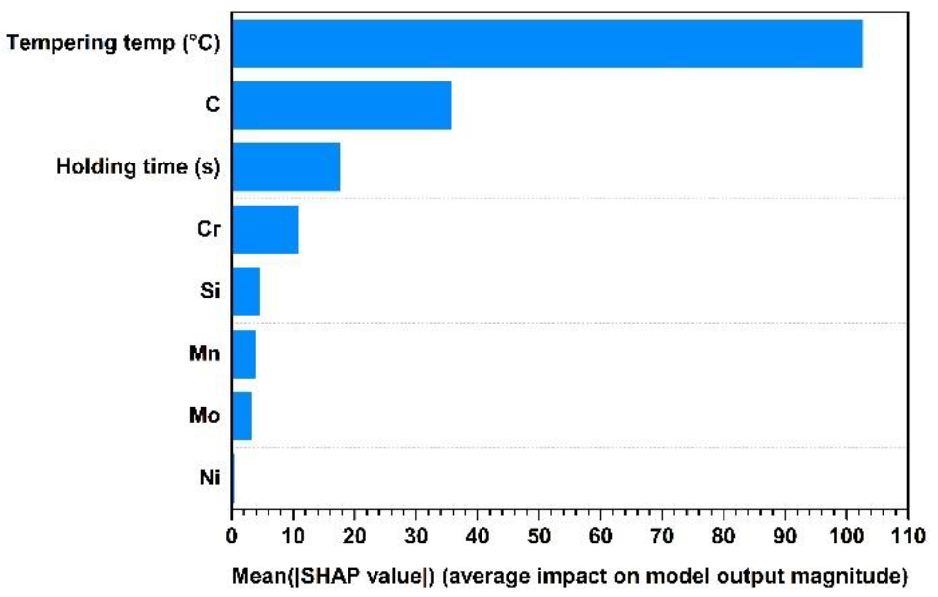
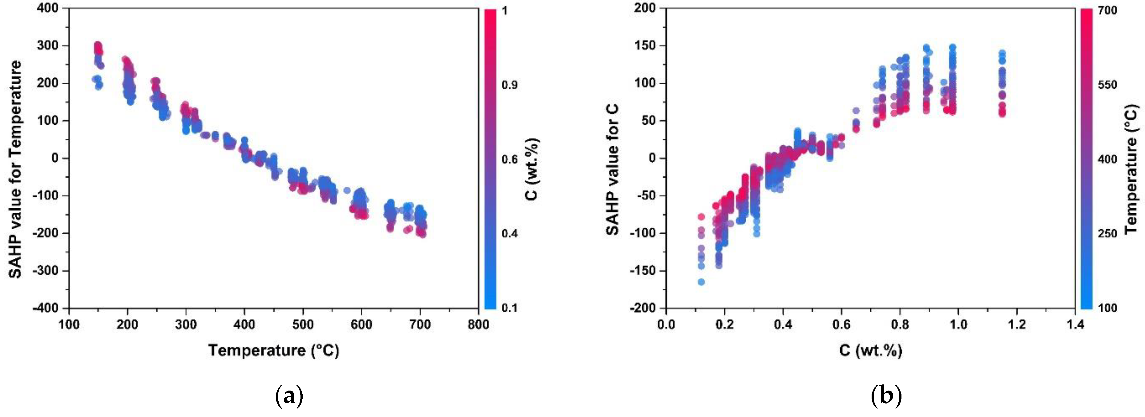
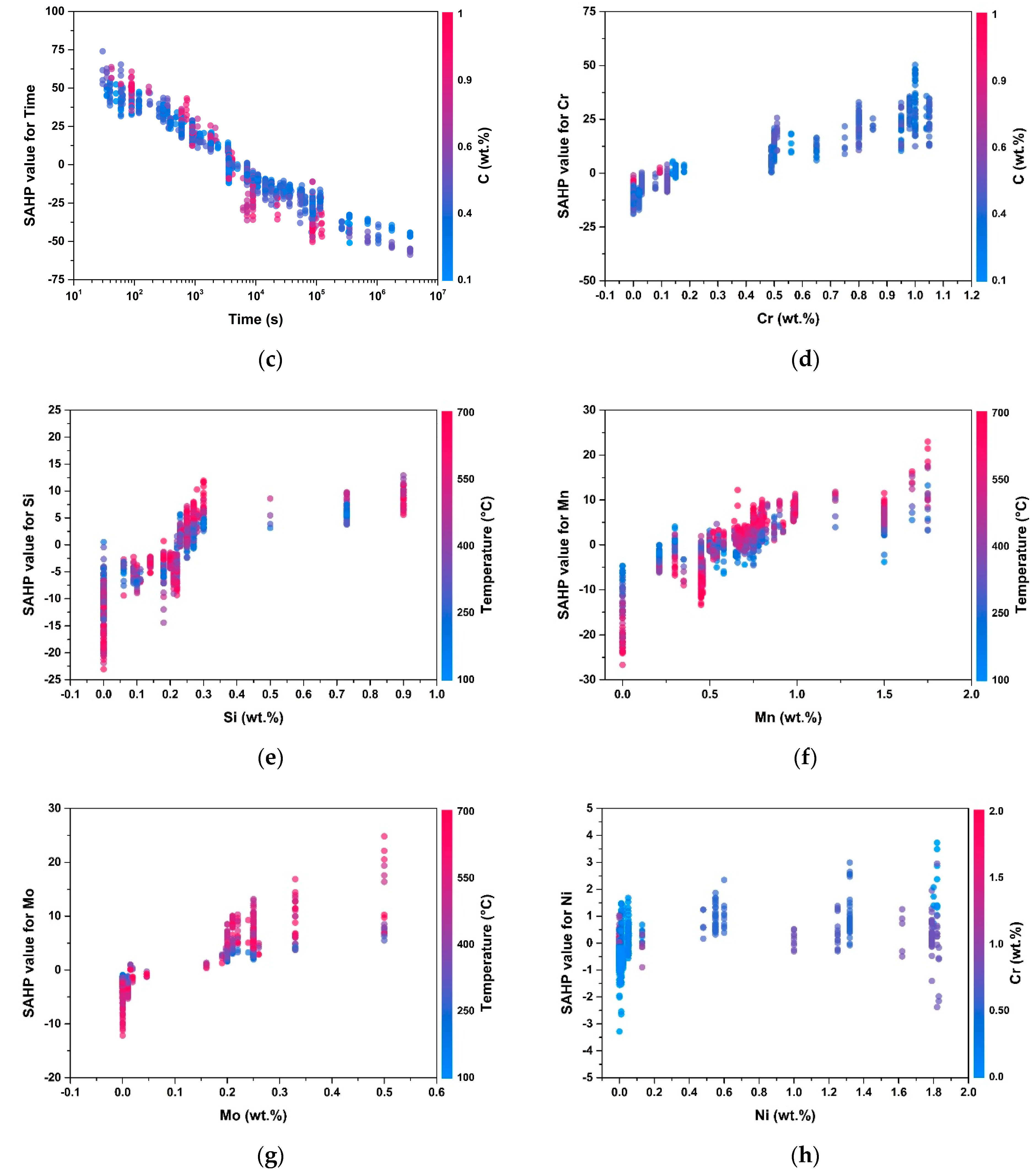
To predict the HV, the ANN, SVR, kNN, and RFR were employed. The ANN learning algorithm searches for the optimal weight and bias features to explain the relationship between the input and target features [18]. The main hyperparameters in ANN learning are the optimizer, activation function, number of layers, and number of nodes. The ANN was trained with the number of layers varied from 1 to 2, the number of neurons from 1 to 100, and the learning rate to 0.0001, 0.0005, 0.001, 0.005, 0.01, 0.05, and 0.1. Deep learning, which has over three hidden layers, is typically used with tens of thousands of data. In this study, we trained the ANN with 1 or 2 layers, which was enough to deal with the total of 1926 datasets efficiently and accurately. In addition, we used root mean squared propagation (RMSprop) as the optimizer, the rectified linear unit (ReLU) as the activation function for the hidden layers, and the linear transfer function (purelin) as the activation function for the output layer. The datasets of the ANN were divided into proportions of 70%, 15%, and 15% for training, validation, and testing, respectively. The SVR algorithm was trained to minimize the weight and satisfy the constraints given by [19]:

$$minimize \frac{1}{2}{\Vert W\Vert }^2+\mathrm{C}{\sum }_{i=1}^l({\xi }_i+{\xi }_i^{\ast }),$$

(4)

$$subject to \{\begin{array}{c}{y}_i-WX-b\le \epsilon +{\xi }_i\\ WX+b-y_i\le \epsilon +{\xi }_i^{\ast }\\ {\xi }_i,{\xi }_i^{\ast }\ge 0\end{array},$$

(5)

where W is the weight matrix, C is a constant, ${\xi }_i$ and ${\xi }_i^{\ast }$ are the soft margins, X is the matrix of input values, b is a constant, and $\epsilon$ is the error. The values of C and $\epsilon$ affect the SVR performance. The SVR was trained with $\epsilon$ set to 0.0001, 0.0005, 0.001, 0.005, 0.01, 0.05, and 0.1. We set C to 100 and used a radial basis kernel with a constant value of 0.1. The kNN algorithm predicts the target value using the k-nearest values [20]. The performance of the kNN varies with the value of k. The kNN algorithm was trained with k values ranging from 1 to 20. The RFR consists of a multitude of decision trees [21,22]. The RFR trains k decision trees and takes the average value. The performance of the RFR is affected by the number of decision trees. The RFR was trained using 10 to 100 decision trees. The datasets for the SVR, kNN, and RFR algorithms were split into 80% for training and 20% for validation, respectively. R² was used to assess the predictive accuracy. The R² value is given by:

$$R^2={\left(\frac{\sum \left[\left(x_i-\overline{x}\right)\left(y_i-\overline{y}\right)\right]}{\sqrt{{\left[\sum \left(x_i-\overline{x}\right)\right]}^2\ast {\left[\sum \left(y_i-\overline{y}\right)\right]}^2}}\right)}^2$$

(6)

where $x$ and $y$ are the measurement and predicted target values, respectively, and $\overline{x}$ and $\overline{y}$ their arithmetic means. The training processes and algorithm assessment were performed using TensorFlow Version 2.0, Google brain team, Mountain View, CA, USA and the scikit-learn Version 0.23.1 module in Python Version 3.7, Python software foundation, Fredericksburg, VA, USA.

4. SHAP Method

For a simple model such as linear regression, the best explanation is often the model itself. However, it is difficult to explain how complex models such as machine learning models work and how the input values affect the target values. The SHAP, which is based on game theory and local explanations, can explain the relationship between the inputs and targets using the Shapley value. The Shapley value can be expressed as [23,24]:

$${\varphi }_i={\displaystyle \sum }_{S\subseteq F\backslash \left\{i\right\}}\frac{\left|S\right|!\left(\left|F\right|-\left|S\right|-1\right)}{\left|F\right|!}\left(v_{S{\displaystyle \cup }\left\{i\right\}}\left(x_{S{\displaystyle \cup }\left\{i\right\}}\right)-v_S\left(x_S\right)\right)$$

(7)

where ${\varphi }_i$ is the Shapley value of the ith input value, $S$ is the set of input values with the ith input value excluded, $\left|S\right|$ is the magnitude of S (for example, $S=\left\{x_1, x_2, \dots , x_{i-1}, x_{i+1}, \dots , x_{n-1}, x_n\right\}$ and $\left|S\right|=n-1)$, F is the set of input values, and $v\left(x\right)$ is calculated based on the marginal contribution of the input values. The explanation model of the linear function of the Shapley value is given by:

$$v\left(z^{\prime }\right)=g\left(z^{\prime }\right)={\varphi }_0+{\displaystyle \sum }_{i=1}^M{\varphi }_i{z}_i^{\prime }$$

(8)

where $z_i^{\prime }\in {\left\{0, 1\right\}}^M$ and M is the number of input values. $z_i^{\prime }$ is 1 when the ith input value is observed and 0 otherwise. The value of the explanation model demonstrates how the model works. For example, if we need a Shapley value of C, we calculate $v\left(x\right)$ with the whole data and $v\left(x\right)$ except the C data. Then, we calculate ${\varphi }_C$. The Shapley value makes it possible to evaluate the average influence of the input value on the target value.

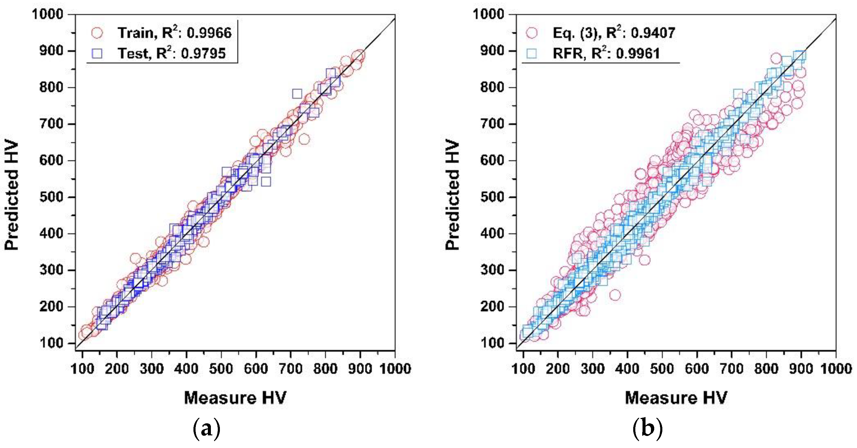
5. Results and Discussion

The machine learning algorithms with the best R² values were selected. Figure 1 shows the accuracy of the selected machine learning algorithms with the training dataset.

RFR exhibited the best R² value of 0.9966. The second best model was kNN, which had an R² value of 0.9648. The ANN and SVR had R² values of less than 0.9. The average learning time for the ANN was 103.8 s, whereas that for the other algorithms was just a few seconds. The selected RFR algorithm consisted of 30 trees. The kNN algorithm had the k value of k = 4 for the HV. The structure of the ANN algorithm was 9-71-1. The learning rate of 0.01 was used in the selected ANN. ε = 0.01 in the selected SVR. Based on the R² values, we chose the RFR for HV prediction. Figure 2a shows the performance of the RFR for the test datasets that were not used for training. The accuracy was 0.9795. This demonstrates that the RFR predictions were reliable and that the RFR was successfully trained. The R² values for the test datasets were 0.9492, 0.8474, and 0.5344 for kNN, the ANN, and the SVR, respectively. Figure 2b shows the performance of Equation (3) and the RFR. The RFR showed a higher accuracy (R² = 0.9961) than Equation (3) (R² = 0.9407). This result indicates that the RFR predicted HV more accurately.

Figure 3 shows the influence of each feature. We calculated the absolute Shapley value of each input value. Then, we averaged it. Therefore, Mean (|SHAP|) indicates the average absolute magnitude of the influence of each input value on HV. The tempering temperature had the greatest influence on the HV, followed by the C content, the holding time, and the contents of Cr, Si, Mn, Mo, and Ni.

Figure 4 shows the average influence of each variation on hardness. Figure 4a shows the effect of the tempering temperature on the HV. Carbon was chosen as a color legend. To make the plot, we calculated the Shapley values at each tempering temperature the with RFR and confirmed the effect of each variation, which mostly related to tempering temperature. Hence, we can say if the tempering temperature increases, HV decreases on average. For the same tempering temperature, the C content is the most effective value to control the HV. Speich et al. proposed that the tempering process can be divided into four stages according to the tempering temperature. The first stage occurs at temperatures between room temperature and 250 °C. In this stage, carbon segregation (<0.2 wt.% C) and ε-carbide precipitation (>0.2 wt.% C) occur. The tempering progresses to the second stage at temperatures between 230 and 300 °C. At this stage, the retained austenite decomposes. The third stage takes place between 200 and 300 °C. At this stage, rod-shaped carbide is precipitated at the austenite grain boundaries, the martensite lath boundaries, the boundaries between ε-carbide and the matrix, and the twin boundaries. The fourth stage occurs between 300 and 600 °C. At this stage, dislocation recovery and Fe₃C spheroidizing occur. Above 600 °C, the crystal structure recrystallizes and Fe₃C coarsening occurs [3,4,5,6]. The HV is decreased according to the four stages of tempering. The tempering temperature effect in the RFR reflects this process.

Figure 4b shows the effect of C on the HV. The HV is enhanced with the increase in the C content. The HV is influenced by several factors, including (1) the restriction of the dislocation movement by C atoms located at interstitial sites, (2) the increase in ε-carbide transformation at tempering temperatures between room temperature and 250 °C, and (3) the decrease in the frequency of auto-tempering due to the decline in the martensite starting temperature. Figure 4a,b show the relationship between the C content and the tempering temperature. At tempering temperatures between 100 and 300 °C, the HV is enhanced when the C content increases. In this range of temperatures, ε-carbide and rod-shaped carbide are precipitated. The amount of carbide increases with the C content, leading to the enhancement of the HV. However, between 400 and 700 °C, the HV is reduced by an increase in the C content. This reduction may be due to the decrease in the recrystallization temperature of the low-carbon alloy. A larger C content increases the density of Fe₃C, which fixes the ferrite boundaries. The earlier occurrence of recrystallization in the low-carbon alloy compared to the high-carbon alloy results in a finer grain in the low-carbon alloy. In contrast, in the high-carbon alloy, spheroidal Fe₃C is formed, and dislocations are recovered. At a large C content, recrystallization is inhibited by the pinning action of carbides on the boundaries. The recrystallization temperature of the low-C alloy is lower than that of the high-C alloy [6].

Figure 4c shows the effect of the holding time on the HV. A longer tempering holding time provides sufficient time for alloy elements to diffuse in the steel alloy. Hence, the tempering process proceeds sufficiently. Figure 4d–h shows the effects of the alloy elements. All the elements improve the HV. Cr and Mo enhance the HV through the formation of carbide, which is harder than Fe₃C. Si improves the stability of ε-carbide by retarding the nucleation and growth of Fe₃C [6]. Mn has been reported to delay the appearance of martensitic to a higher temperature and to make the carbide smaller and more numerous. The HV is hardly affected by Ni [3].

6. Conclusions

In this study, the use of the RFR to predict the HV of low-alloy steels was proposed. The RFR algorithm was trained using the tempering temperature, holding time, and the amounts of added alloying elements C, Mn, Si, Ni, Cr, and Mo. The RFR exhibited a larger improvement in the accuracy of the predicted hardness compared to the composition-dependent empirical equation. The effect of each feature on the RFR was evaluated using the SHAP value. The HV decreased as the tempering temperature and holding time increased and increased as the amount of added alloying composition increased. The most important feature affecting the HV was the tempering temperature, followed by the C content, the holding time, and the Cr, Si, Mn, Mo, and Ni contents.

References

1. Hollomon, J.H.; Jaffe, L.D. Time-temperature relations in tempering steel. Trans. AIME 1945, 162, 223–249. [Google Scholar]
2. Kang, S.; Lee, S.-J. Prediction of Tempered Martensite Hardness Incorporating the Composition-Dependent Tempering Parameter in Low Alloy Steels. Mater. Trans. 2014, 55, 1069–1072. [Google Scholar] [CrossRef] [Green Version]
3. Grange, R.A.; Hribal, C.R.; Porter, L.F. Hardness of Tempered Martensite in Carbon and Low-Alloy Steels. Metall. Trans. A 1977, 8A, 1775–1785. [Google Scholar] [CrossRef]
4. Materkowski, J.P.; Krauss, G. Tempered Martensite Embrittlement in SAE 4340 Steel. Matall. Trans. A 1979, 10A, 1643–1651. [Google Scholar] [CrossRef]
5. Speich, G.R.; Leslie, W.C. Tempering of Steel. Metall. Trans. 1972, 3, 1043–1054. [Google Scholar] [CrossRef]
6. Bhadeshia, H.; Honeycombe, R. Steels: Microstructure and Properties, 3rd ed.; Butterworth-Heinemann: Oxford, UK, 2006; pp. 231–262. [Google Scholar]
7. Zhang, L.; Qian, K.; Schuller, B.W.; Shibuta, Y. Prediction on Mechanical Properties of Non-Equiatomic High-Entropy Alloy by Atomistic Simulation and Machine Learning. Metals 2021, 11, 922. [Google Scholar] [CrossRef]
8. Narayana, P.L.; Kim, J.H.; Maurya, A.K.; Park, C.H.; Hong, J.-K.; Yeom, J.-T.; Reddy, N.S. Modeling Mechanical Properties of 25Cr-20Ni-0.4C Steels over a Wide Range of Temperatures by Neural Networks. Metals 2020, 10, 256. [Google Scholar] [CrossRef] [Green Version]
9. Maurya, A.K.; Narayana, P.L.; Kim, H.I.; Reddy, N.S. Correlation of Sintering Parameters with Density and Hardness of Nano-sized Titanium Nitride reinforced Titanium Alloys using Neural Networks. J. Korean Powder Metall. Inst. 2020, 27, 1–8. [Google Scholar] [CrossRef]
10. Jeon, J.; Seo, N.; Kim, H.-J.; Lee, M.-H.; Lim, H.-K.; Son, S.B.; Lee, S.-J. Inverse Design of Fe-based Bulk Metallic Glasses Using Machine Learning. Metals 2021, 11, 729. [Google Scholar] [CrossRef]
11. Zhang, Y.; Xu, X. Lattice Misfit Predictions via the Gaussian Process Regression for Ni-Based Single Crystal Superalloys. Met. Mater. Int. 2021, 27, 235–253. [Google Scholar] [CrossRef]
12. Park, C.H.; Cha, D.; Kim, M.; Reddy, N.S.; Yeom, J.-T. Neural Network Approach to Construct a Processing Map from a Non-linear Stress-Temperature Relationship. Met. Mater. Int. 2019, 25, 768–778. [Google Scholar] [CrossRef]
13. Lee, W.; Lee, S.-J. Prediction of Jominy Curve using Artificial Neural Network. J. Korean Soc. Heat Treat. 2018, 31, 1–5. [Google Scholar]
14. Schmidt, J.; Marques, M.R.G.; Botti, S.; Marques, M.A.L. Recent advances and applications of machine learning in solid-state materials science. Comput. Mater. 2019, 5, 1. [Google Scholar]
15. Yan, L.; Diao, Y.; Lang, Z.; Gao, K. Corrosion rate prediction and influencing factors evaluation of low-alloy steels in marine atmosphere using machine learning approach. Sci. Technol. Adv. Mat. 2020, 21, 359–370. [Google Scholar] [CrossRef] [Green Version]
16. Parsa, A.B.; Movahedi, A.; Taghipour, H.; Derrible, S.; Mohammadian, A. Toward safer highways, application of XGBoost and SHAP for real-time accident detection and feature analysis. Accid. Anal. Prev. 2020, 136, 105405. [Google Scholar] [CrossRef] [PubMed]
17. Lundberg, S.M.; Nair, B.; Vavilala, M.S.; Horibe, M.; Eisses, M.J.; Adams, T.; Liston, D.E.; Low, D.K.-W.; Newman, S.-F.; Kim, J.; et al. Explainable machine-learning predictions for the prevention of hypoxaemia during surgery. Nat. Biomed. Eng. 2018, 2, 749–760. [Google Scholar] [CrossRef] [PubMed]
18. Asgharzadeh, A.; Asgharzadeh, H.; Simchi, A. Role of Grain Size and Oxide Dispersion Nanopaticles on the Hot Deformation Behavior of AA6063: Experimental and Artificial Neural Network Modeling Investigations. Mat. Mater. Int. 2021, 29. [Google Scholar] [CrossRef]
19. Smola, A.J.; Schölkopf, B. A tutorial on support vector regression. Stat. Comput. 2004, 14, 199. [Google Scholar] [CrossRef] [Green Version]
20. Cover, T.; Hart, P. Nearest Neighbor Pattern Classification. IEEE Trans. Inf. Theory 1967, 13, 21. [Google Scholar] [CrossRef]
21. Murthy, S.K.; Kasif, S.; Salzberg, S. A System for Induction of Oblique Decision Trees. J. Artif. Intell. Res. 1994, 2, 1. [Google Scholar] [CrossRef]
22. Wang, Q.R.; Suen, C.Y. Analysis and Design of a Decision Tree Based on Entropy Reduction and Its Application to Large Character Set Recognition. IEEE Trans. Inf. Theory 1984, 6, 406. [Google Scholar] [CrossRef] [PubMed]
23. Lundberg, S.M.; Lee, S.-I. A Unified Approach to Interpreting Model Predictions. In Proceedings of the 31st International Conference on Neural Information Processing Systems, Long Beach, CA, USA, 4 December 2017; pp. 4768–4777. [Google Scholar]
24. Shapley, L.S. Notes on the N-Person Game II: The Value of an N-Person Game; Technical Report for U.S. Air Force; Rand Corporation: Santa Monica, CA, USA, August 1951. [Google Scholar]
Figure 1. Accuracy of the machine learning algorithms with the training dataset. RFR: random forest regression. kNN: k-nearest neighbors. ANN: artificial neural network. SVR: support vector regression.
Metals 11 01159 g001
Figure 2. Comparison between predicted and measured HV (Vickers hardness). (a) Validation of the RFR algorithm; (b) the performance of the RFR and Equation (3).
Metals 11 01159 g002
Figure 3. The importance of each feature to the HV based on the SHAP (Shapley additive explanations) analysis.
Metals 11 01159 g003
Figure 4. Impact of the input features, which are (a) tempering temperature, (b) C, (c) tempering time, (d) Cr, (e) Si, (f) Mn, (g) Mo, and (h) Ni, on HV.
Metals 11 01159 g004aMetals 11 01159 g004b