Abstract
This work is devoted to the electron temperature variation in metals through interaction with femtosecond laser pulses. Our study was inspired by the last mathematical breakthroughs regarding the exact analytical solutions of the heat equation in the case of flash laser-matter interaction. To this purpose, the classical Anisimov’s two temperature model was extended via the 3D telegraph Zhukovsky equation. Based upon this new approach, the computational plots of electron thermal fields during the first laser pulse interaction with a gold surface were inferred. It is shown that relaxation times and coupling factors over electron thermal conductivities (g/K) govern the interaction between the laser pulse and metal sample during the first picoseconds. The lower the factor g/K, the higher the electron temperature becomes. In contrast, the lower the relaxation time, the lower the electron temperature.
1. Introduction
During ultrashort laser pulse interaction with metals, the heat transfer proceeds in two steps. First, energy absorption occurs via photon–electron interactions, followed by the return of excited electrons to the initial state, lasting for a few femtoseconds. Next, the energy is redistributed from electrons to the lattice by electron–phonon interactions for a few picoseconds, followed by thermalization (i.e., the heat is dissipated, and the lattice reaches thermal equilibrium) [1].
The two temperature model (TTM) can predict the electron and lattice temperatures during the interaction of ultrashort laser pulses (<10 ps) with matter [2]. The model is, however, limited to low laser fluences [3]. Recently, the Zhukovsky theories were successfully extended to TTM [4] at ns and fs scales.
We herewith report on the development and application of a modified TTM [5] to describe the thermal field interaction of femtosecond laser radiation with metals during the first pulse. Standard TTM was combined with a very powerful and new mathematical concept in order to introduce an advance mathematical approach of TTM [5,6,7,8,9]. The novelty of this approach is given by the fact that this is somehow totally the opposite of the existing ones. Up to now, the TTM approached the laser–matter interaction from quantum or semi-classical points of view, but always based on the classical solving of heat equation. In our case, we treated the interaction classically and solved the heat equation using quantic operators.
2. Theoretical Model
Laser radiation-solid interaction is generally well described by the Maxwell–Schrödinger theory combined with numerical methods [10,11]. The authors in [12] developed the formalism of TTM (one for phonons and one for electrons) in laser–metal interaction in detail. For ultrashort pulses, one has two almost decoupled equations because the electron temperature during the first femtoseconds is much higher than the lattice temperature. One may write for electron temperature:
where is the electron temperature depending on x, y, z Cartesian spatial coordinates; t is the time; thermal diffusivity of target; K is the electron thermal conductivity; ci is the specific heat of the electron; and ρ is the mass density of the metallic target, respectively. Q stands for the “source term” of the heat equation and g is the electron-phonon coupling factor.
For lattice temperature, in the case of the first laser pulse, one gets:
It is worth mentioning that in what follows, T is the relative temperature rather than the absolute temperature.
The model should be further connected with Zhukovsky mathematical formalism. To this purpose, the “source term” was introduced, corresponding to temperature at t = 0.
One can further proceed to generalize TTM using the Cattaneo–Vernote equation instead of a Fourier one. A reasonable question is whether the Fourier equation is “strong” enough for this purpose. The answer is that the Cattaneo equation takes into account the “relaxation times” and consequently is appropriate for the characterization of ultrafast thermal behavior. This is precisely not the case of the Fourier equation, which considers an infinite thermal wave speed that is against the special theory of relativity [13].
Accordingly, Equation (1) is generalized to the following Cattaneo–Vernote type equation:
The “source term” is, in this case:
where is the relaxation time for laser–metal interaction, and I is the laser intensity. Equation (4) associates the two models. From a mathematical point of view, the “source term” in the “classical” heat equation is replaced by the initial condition in Equation (4) to describe a single interaction of an ultra-short pulse. The solution of Equations (3) and (4) is [6]:
where are heat operators [6].
One has:
where are Hermite polynomials of order m and n, respectively; R is the target reflectivity; is the optical penetration depth into the target; is the ballistic length; F is the laser fluence; and w is the 1/e radius of the laser spot, while is the maximum penetration length after one laser pulse.
We can rewrite Equation (6) for one single transverse mode, as follows ():
By consequence:
where
One may easily calculate the electron temperature using as input Equation (5) and Equations (8)–(11). Based upon from the Zhukovsky definition of heat operators [2], one further gets:
with .
3. Simulations
Our simulations describe the interaction of a top-hat fs pulse generated by a Ti–sapphire laser source (λ = 760 nm, = 100 fs) with an Au target (δ = 20 nm, = 100 nm), K = 315 W/mK, ci = 2.1 × 10⁴ J/(m3K), and g = 2.1 × 10¹⁶ W/m3K. The laser beam was focused in a spot with a 2 µm diameter. The electron temperature was estimated based upon the solution of Equation (5):
where is the laser–Au relaxation time, while and are real variables; It follows from Equation (13) that the relaxation time and g/K factor play a major role in determining the thermal fields at the femtosecond scale. The thermal field is represented in Figure 1 in the case of an incident fluence of F = 1 J/cm2 when tp = 100 fs and for 10 ns (Figure 1a) and 2 fs (Figure 1b) of simulation time, respectively. An exponential increment of the temperature intensity can be observed (Figure 1b) when the simulation time was reduced from 10 ns to 2 fs.

Figure 1.
Spatial-temporal electron temperature distribution generated by a 100 fs laser pulse in an Au target for relaxation time and (a) 10 ns or (b) 2 fs simulation time, respectively.
The electrons’ temperature in Figure 1 was normalized to unity and given in a.u., which are systematically used in sequel. To our estimation, 1 a.u. ≈ 6000 K. The penetration depth in Au was close to 4 µm, and from the temporal point of view, the maximum temperature was preserved until 10 ns.
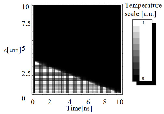
Figure 2.
Electron temperature density evolution in time and space in the case of one laser pulse of 100 fs irradiation of an Au surface for relaxation time.
The spatial-temporal distribution of the electrons’ thermal field produced by one laser pulse on an Au surface, when t = 100 fs and versus time (1 ps), is presented in Figure 3. It was obvious that the thermal field was constant and had a penetration depth in Au of about 2.5 µm. One may also observe from Figure 3 that in the first 200 fs, the electrons’ temperature increased linearly with time.

Figure 3.
Spatial-temporal distribution of the electrons’ thermal field generated by one laser pulse on an Au surface, when t = 100 fs and versus time (1 ps).
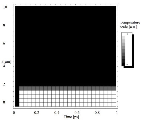
Figure 4.
Electron temperature density evolution in time and space in the case of one laser pulse of 100 fs irradiation of an Au surface for relaxation time vs. time (1 ps).
The same plot in Figure 1 is presented in Figure 5, but in this case for a Ag target (K = 429 W/mK, g = 2.3 × 10¹⁶ W/m3K). For silver, g/K is slightly smaller than for Au. The simulated electron temperature increased with about 0.3 a.u.
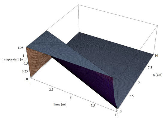
Figure 5.
Spatial-temporal distribution of electron temperature density in the case of one laser pulse of 100 fs irradiation of an Ag surface for relaxation time vs. time (10 ns).
In Figure 6, we plotted the same situation as in Figure 1, with the only difference that We observed a decrease in temperature close to 0.2 a.u.
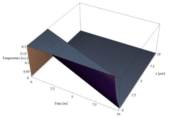
Figure 6.
Spatial-temporal distribution of electron temperature density evolution in the case of one laser pulse of 100 fs application onto an Au surface for relaxation time (10 ns).
When comparing Figure 1 and Figure 6, one can observe that the lower the relaxation time (0.5 ps vs. 1 ps), the lower the electron temperature (1200 K vs. 6000 K). In Figure 7, we plotted the spatial-temporal distribution of electron temperature density evolution (similar to Figure 6 with the only difference that the laser pulse was 20 fs). A drastic increment in temperature amplitude was observed for a very short time.
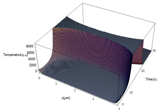
Figure 7.
Spatial-temporal distribution of electron temperature density evolution in the case of one laser pulse of 20 fs application onto an Au surface for relaxation time (10 ns).
Figure 8 shows the variation of the g/K value on temperature intensity and time when considering the following parameters: g = 1.05 × 10¹⁶ W/m3K, K = 315 W/mK, and laser pulse duration of 100 fs. The results demonstrate that as the g value is reduced down to one-half, the temperature intensity increased drastically, but preserved the shape of the 3D-heat field. A direct relationship was accordingly observed between relaxation time and temperature intensity. One important mention is that the temperature profile was identical to the 3D-heat field.
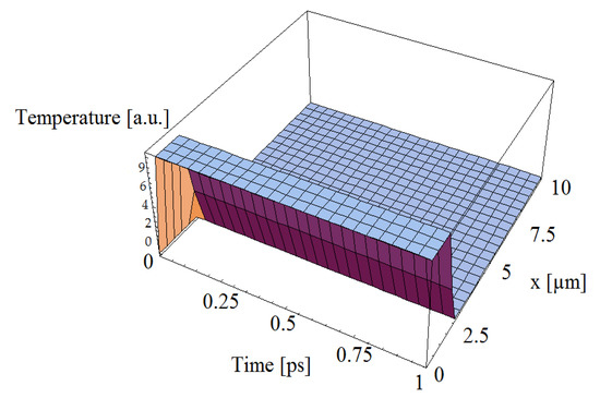
Figure 8.
The influence of g/K value on temperature intensity at g = 1.05 × 10¹⁶ W/m3K, K = 315 W/mK, and laser pulse duration of 100 fs.
4. Conclusions
The main conclusion of this study is that using state-of-the-art mathematics, TTM still can provide pertinent thermal information in ultra-short laser pulse–metal interaction [14]. This is due to the analytical description of the spatial-temporal behavior of a fs laser pulse interaction with matter, which is, in fact, the interaction of photons with atoms [15].
Some other conclusions are:
- (1)
- The computation time for the current model (using core i7 8th generation, 16.0 GB RAM) is equivalent to 1.5 min. This is much less than the numerical modeling of heat transfer in laser–metal interaction.
- (2)
- The lower the g/K factor, the higher the electron temperature. A lower g/K factor implies a reduced heat transfer from electrons to the lattice.
- (3)
- The lower the relaxation time, the lower the electron temperature. A lower relaxation time means a higher value of thermal speed () and a quick heat transfer between the electrons and the lattice.
- (4)
- Last, but not least, this model is based on the solution given by heat operators and therefore, is highly performing. On the other hand, it can be easily used by the researcher as the laser–metal interaction is treated in a classical way.
Author Contributions
Conceptualization, A.M.B., M.O., C.R., and B.A.S.; Methodology, M.O. and A.C.P.; Software, M.O. and M.A.M.; Validation, M.O., M.A.M., and A.C.P.; Writing—original draft preparation, A.M.B., M.O., and B.A.S.; Writing—review and editing, C.R. and I.N.M.; Supervision, C.R. and I.N.M. All authors have read and agreed to the published version of the manuscript.
Funding
This research was funded by the European Union’s Horizon 2020 (H2020) research and innovation program under the Marie Skłodowska-Curie (grant agreement no. 764935).
Acknowledgments
This work was supported by the Romanian Ministry of Education and Research under Romanian National Nucleu Program LAPLAS VI (contract 16N/2019). M.A.M. acknowledges the support from the European Union’s Horizon 2020 (H2020) research and innovation program under the Marie Skłodowska-Curie (grant agreement no. 764935). C.R. and I.N.M. acknowledge with thanks the partial financial support of this work under the contract POC-G 135/2016. A.C.P acknowledges financial support in the framework of Project PN-III-P1-1.1-TE-2016-2015 (TE136/2018). B.A.S acknowledges UEFISCDI, Executive Unit for Financing of Higher Education, Research and Innovation, Bucharest, Romania under projects PN-III-P1-1.2-PCCDI-2017-0871-contract 47PCCDI/2018 and PN-III-P1-1.2-PCCDI-2017-0619-contract 42PCCDI/2018.
Conflicts of Interest
The authors declare no conflicts of interest.
References
- Dyukin, R.V.; Martsinovskiy, G.A.; Sergaeva, O.N.; Shandybina, G.D.; Svirina, V.V.; Yakovlev, E.B. Interaction of femtosecond laser pulses with solids: Electron/phonon/plasmon dynamics. In Laser Pulses-Theory, Technology, and Applications; Peshko, I., Ed.; IntechOpen: Rijeka, Croatia, 2012. [Google Scholar]
- Shin, T.; Teitelbaum, S.; Wolfson, J.; Kandyla, M.; Nelson, K.A. Extended two-temperature model for ultrafast thermal response of band gap materials upon impulsive optical excitation. J. Chem. Phys. 2015, 143, 194705. [Google Scholar] [CrossRef] [PubMed]
- Jiang, L.; Tsai, H.-L. Improved two-temperature model and its application in ultrashort laser heating of metal films. J. Heat Trans. 2005, 127, 1167–1173. [Google Scholar] [CrossRef]
- Mihăilescu, I.N.; Oane, M.; Ticoş, C.M.; Ristoscu, C.; Bădiceanu, M. Linear Fourier Model Predictions in Case of Solids under IR FS Laser Irradiation. J. Las. Opt. Photonics 2019, 6, 194. [Google Scholar] [CrossRef]
- Anisimov, S.I.; Kapeliovich, B.L.; Perel’man, T.L. Electron emission from metal surfaces exposed to ultrashort laser pulses. Zh. Eksp. Teor. Fiz. 1974, 66, 776–781. [Google Scholar]
- Zhukovsky, K. Operational Approach and Solutions of Hyperbolic Heat Conduction Equations. Axioms 2016, 5, 28. [Google Scholar] [CrossRef]
- Zhukovsky, K. Operational solution for some types of second order differential equations and for relevant physical problems. J. Math. Anal. Appl. 2017, 446, 628–647. [Google Scholar] [CrossRef]
- Zhukovsky, K. Operational solution of differential equations with derivatives of non-integer order, Black-Scholes type and heat conduction. Mosc. Univ. Phys. Bull. 2016, 71, 237–244. [Google Scholar] [CrossRef]
- Zhukovsky, K.; Oskolkov, D.; Gubina, N. Some Exact Solutions to Non-Fourier Heat Equations with Substantial Derivative. Axioms 2018, 7, 48. [Google Scholar] [CrossRef]
- Prokhorov, A.M.; Konov, V.I.; Ursu, I.; Mihailescu, I.N. Laser Heating of Metals; Institute of Physics Publishing: London, UK, 1990. [Google Scholar]
- Lorin, E.; Chelkowski, S.; Bandrauk, A. A numerical Maxwell–Schrödinger model for intense laser–matter interaction and propagation. Comput. Phys. Commun. 2007, 177, 908–932. [Google Scholar] [CrossRef]
- Zhang, J.; Chen, Y.; Hu, M.; Chen, X. An improved three-dimensional two-temperature model for multi-pulse femtosecond laser ablation aluminum. J. Appl. Phys. 2015, 117, 063104. [Google Scholar] [CrossRef]
- Joseph, D.D.; Preziosi, L. Heat wave. Rev. Mod. Phys. 1989, 61, 41. [Google Scholar] [CrossRef]
- Oane, M.; Taca, M.; Tsao, S.L. Two Temperature Models for Metals: A New “Radical” Approach. Lasers Eng. (LIE) 2012, 24, 105–113. [Google Scholar]
- Li, S.L.; Huang, Z.P.; Ye, Y.K.; Wang, H.L. Femtosecond laser inscribed cladding waveguide lasers in Nd: LiYF4 crystals. Opt. Laser Technol. 2018, 102, 247–253. [Google Scholar] [CrossRef]


© 2020 by the authors. Licensee MDPI, Basel, Switzerland. This article is an open access article distributed under the terms and conditions of the Creative Commons Attribution (CC BY) license (http://creativecommons.org/licenses/by/4.0/).