Tribological Characterization of Ni-Free Duplex Stainless Steel Alloys Using the Taguchi Methodology

Abstract

Duplex stainless steels (DSSs) exhibit excellent corrosion resistance and are being used in a variety of industrial applications. Reducing/eliminating the amount of nickel in such alloys will contribute significantly to its economic viability. Moreover, a well-established wear behavior for these alloys is also an essential development in most of their applications. Hence, in this work, the Taguchi technique was effectively implemented to investigate the effect of operating factors such as sliding speed and applied load on the wear behavior of different compositions of nickel-free DSSs. It was observed that the composition had a higher contribution of 33.66% to the wear rate (WR) and the contribution of the sliding speed to the coefficient of friction (COF) was found to be 68.17%. With a good agreement, a regression model was also developed to predict the WR and COF within a certain range of factors. Wear tests have also shown that the developed nickel-free DSS is a promising candidate in terms of wear resistance as compared to austenitic stainless steels (ASS).

1. Introduction

Good tribological properties, resistivity to corrosion, a moderate strength, as well as good deformability make stainless steel (SS) alloys a preferential candidate to be used in different applications, such as structural [1,2], biomaterial [3], photocatalytic [4], nuclear [5], and biomedical [6,7,8,9]. Ferritic stainless steels (FSS) and austenitic stainless steels (ASS) are the two main types of SS alloys that are extensively used: 430 SS and 304 SS are examples of ferritic and austenitic stainless steels (ASS), respectively. Their chemical compositions are presented in

Table 1. Ferritic 430 and austenitic 304 alloys.

Structure	Grade	C	Si	Mn	P	S	N	Cr	Ni	Mo
Ferritic	430	0.08	1	1	0.04	0.015	-	16.0/18.0	-	-
Austenitic	304	0.07	1	2	0.045	0.015	0.11	17.5/19.5	8.0/10.5	-

. However, they still suffer from a few drawbacks in terms of their strength, resistance to stress corrosion cracking, the ability to be welded in thick sections, and their low toughness at low temperature [10].

Hence, to enhance the mechanical and corrosion properties of the SS alloys, duplex stainless steels (DSS) are being developed, which is a combination of ASS and FSS [11,12]. DSS exhibits a good combination of properties, such as good strength, toughness, corrosion resistance, and resistance to stress corrosion cracking, besides the economic benefits wherever it is needed. Muthupandi et al. [13] reported that controlling the composition as well as securing the proper balance of the microstructure (ferrite to austenite ratio) are the main factors to get the needed combination of good properties. Generally, the equal quantities of austenitic and ferritic phases along with the absence of precipitated phases guarantee good properties of the DSS alloys [14]. Producing the DSS needs to include the austenite stabilizers such as nickel (Ni), manganese (Mn), and nitrogen (N) in the composition of the DSS alloys. However, the higher price of Ni led to the need to reduce the amount of Ni in these alloys. Therefore, many studies have been reported to substitute Ni with other stabilizers to overcome the economic issues and securing the austenite stabilization along with the strength of the solid solution [15,16,17,18]. Moreover, not many studies have reported the wear behavior of these Ni-free DSS alloys. Hence, the main focus of this work is to investigate the effect of composition and other operating parameters, such as applied load and sliding speed, on the wear rate and the coefficient of friction (COF) of these Ni-free DSS alloys. Three Ni-free alloy samples with different compositions were used to run the tests under different operating factors. The optimized factors were used to study the comparison between the DSS alloys and ASS alloys. To effectively achieve these objectives, the Taguchi technique was used to design the experiments to come up with the optimum factors that shall lead to a low specific wear rate (SWR) and low COF.

2. Design of Experiments (DOE)

Among the most commonly used techniques for the design of experiments (DOE), such as the factorial and response surface method (RSM), the Taguchi technique is considered to be very effective since it offers a quality and simplicity to have an optimized design with an optimum cost [19]. The Taguchi technique is used to find out the best factors amongst the total operating factors by avoiding the full factorial experiment runs [20]. Recently, the Taguchi technique has evolved into an effective and popular statistical method in DOE in engineering applications [21,22,23,24] since it has the ability to configure an optimized design for the experiments by analyzing the effects of individual operating factors and also the influence of the interactions among them. Taguchi uses the orthogonal array (OA) and signal-to-noise ratio (S/N) as the two major tools to develop an optimized experimental design. Based on OA, the experiments are designed in such a way that the independent factors are arranged to be orthogonal to each other with securing all combinations of the operating factors. The S/N ratio analysis is used to measure the deviation of quality characteristic from the desired value by measuring the signal-to-noise ratio, which leads to finding out the optimum factors [25]. A higher S/N ratio is preferred in experimental designs, which reflects the minimum noise coming from uncontrollable sources during the tests. S/N ratio analysis has three different criteria to assess the design based on the need: “smaller is better”. nominal is better”, and “larger is better”. These criteria are given by the following equations:

Smaller is better:

$$\frac{S}{N}=-10 log\frac{1}{n}\left({\displaystyle \sum }_{i=1}^n{y}^2\right)$$

(1)

Nominal is better:

$$\frac{S}{N}=10 log\frac{y_{avg}}{S_y^2}$$

(2)

Larger is better:

$$\frac{S}{N}=-10 log\frac{1}{n}\left({\displaystyle \sum }_{i=1}^n\frac{1}{y^2}\right)$$

(3)

where y is the observed data, n number of observations, $y_{avg}$ is the average of the data observed, and $S_y^2$ is the variance. In this study, the main focus is to find out the optimum factors that would result in reducing the specific wear rate (SWR) and COF, and hence the “smaller-is-better” criteria was implemented in our investigation.

3. Experimental Procedures

3.1. Materials

A Schaeffer diagram was used to calculate the Ni equivalents to develop nickel-free DSS alloys with varying amounts of Mn and Cu, and their compositions are as shown in

Table 2. Compositions of the designed alloys.

Alloys	(x = 6, 5, 4, y = 0, 1, 2)
	Fe (Balance)	Cr 16	Mn x	Mo 1	Si 1	N 0.22	Cu y
DSS 1	Bal.	16	6	1	1	0.22	0
DSS 2	Bal.	16	5	1	1	0.22	1
DSS 3	Bal.	16	4	1	1	0.22	2

. The designed compositions confirmed that the alloys have a duplex microstructure [26,27]. The cast DSS alloys were prepared in-house in a vacuum arc melting (VAM) furnace, which were subsequently hot rolled to a thickness of 6 mm. The hot rolled alloys were then cold rolled (35%), and subsequently solution annealed followed by cold rolling again. In order to have an optimized phase balance (approximately 55% austenite + 45% ferrite), the alloys were solution annealed at 1070 °C, 1100 °C, and 1120 °C, respectively, based on Thermo-Calc calculations [28].

3.2. Roughness and Hardness Measurements

An optical profilometer (GTK-A, Bruker, USA) was used to conduct the roughness measurements on all the samples to make sure that all the samples have the same average surface roughness. A total of three to five measurements were carried out on each sample and the average value of roughness is reported. Hardness of the samples was measured by using a Rockwell Hardness testing machine (LECO Hardness tester R-600, United States of America). The applied load was 100 kgf for a time of 10 s with a spherical ball as an indenter.

3.3. Wear Test Procedure and the Taguchi Experimental Matrix

A ball-on-disc tribometer (UMT-3, Bruker, United States of America) was used to conduct the wear tests. The counter face used was a hardened stainless steel ball of grade 440C with a diameter of 6.3 mm and a hardness of RC 62. As mentioned earlier, the Taguchi technique was implemented to design our experiments and obtain the optimum factors that would affect the tribological performance of the designed alloys. Three main factors (Input parameters) were considered, namely, the composition of the alloys, the applied load and the sliding speed. Three levels for each of these factors were assigned as shown in

Table 3. Levels of the factors.

Factors	Level1	Level 2	Level 3
Composition	DSS 1	DSS 2	DSS 3
Speed (m/sec)	0.1	0.2	0.3
Load (N)	20	25	30

.

The L₉ orthogonal array (OA) Taguchi design was sufficient to represent the experiments with minimum number of runs wherein the optimization needs a total of nine runs with different combinations of factors and their respective levels. The nine runs of the OA are as shown in

Table 4. The runs of the orthogonal array (OA).

Runs	Composition	Speed (m/sec)	Load (N)
1	DSS 1	0.1	20
2	DSS 1	0.2	25
3	DSS 1	0.3	30
4	DSS 2	0.1	25
5	DSS 2	0.2	30
6	DSS 2	0.3	20
7	DSS 3	0.1	30
8	DSS 3	0.2	20
9	DSS 3	0.3	25

. All the tests were conducted at room temperature (25 ± 2 °C) and a relative humidity of 55% ± 5%. The test was repeated three times for each set of operating factors. As mentioned earlier, to achieve the objective of reducing the SWR and COF, the “smaller-is-better” criteria was implemented in our Taguchi design.

An optical microscope (MX7100, MEIJI, Hicksville, NY, USA) and a scanning electron microscope (SEM) (JSM-5800LV, JEOL, Japan) have been used for the analysis of the counterface ball and the wear track after the test to evaluate the wear of both the ball and the sample. An optical profilometer (GKT-A, Bruker, Billerica, MA, USA) was used to calculate the wear volume and subsequently the specific wear rate (SWR). The MINITAB software (MINITAB17, State College, PA, USA) was used to perform the S/N ratio and the ANOVA analysis. The regression model was developed after several iterations using MINITAB17 and MATLAB software (MATLAB2018a, Natick, MA, USA).

4. Results and Data Analysis

4.1. Hardness and Roughness Results

It can be clearly observed that all the Ni-free developed DSS alloys have a significantly higher hardness as compared to that of ASS as shown in

Table 5. Hardness test readings.

Alloys	Average Hardness (BHR)
DSS 1	88.2
DSS 2	87.94
DSS 3	86.02
ASS 304	75.54

. However, among the developed alloys, DSS1 showed a slightly higher hardness as compared to the other alloys. Roughness measurements were also conducted on all the samples after they were grounded and polished to obtain an average surface roughness of 0.014 ± 0.03 μm to make sure that the surface roughness does not contribute to the test results.

4.2. Effect of the Three Factors on Specific Wear Rate of the Developed DSS Samples

Before proceeding further, the analysis procedure for measuring the specific wear rate of the developed DSS samples with the aid of optical profilometry images is explained. Figure 1 shows the 3D, surface and 2D profiles of the wear track after the wear test measured using the optical profilometer. The wear test was conducted with the counterface ball sliding against the metallic sample in a circle with a 4 mm diameter (2r) for a sliding distance of 180 m. The specific wear volume was calculated using the following Equation (5):

SWR = (C × A)/(d × L)

(4)

$$SWR=\frac{C\ast A}{d\ast L}$$

(5)

where C is the circumference of the wear track (2πr), A is the cross-section area of the wear, d is the sliding distance, and L is the applied load. The cross section area of the wear track was calculated from the 2D profile of the wear track which, was obtained from the VISION 64 software of the optical profilometer.

Table 6. Specific wear rate results with the corresponding values of the signal-to-noise (S/N) ratios for the nine runs as specified by the OA of the Taguchi methodology.

Runs	Composition	Speed (m/sec)	Load (N)	Specific Wear Rate (mm3/Nm)				S/N Ratio (dB)
				Trial 1	Trial 2	Trial 3	Mean
1	DSS 1	0.1	20	0.000060	0.000060	0.000060	0.000060	84.44
2	DSS 1	0.2	25	0.000070	0.000080	0.000110	0.000087	81.08
3	DSS 1	0.3	30	0.000080	0.000080	0.000080	0.000080	81.94
4	DSS 2	0.1	25	0.000120	0.000120	0.000080	0.000107	79.31
5	DSS 2	0.2	30	0.000100	0.000090	0.000100	0.000097	80.28
6	DSS 2	0.3	20	0.000140	0.000130	0.000130	0.000133	77.50
7	DSS 3	0.1	30	0.000050	0.000080	0.000070	0.000067	83.37
8	DSS 3	0.2	20	0.000140	0.000130	0.000130	0.000133	77.50
9	DSS 3	0.3	25	0.000120	0.000100	0.000110	0.000110	79.15

shows the SWR and the S/N ratios for each of the nine runs/experiments as specified by the OA of the Taguchi methodology.

The main effects plots for the means and S/N ratios are shown in Figure 2 and Figure 3, respectively. Figure 2 shows the effect of the load on SWR. Increasing the load leads to a reduction in SWR, which can be attributed to the combined effect of the factors, such as the compositions and the sliding speed, which play a major role in affecting the wear rate; so, studying these changes are desired in such tests. By contrast, the sliding speed shows a direct proportion to the wear rate. The S/N ratio Figure 3 summarizes the effect of each factor by finding the average value for the S/N ratio related to that factor. Based on our criteria of “smaller-is-better”, composition DSS2, a sliding speed of 0.3 and a load of 20 N shows the lowest SWR, so these values are optimized factors for SWR within the selected range.

Using MINITAB17 software, ANOVA analysis was conducted with a 95% confidence level, which means that the level of significance (α) = 0.05. The latter is used to determine how much the factor is significant in the process. Generally, the principle of using ANOVA analysis is based on assuming a null hypothesis, which states that all the means are equal, and an alternative hypothesis that states that the means are unequal. Comparing the P-value with the level of significance (α) will support one of the hypotheses. The P-value in the ANOVA in

Table 7. ANOVA analysis for specific wear rate (SWR).

Source	DF	Seq SS	Contribution	Adj SS	Adj MS	F-Value	P-Value
Composition	2	0.00000	33.66%	0.00000	0.00000	15.49	0.0000
Speed	2	0.00000	25.71%	0.00000	0.00000	11.83	0.0000
Load	2	0.00000	18.89%	0.00000	0.00000	8.69	0.002
Error	20	0.00000	21.73%	0.00000	0.00000	-	-
Lack-of-Fit	2	0.00000	7.42%	0.00000	0.00000	4.67	0.0230
Pure Error	18	0.00000	14.31%	0.00000	0.00000	-	-
Total	26	0.00000	100.00%	-	-	-	-

shows that the factors are all significantly influencing the SWR because all the values are less than α. The magnitude of the P-value also helps in determining the most influential factors among all the factors used on the SWR, where a lower value indicates stronger evidence, which is clearly shown through the contribution values. It can be observed that the composition and sliding speed are more significant than the applied load on SWR.

4.3. Effect of the Three Factors on Coefficient of Friction of the Developed DSS Samples

Figure 4 shows a typical graph for COF vs. time for a wear test conducted on the DSS1 sample at a sliding speed of 0.3 m/s and at a load of 30N (Run #3 in

Table 8. Coefficient of friction results with the corresponding values of the S/N ratios for the nine runs as specified by the OA of the Taguchi methodology.

Runs	Composition	Speed (m/s)	Load (N)	COF				S/N Ratio (dB)
				Trial 1	Trial 2	Trial 3	Mean
1	DSS 1	0.1	20	0.6761	0.6658	0.6744	0.6721	3.45
2	DSS 1	0.2	25	0.5311	0.4579	0.4703	0.4864	6.24
3	DSS 1	0.3	30	0.3779	0.4218	0.4299	0.4099	7.73
4	DSS 2	0.1	25	0.5686	0.5473	0.5756	0.5638	4.98
5	DSS 2	0.2	30	0.3807	0.4104	0.4581	0.4164	7.58
6	DSS 2	0.3	20	0.4252	0.4386	0.4435	0.4358	7.21
7	DSS 3	0.1	30	0.4473	0.5760	0.5325	0.5186	5.66
8	DSS 3	0.2	20	0.4688	0.4738	0.4672	0.4699	6.56
9	DSS 3	0.3	25	0.4130	0.4145	0.3954	0.4076	7.79

). The reported COF is the average value for the steady-state region of the measurements. Table 8 shows the mean values and the corresponding S/N ratios of COF for each set of factors. Figure 5 and Figure 6 present the main effects plots for the means and S/N ratios, respectively.

On the evaluation of the individual effects of the three factors on the COF, it can be observed from Figure 5 that DSS1 shows a relatively high COF as compared to the other DSS alloys, which can be attributed to the higher hardness values of DSS1, which results in a greater resistance to shear, resulting in a higher COF. However, with an increase in the sliding speed and load a decrease in the COF is observed, which may be due to the surface softening because of the local rise in temperature that helps to reduce the shear strength which in turn reduces the COF. Figure 6 represents the plot of S/N ratios that takes into account the main and the interaction effects of the factors along with the criteria “smaller-is-better”. It can be seen from this plot that the optimum values of the three factors resulting in the lowest COF are for DSS1, at a sliding speed of 0.1 m/s and a load of 20 N.

Table 9. ANOVA analysis for COF.

Source	DF	Seq SS	Contribution	Adj SS	Adj MS	F-Value	P-Value
Composition	2	0.01776	8.83%	0.01776	0.00888	9.29	0.001
Speed	2	0.13710	68.17%	0.13710	0.06855	71.69	0.000
Load	2	0.02714	13.49%	0.02714	0.01357	14.19	0.000
Error	20	0.01912	9.51%	0.01912	0.00096	-	-
Lack-of-Fit	2	0.00194	0.97%	0.00194	0.00097	1.02	0.381
Pure Error	18	0.01718	8.54%	0.01718	0.00095	-	-
Total	26	0.20112	100.00%	-	-	-	-

shows the ANOVA analysis from which it can be deduced that all the factors contribute to the COF. However, the contribution of sliding speed to COF is found to be the highest with a contribution of 68.17% followed by that of load (13.49%) and then by composition (8.83%).

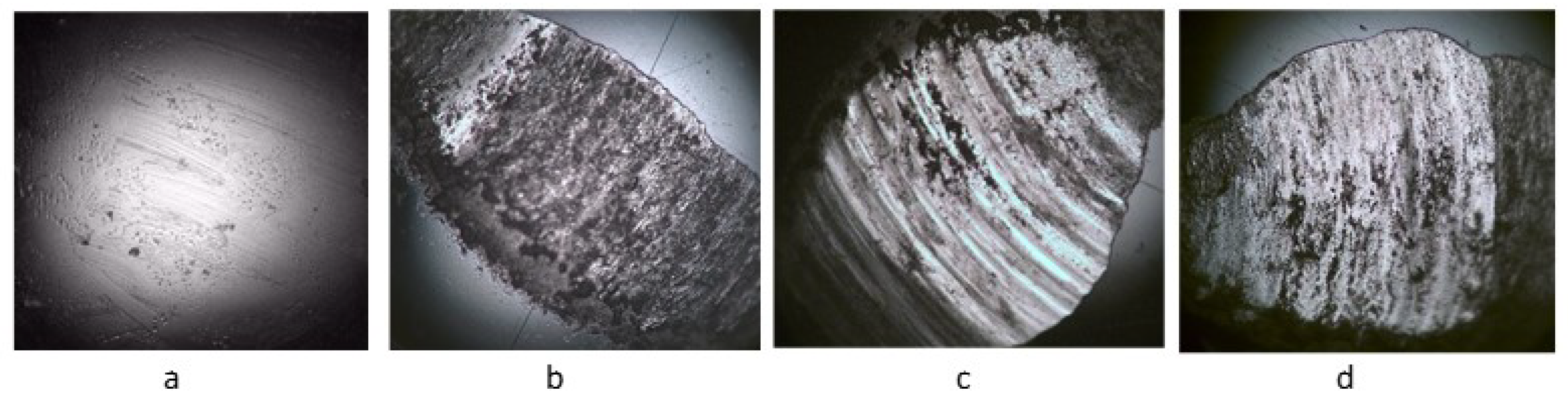
4.4. Evaluation of Involved Wear Mechanisms

The wear tracks and the counterface balls were analyzed after every wear test to evaluate the wear mechanisms involved. An optical microscope was used to evaluate the wear of the counterface ball and FESEM with EDS mapping was used to analyze the wear tracks. Figure 7 shows the typical optical images of the counterface ball images before and after the tribo tests. A big scar mark can be observed on the ball along with some debris particles attached. The scar can be attributed to the abrasive wear mechanism because of the ploughing effect by the asperities of the DSS sample. The debris particle transfer on to the ball can be indicative of an adhesive wear mechanism or the oxide film formation during the wear tests.

Figure 8, Figure 9 and Figure 10 show the SEM images of the wear tracks for the DSS1, DSS2 and DSS3 alloys after the wear tests at different magnifications. The images show clearly that the predominant mechanism is abrasive with deep grooves appearing on the wear track along the direction of motion. In addition to that, the appearance of debris on the wear track and on its side confirm the aforementioned explanation, which may be considered as a result of oxidation happening due to the dry sliding conditions confirmed by the EDS images in Figure 11, resulting in a three-body abrasion mechanism. Moreover, at few places on the wear track, deep tears were also observed, which are indicative of an adhesive wear mechanism. The reason behinds this is the mating of similar materials with the presence of high loads and a high sliding speed, leading to having some plastic deformation with the possibility to cause instantaneous welding that is broken, resulting in the tearing of the surfaces.

4.5. Regression Modeling

Based on the ANOVA analysis in the previous sections, it is observed that all the three operating factors (sliding speed, load and the composition) have a significance effect on both the SWR and the COF. Thus, a regression model should include all the factors to achieve a smooth fitting with the actual test results. Generally, the higher value of the R-square (R-sq) and a higher value of the adjusted R-square (R-sq(adj)), with a lower standard error estimate (S), indicate an acceptable fitting of the model with the experimental data. An individual regression model for each of SWR and COF has been developed with acceptable values of R-sq, R-sq(adj) and S as follows:

4.5.1. Regression Model for Specific Wear Rate (SWR)

Regression equation:

SWR = −0.000965275 + 0.0000100534 × C + 0.00650416 × S + 0.00000444747 × L − 0.00127778 × S² − 0.0000571946 × C × S − 0.0000338003 × S × L

(6)

Model summary:

S = 0.0375, R-sq = 84.7%, R-sq(adj) = 81.9%

(7)

4.5.2. Regression Model for COF

Regression equation:

COF = 666.187 − 15.3072 × C − 0.00752188 × L + 0.0880465 × C² + 4.42561 × S² − 0.0298231 × C × S

(8)

Model summary:

S = 0.0295, R-sq = 90.9%, R-sq(adj) = 88.8%

(9)

where, C is the composition of the sample and it takes the value of the hardness for each sample, such as for DSS1 “88.2”, DSS2 “87.94” and DSS3 “ 86.02”; S is the sliding speed levels (m/s); L is the applied normal load (N); SWR is the specific wear rate (mm³/N.m); and COF is the coefficient of friction.

The sign of the coefficient in the models’ equations shows the effect of each of the factors on the SWR and COF. For example, SWR is negatively correlated with composition with a coefficient of −0.000006, which means that increasing the hardness will reduce the SWR, which is reasonable and satisfy the formula $v=\frac{k.W.x}{H}$ However, the COF is positively correlated with composition where the coefficient has a value of +0.0

4.6. Model Confirmation

The confirmation of the developed regression model is essential to correlate the experimental results with the expected results. The confirmed model will indicate the validity of the approach of the Taguchi analysis. For this purpose, a set of factors with arbitrary values have been selected to run the experiments and then the model was used to estimate the values of SWR and COF. The difference and percent of error between the experimental results and model-predicted results were calculated and are as shown in

Table 10. Model confirmation for SWR and COF.

Sample	Comp.	Load (N)	Speed (m/s)	Specific Wear Rate (mm3/N.m)			COF
				Regression Model	Experiment	Error (%)	Regression Model	Experiment	Error (%)
1	DSS1	20	0.25	12.6421 × 10−5	13.2879 × 10−5	4.86	0.4954	0.5913	16.22
2	DSS1	25	0.3	10.1998 × 10−5	11.0936 × 10−5	8.06	0.4480	0.4734	5.38
3	DSS2	22.5	0.1	7.75073 × 10−5	9.06494 × 10−5	14.50	0.5872	0.4628	26.88
4	DSS2	30	0.15	9.25637 × 10−5	8.70125 × 10−5	6.38	0.4550	0.4918	7.48
5	DSS3	27.5	0.2	10.1667 × 10−5	12.4108 × 10−5	18.08	0.4136	0.4124	0.29
6	DSS3	20	0.3	14.595 × 10−5	13.5054 × 10−5	8.07	0.4347	0.3494	24.42

. It can be observed that the predicted values of SWR and COF using the developed regression model are in excellent agreement with the results of the actual experiment under the same conditions. It is worthy to mention that the model is helpful to determine the prediction values of the SWR and COF for such experiments in the range of this experiment’s factors.

5. Material Modification Effects

Once the optimum parameters for obtaining the lowest SWR and lowest COF were determined by the experimental runs of the OA designed by the Taguchi technique and the subsequent data analysis, we proceeded to check the performance of the DSS as compared to the ASS under those conditions.

Table 11. Optimum factors.

Optimum Operating Parameters	ASS		DSS1
	COF	SWR (mm3/N.m)	COF	SWR (mm3/N.m)
Low COF (Speed = 0.1m/s, Load = 20 N)	0.3414	0.000088	0.6707	0.00006
Low SWR (Speed = 0.3 m/s, Load = 20 N)	0.3072	0.000105	0.6721	0.00007

shows these factors with the corresponding SWR and COF values.

It can be observed that the SWR for the ASS sample is higher as compared to that of DSS1 under the same testing conditions, indicating the enhanced wear resistance of DSS1 alloys. However, the COF values for the ASS are lower than the DSS1 samples, which can be attributed to the lower hardness of the ASS alloys because of which the asperities at the contact surface are easily deformed plastically, resulting in lower shear stresses which in turn reduces the COF.

Table 12. Comparison of the results obtained in the present study with some of the existing studies in the literature.

Material Used	Speed (m/s)	Load (N)	SWR (mm3/N.m)	Ref.
Untreated AISI 316 austenitic stainless steel	0.2	5, 10, 20	0.00017–0.00020	[29]
Untreated AISI 304 austenitic stainless steel	0.044	up to 20	0.00009–0.000102	[30]
Super Duplex Stainless Steel AISI 2507	2, 4, 6	20, 40, 60	1.656–2.99	[31]
Duplex stainless steel	0.1, 0.2, 0.3	20, 25, 30	0.00006–0.00014	Current work

compares the results obtained in the present study in terms of the tribological properties with other SS alloys that have been studied under various conditions.

6. Conclusions

• The Taguchi technique was successfully implemented for designing the experiment, and the statistical results have offered a good reason to clarify and understand the effect of the operating factors on the tribological behavior of the DSS alloys.
• It was observed that all the three factors (composition, sliding speed and applied load) have a significant effect on SWR. However, it was observed that even though all three factors significantly affect the COF, the sliding velocity was found to be the most contributing factor to the COF behavior.
• The individual influence of the factors revealed that increasing the sliding speed decreases the SWR, and on the other hand, increasing the applied load increases SWR. For COF, the applied load shows the same behavior as SWR but opposite for the sliding speed. The COF increased with increasing the sliding speed, which was attributed to the increase in the localized temperature, which results in the softening of the metal leading to an increase in the contact area.
• It is also observed that the increase in the hardness of the DSS alloys improved their wear properties by reducing the SWR as compared to the ASS alloys. However, the DSS alloys showed a higher COF as compared to the ASS alloys, which is attributed to the high hardness of such materials compared to ASS.
• In conclusion, it can be stated that the DSS material is a promising candidate to be used in tribological applications due to their better wear resistance, corrosion resistance and high strength.

References

1. Baddoo, N.R. Stainless Steel in Construction: A Review of Research, Applications, Challenges and Opportunities. J. Constr. Steel Res. 2008, 64, 1199–1206. [Google Scholar] [CrossRef]
2. Dundu, M. Evolution of Stress–Strain Models of Stainless Steel in Structural Engineering Applications. Constr. Build. Mater. 2018, 165, 413–423. [Google Scholar] [CrossRef]
3. Pan, J.; Leygraf, C.; Thierry, D.; Ektessabi, A.M. Corrosion Resistance for Biomaterial Applications of TiO2 Films Deposited on Titanium and Stainless Steel by Ion-Beam-Assisted Sputtering. J. Biomed. Mater. Res. 1997, 35, 309–318. [Google Scholar] [CrossRef]
4. Jung, S.; Yong, K. Fabrication of CuO-ZnO Nanowires on a Stainless Steel Mesh for Highly Efficient Photocatalytic Applications. Chem. Commun. 2011, 47, 2643–2645. [Google Scholar] [CrossRef] [Green Version]
5. Segura, I.A.; Mireles, J.; Bermudez, D.; Terrazas, C.A.; Murr, L.E.; Li, K.; Injeti, V.S.Y.; Misra, R.D.K.; Wicker, R.B. Characterization and Mechanical Properties of Cladded Stainless Steel 316L with Nuclear Applications Fabricated Using Electron Beam Melting. J. Nucl. Mater. 2018, 507, 164–176. [Google Scholar] [CrossRef]
6. Dewidar, M.M.; Khalil, K.A.; Lim, J.K. Processing and Mechanical Properties of Porous 316L Stainless Steel for Biomedical Applications. Trans. Nonferrous Met. Soc. China 2007, 17, 468–473. [Google Scholar] [CrossRef]
7. Aggas, J.R.; Bhat, A.; Walther, B.K.; Guiseppi-Elie, A. Nano-Pt Ennobling of Stainless Steel for Biomedical Applications. Electrochim. Acta 2019, 301, 153–161. [Google Scholar] [CrossRef]
8. Bekmurzayeva, A.; Duncanson, W.J.; Azevedo, H.S.; Kanayeva, D. Surface Modification of Stainless Steel for Biomedical Applications: Revisiting a Century-Old Material. Mater. Sci. Eng. C 2018, 93, 1073–1089. [Google Scholar] [CrossRef]
9. Disegi, J.A.; Eschbach, L. Stainless Steel in Bone Surgery. Injury 2000, 31, D2–D6. [Google Scholar] [CrossRef]
10. Article: Duplex Stainless Steels—A Simplified Guide. Available online: https://www.bssa.org.uk/topics.php?article=668 (accessed on 17 April 2019).
11. Luo, H.; Su, H.; Dong, C.; Xiao, K.; Li, X. Electrochemical and Passivation Behavior Investigation of Ferritic Stainless Steel in Simulated Concrete Pore Media. Data Brief 2015, 5, 171–178. [Google Scholar] [CrossRef] [Green Version]
12. Lv, J.; Liang, T.; Wang, C.; Guo, T. Influence of Sensitization on Passive Films in AISI 2205 Duplex Stainless Steel. J. Alloy. Compd. 2016, 658, 657–662. [Google Scholar] [CrossRef]
13. Muthupandi, V.; Bala Srinivasan, P.; Seshadri, S.K.; Sundaresan, S. Effect of Weld Metal Chemistry and Heat Input on the Structure and Properties of Duplex Stainless Steel Welds. Mater. Sci. Eng. A 2003, 358, 9–16. [Google Scholar] [CrossRef]
14. Souza, E.C.; Rossitti, S.M.; Rollo, J.M.D.A. Influence of Chloride Ion Concentration and Temperature on the Electrochemical Properties of Passive Films Formed on a Superduplex Stainless Steel. Mater. Charact. 2010, 61, 240–244. [Google Scholar] [CrossRef]
15. Wang, J.; Uggowitzer, P.J.; Magdowski, R.; Speidel, M.O. Nickel-Free Duplex Stainless Steels. Scr. Mater. 1998, 40. [Google Scholar] [CrossRef]
16. Wessman, S.M.; Hertzman, S.; Pettersson, R.; Lagneborg, R.; Liljas, M. On the Effect of Nickel Substitution in Duplex Stainless Steel. Mater. Sci. Technol. 2008, 24, 348–355. [Google Scholar] [CrossRef]
17. Herrera, C.; Ponge, D.; Raabe, D. Design of a Novel Mn-Based 1GPa Duplex Stainless TRIP Steel with 60% Ductility by a Reduction of Austenite Stability. Acta Mater. 2011, 59, 4653–4664. [Google Scholar] [CrossRef]
18. Toor, I.-H.; Hyun, P.J.; Kwon, H.S. Development of High Mn–N Duplex Stainless Steel for Automobile Structural Components. Corros. Sci. 2008, 50, 404–410. [Google Scholar] [CrossRef]
19. Ribeiro, J.; Lopes, H.; Queijo, L.; Figueiredo, D. Optimization of Cutting Parameters to Minimize the Surface Roughness in the End Milling Process Using the Taguchi Method. Period. Polytech. Mech. Eng. 2017, 61, 30–35. [Google Scholar] [CrossRef]
20. Hong, Y.-Y.; Beltran, A.A.; Paglinawan, A.C. A Robust Design of Maximum Power Point Tracking Using Taguchi Method for Stand-Alone PV System. Appl. Energy 2018, 211, 50–63. [Google Scholar] [CrossRef]
21. Geethapriyan, T.; Muthuramalingam, T.; Vasanth, S.; Thavamani, J.; Srinivasan, V.H. Influence of Nanoparticles-Suspended Electrolyte on Machinability of Stainless Steel 430 Using Electrochemical Micro-Machining Process. In Advances in Manufacturing Processes 2019; Sekar, K.S.V., Gupta, M., Arockiarajan, A., Eds.; Springer: Singapore, Singapore, 2019; pp. 433–440. [Google Scholar]
22. Kar, A.; Balaji, G.; Tamang, S.; Aravindan, S. Mechanical Characterization of Gas Tungsten Arc Welded Super Duplex Stainless Steel Joint. Mater. Res. Innov. 2018, 22, 43–49. [Google Scholar] [CrossRef]
23. Dhananchezian, M.; Priyan, M.R.; Rajashekar, G.; Narayanan, S.S. Study the effect of cryogenic cooling on machinability characteristics during turning duplex stainless steel 2205. Mater. Today Proc. 2018, 5(Part 2), 12062–12070. [Google Scholar] [CrossRef]
24. Philip Selvaraj, D. Experimental Analysis of Surface Roughness of Duplex Stainless Steel in Milling Operation. In Advances in Manufacturing Processes 2019; Sekar, K.S.V., Gupta, M., Arockiarajan, A., Eds.; Springer: Singapore, Singapore, 2019; pp. 373–382. [Google Scholar]
25. Andrew Liou, Y.H.; Lin, P.P.; Lindeke, R.R.; Chiang, H.D. Tolerance Specification of Robot Kinematic Parameters Using an Experimental Design Technique—the Taguchi Method. Robot. Comput. Integr. Manuf. 1993, 10, 199–207. [Google Scholar] [CrossRef]
26. Prince, A.; Smolensky, P. Constraint Interaction in Generative Grammar; John Wiley & Sons: Hoboken, NJ, USA, 2004; p. 262. [Google Scholar]
27. Long, C.J. The Ferrite Content of Austenitic Stainless Steel Weld Metal. Weld. J. 1973, 52, 281s–297s. [Google Scholar]
28. Andersson, J.-O.; Helander, T.; Höglund, L.; Shi, P.; Sundman, B. Thermo-Calc & DICTRA, Computational Tools for Materials Science. Calphad 2002, 26, 273–312. [Google Scholar]
29. Sun, Y.; Bell, T. Dry Sliding Wear Resistance of Low Temperature Plasma Carburised Austenitic Stainless Steel. Wear 2002, 253, 689–693. [Google Scholar] [CrossRef]
30. Sun, Y. Sliding Wear Behaviour of Surface Mechanical Attrition Treated AISI 304 Stainless Steel. Tribol. Int. 2013, 57, 67–75. [Google Scholar] [CrossRef]
31. Davanageri, M.; Narendranath, S.; Kadoli, R. Dry Sliding Wear Behavior of Super Duplex Stainless Steel AISI 2507: A Statistical Approach. Arch. Foundry Eng. 2016, 16, 47–56. [Google Scholar] [CrossRef]
Figure 1. Representative images of the wear track from the optical profilometer for one of the experimental runs: (a) 3D profile; (b) surface profile; and (c) 2D profile.
Metals 10 00339 g001
Figure 2. Main effect plot for the mean specific wear rate.
Metals 10 00339 g002
Figure 3. Plot for the corresponding S/N ratios.
Metals 10 00339 g003
Figure 4. Typical graph for coefficient of friction (COF) vs. time for a wear test conducted on the DSS1 sample at a sliding speed of 0.3 m/s and at a load of 30N (Run #3 in Table 8).
Metals 10 00339 g004
Figure 5. Main effect plot for the mean COF.
Metals 10 00339 g005
Figure 6. Plot for the corresponding S/N ratios.
Metals 10 00339 g006
Figure 7. Microscopic images for the counterface ball (a) before and after for (b) DSS1, 0.2 m/s, 25 N; (c) DSS2, 0.1 m/s, 25 N; and (d) DSS3, 0.3 m/s, 25 N.
Metals 10 00339 g007
Figure 8. SEM images with different magnifications for the DSS1 tested sample with 0.1 m/s speed and 25 N load. (a) 60×, (b) 100× and (c) 500×.
Metals 10 00339 g008
Figure 9. SEM images with different magnifications for the DSS2 tested sample with 0.1 m/s speed and 25 N load. (a) 60×, (b) 100× and (c) 500×.
Metals 10 00339 g009
Figure 10. SEM images with different magnifications for the DSS3 tested sample with 0.3 m/s speed and 25 N load. (a) 60×, (b) 100× and (c) 500×.
Metals 10 00339 g010
Figure 11. SEM image of the wear track after the wear test along with the EDS mapping showing the presence of oxygen indicative of oxidative wear.
Metals 10 00339 g011