Abstract
In aluminum casting, the temperature of liquid aluminum and the dissolved hydrogen density are crucial factors to be controlled for the purpose of both quality control of molten metal and cost efficiency. However, the empirical and numerical approaches to predict these parameters are quite complex and time consuming, and it is necessary to develop an alternative method for rapid prediction with a small number of experiments. In this study, the machine learning models were developed to predict the temperature of liquid aluminum and the dissolved hydrogen content in liquid aluminum. The obtained experimental data was preprocessed to be used for constructing the machine learning models by the sliding time window method. The machine learning models of linear regression, regression tree, Gaussian process regression (GPR), Support vector machine (SVM), and ensembles of regression trees were compared to find the model with the highest performance to predict the target properties. For the prediction of the temperature of liquid aluminum and the dissolved hydrogen content in liquid aluminum, the linear regression and GPR models were selected with the high accuracy of prediction, respectively. In comparison to the numerical modeling, the machine learning modeling had better performance, and was more effective for predicting the target property even with the limited data set when the characteristics of the data were properly considered in data preprocessing.
1. Introduction
Quality control of molten metal is becoming increasingly crucial in the foundry industry as the rigorous demand for the specification is requested from the customers. The final quality of the casting products is greatly affected by the characteristics of the molten metal [1,2,3]. In order to control the casting defects of aluminum products, such as porosity and shrinkage cavity, it is particularly important to control the temperature of the liquid aluminum and the dissolved hydrogen content in the liquid aluminum during the melting process [4,5,6,7,8].
The temperature of the liquid aluminum can significantly affect the quality of the final product. If the pouring temperature is not sufficiently higher than the liquidus temperature, the fluidity of the liquid aluminum deteriorates and the defects such as blowholes or insufficient filling are likely to occur. If the temperature of the liquid aluminum is superheated over 800 °C, the oxidation reaction at the melt surface is promoted with the increase of the impurities or cracks. In addition, it is essential to control the temperature of the liquid aluminum efficiently in order to minimize the temperature loss [9,10]. The dissolved hydrogen content in the liquid aluminum should be also carefully controlled to meet the high-quality inspection [11,12,13]. Remarkably, hydrogen gas can be dissolved in the liquid state of aluminum, and the dissolved hydrogen in the molten aluminum remaining after the solidification will cause the defects such as pores or microporosity. Also, the dissolved hydrogen in excess of the solubility limit in liquid aluminum during solidification will come out of solution and diffuse into the bifilm gap. Finally, this bifilm defect can work as crack initiators and deteriorate the mechanical property of the casting products [14]. Therefore, it is important to control the temperature of liquid aluminum and the dissolved hydrogen content in the liquid aluminum during the melting process.
In earlier works, various models have been proposed to predict the temperature of the liquid aluminum based on the empirical [15,16] and numerical [17,18,19] approaches. Wang et al. examined the computational fluid dynamics(CFD)-Taguchi combined method for the design of process parameters to optimize the aluminum melting [16]. To understand the melting behavior of the liquid aluminum by each process parameter, Quintana et al. [17], Nieckele et al. [18], and Bulin’ ski et al. [19] proposed the numerical solutions considering the heat transfer and the flow behavior based on the process parameters. Numerous studies on the quantification of the dissolved hydrogen content in the liquid aluminum have also attracted much attention from researchers for a long time [11,20,21,22,23,24,25,26]. Various melt treatments to control the dissolved hydrogen content in the liquid aluminum such as gas bubbling filtration (GBF) [20,21], degassing agent [22,26], and ultrasonication [24,25,27] have been introduced. Among these techniques, the GBF is one of the most effective processes, which has an obvious effect on degassing of hydrogen in the liquid aluminum with minimizing the melt loss and the dross formation. Previous studies have reported on the effect of process parameters such as the GBF processing time, GBF rpm, and the type of impeller on the dissolved hydrogen content in the liquid aluminum [20,21,28,29].
Both the empirical and numerical approaches to evaluate the temperature of the liquid aluminum or the dissolved hydrogen content in the liquid aluminum can provide the understanding of the melt property or the flow behavior, but the limitations still exist: difficulty to establish the empirical model between the process parameters and the melt properties due to the non-linear relationship, and the limitation in the application of the derived model when new experimental data set is added or the boundary condition is changed.
Recently, the machine learning (ML) models have been used as an alternative way to overcome the limitations in the empirical and numerical models to successfully predict the material properties [30,31,32]. It has become increasingly popular with advantages of being able to quickly solve the problems compared to other models based on the empirical and numerical approaches, and has the strong ability to deal with discrete data. In some researches, the ML models have already been adapted for predicting the melt temperature [33,34] and the porosity [35,36] in various materials including the aluminum alloys. However, the ML model of the temperature of the liquid aluminum and the dissolved hydrogen content in the liquid aluminum based on the experimental data, with consideration of the combination of process parameters, has not been sufficiently proposed.
The present study focuses on developing the machine learning models for predicting the temperature of the liquid aluminum and the dissolved hydrogen content in the liquid aluminum based on the experimental data. The process parameters were selected based on the main factors that affect the target properties. Experiments were carried out under the various combinations of process parameters and experimental data were preprocessed to be used in the machine learning models. For the prediction of the temperature of the liquid aluminum and the dissolved hydrogen content in the liquid aluminum, five types of machine learning models (linear regression, regression tree, Gaussian process regression (GPR), Support vector machine (SVM), and ensembles of regression trees) were investigated with different options. The developed machine learning models have been compared using various statistical values through the new data set, and the performance of the developed machine learning model is also compared to that of the numerical model.
2. Materials and Methods
The material used in the present study was pure aluminum ingot (>99.7 wt.%), and aluminum molten metal was produced in a high-frequency melting furnace. The main process parameters affecting the melt temperature and the dissolved hydrogen content in the liquid aluminum were selected, and the parameter studies were conducted under the various combination of experimental conditions to construct the data set for developing of the machine learning models as listed in Table 1. The temperature of the liquid aluminum was measured by k-type thermocouples. The applied electric power use during melting process was monitored using a real-time energy monitoring system (BMT Co., Ltd., Yangsan, South Korea). In the GBF process, the argon gas was selected as an inert gas. The dissolved hydrogen content in the liquid aluminum was measured by HYCAL (EMC Hycal Limited, Stafford, UK), which is a real time analyzer.

Table 1.
Process parameters to construct machine learning models for the temperature of the liquid aluminum and the dissolved hydrogen content in the liquid aluminum.
3. Machine Learning Modeling
3.1. Data Acquisition
The temperature of liquid aluminum during the melting process is strongly influenced by the input electric power condition, the weight of ingot, and the initial temperature of the liquid aluminum. At different power conditions of 15, 20, 25, and 30 kW, the temperature of the liquid aluminum was measured during the application time of electric power in the form of the time series data. The temperature of the liquid aluminum was also measured for different ingot weights of 4, 6, and 7 kg. The dissolved hydrogen content in the liquid aluminum is closely related to the process parameters of the GBF treatment condition, the temperature of liquid aluminum, and the initial hydrogen concentration. Under the fixed GBF rpm of 1510, a gas flow rate of 2, 4, 6, and 7 cc/min was set as variables. The temperature of liquid aluminum was also considered as a variable with 700, 730, 740, 760, 770, 790, and 800 °C being the selected temperatures. The dissolved hydrogen content was also measured during GBF treatment time in the form of the time series data. Figure 1 demonstrates one example of the data set to be used for developing machine learning model to predict the temperature of the liquid aluminum and the dissolved hydrogen content in the liquid aluminum.
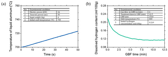
Figure 1.
One data set example for (a) temperature of liquid aluminum and (b) dissolved hydrogen concentration. GBF means gas bubbling filtration.
3.2. Data Acquisition
In this work, the machine learning approach involved the data generation process. The generated data comes from the original data set measured by the experiments according to the sliding time window method, which is regularization technique known to improve model performance [37,38,39]. Here, the sliding time window method was implemented in both the temperature of the liquid aluminum and the dissolved hydrogen content in the liquid aluminum.
For the temperature of the liquid aluminum, a window size (, = 1–9) was chosen as 5, 10, 15, 20, 25, 30, 40, 50, and 60 s. The input () and output () data set for training, validating, and testing were composed as follows: {Electric power, Ingot weight, , } and {} ( = 1,2,3,…), where represents the data of start point of the temperature of the liquid aluminum before sliding the window, represents the temperature of the liquid aluminum after sliding the window of , means the step size which is a constant of 3. From the sliding time window method, the number of the training, validating, and testing data set of the temperature of the liquid aluminum was prepared as 6067.
In the case of the dissolved hydrogen content in the liquid aluminum, a window size (, = 1–10) was chosen as 0.5, 1, 1.5, 2, 2.5, 3, 5, 7.5, 10, and 12.5 min. The input () and output () data set for training, validating, and testing were composed as follows: {Gas flow rate, GBF rpm, Melt temperature, , } and {} ( = 1, 2, 3, …), where represents the data of start point of the dissolved hydrogen content before sliding the window, represents the dissolved hydrogen content after sliding the window of , means the step size which is a constant of 1. After conducting the sliding time window method, the number of training, validating, and testing data set of the dissolved hydrogen content in the liquid aluminum was prepared as 5974. Note that this data generation process increases the amount of input data set in number, and it is originated from the original experimental data, not an artificial or imaginary data.
3.3. Machine Learning Model
The prepared data set was imported into MATLAB as an excel file format. The statistics and machine learning toolbox was used in this work, which provides the functions and apps to describe, analyze, and model data [40,41]. The toolbox provides the supervised machine learning algorithms such as support vector machine, boosted and bagged decision tree, k-nearest neighbor, and Gaussian mixture models etc.
In this work, the machine learning models of linear regression models, regression trees, Gaussian process regression models, support vector machines, and ensembles of regression trees were investigated to predict the temperature of the liquid aluminum and the dissolved hydrogen content in the liquid aluminum.
In general, the linear regression model can be described by the form
where is the ith response; is the kth coefficient ( is the constant term in the model); is the ith observation on the jth predictor variables (j ); is the ith noise term for random error and is a scalar-valued function of the independent variables (), which might be in any form including nonlinear functions or polynomials [42,43,44]. We used four different types of linear regression models (linear, interaction linear, robust linear, and stepwise linear) to confirm which setting produces the best result with the data. We chose the linear term for linear and robust linear models and the interactions term for interaction linear model. For the stepwise linear model, we set the linear, interactions and 1000 for initial terms, upper bound on terms and maximum number of steps, respectively.
The regression trees are one of the nonparametric supervised learning algorithms with low on memory usage and the standard Classification And Regression Tree (CART) algorithm is used by default. [44,45] In order to avoid overfitting, the smaller trees with fewer larger leaves can be tried first and then the larger trees are considered. We tested three different types of regression tree model (fine tree, medium tree, and coarse tree) with different minimum leaf sizes. In general, a fine tree with small leaves shows higher accuracy on the training data but it might not show comparable accuracy on an independent test set. In contrast, a coarse tree with large leaves does not give high accuracy for the training data but its training accuracy can be applied to a representative test set of data [41]. The regression trees which we used in this work were binary and each step in a prediction involved checking the value of one predictor variable. The minimum leaf size was 4, 12, and 36 for fine, medium, and coarse trees, respectively.
The Gaussian process regression (GPR) models are nonparametric kernel-based probabilistic models which explain the response by introducing latent variables, , from a Gaussian process (GP) and explicit basis functions. A Gaussian process is a set of random variables, having a joint Gaussian distribution, and is defined by its mean function and covariance function, . When , that is are from a zero mean GP with covariance function, , the joint distribution of latent variables in the GPR model can be described as follows in vector form:
where . The covariance function can be defined by various kernel functions, which can be parameterized in terms of the kernel parameters in vector , thus the covariance function can be expressed as [46,47]. In this work, we performed the prediction by using four different kernel functions such as rational quadratic, exponential, squared exponential, and matern 5/2 kernels. The detailed kernel functions are listed in Table 2.
Table 2.
Kernel functions for Gaussian process regression.
The support vector machine (SVM) regression is another nonparametric technique. The SVM finds the support vectors having a maximum margin after classifying the collected data into clusters by using a hyperplane [48]. The best hyperplane is the one with the largest margin between the classes. The linear -insensitive loss function, , is determined based on the distance between observed value and the margin . The error within the margin () of the observed value is ignored by treating them as zero as described below [41,49].
The SVM regression also relies on kernel functions and three different kernel functions such as linear, Gaussian, and polynomial were considered in this work. The details of the kernel functions are listed in Table 3. We performed the prediction with several models with linear, quadratic, cubic, fine Gaussian, medium Gaussian, and coarse Gaussian SVM to see the performance of each model. The kernel scales were set to , , for fine, medium, and coarse Gaussian SVM models, respectively, where is the number of predictors.
Table 3.
Kernel functions for Gaussian process regression.
The ensembles of regression trees are multi-learning algorithm techniques that complement the individual machine learning algorithms, and the bagged tree and boosted tree are typical [50,51]. The bagged tree makes a decision by constructing the tree by training the variables that are composed by randomly extracting the same size from the independent variables, and the boosted tree reinforces the learning as a whole by adjusting the weight of the weak learning [46,52]. In this work, the minimum leaf size and number of learners were set to 8 and 30 for both methods, and the learning rate of 0.1 was used for the boosted tree model.
The architectures of the machine learning model to predict the temperature of the liquid aluminum and the dissolved hydrogen content in the liquid aluminum are shown in Figure 2. To build models for predicting the final temperature of the liquid aluminum after applying the electric power and the final dissolved hydrogen content after the GBF treatment, 5922 and 5773 sets of data were used as the training/validation data set, respectively. The five-fold cross-validation scheme was used to protect against overfitting for model trainings. We compared the models with different options in each model type and selected the models with the best performance for each model type, which are shown in Figure 3 and Figure 6. The selected models were finally compared by using the new data set.
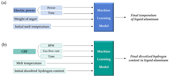
Figure 2.
The architectures of the machine learning model to predict the (a) temperature in liquid aluminum and (b) dissolved hydrogen content in liquid aluminum.
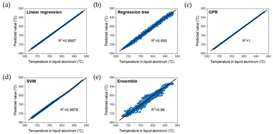
Figure 3.
Scatter plots of predicted values versus experimental values of temperature of liquid aluminum for different machine learning (ML) models of (a) linear regression, (b) regression tree, (c) Gaussian process regression (GPR), (d) support vector machine (SVM), and (e) ensemble regression trees.
4. Results and Discussion
4.1. Melt Temperature of the Liquid Aluminum
Figure 3 shows the scatter plots of the predicted values versus the experimental data of the temperature for the liquid aluminum with the machine learning models with the highest accuracy in each model type. The performance of the models seems to be similar as the coefficients of determination were close to 1 for all models; this means that the given data set of the temperature of the liquid aluminum was linear in nature.
The statistical comparison between the original experiments and the predicted values by five different machine learning models revealed that most of characteristics of the original data were captured by the developed models. For example, the mean, median, minimum, maximum, and standard deviation from experimental data were 744.5, 743.1, 704,9, 787.1, and 19.2, respectively, and those for the predicted values by linear regression model were 744.9, 743.2, 705.6, 787.5, and 19.5, respectively. The statistics comparisons of other models are listed in Table 4. In Table 5, the evaluation of the performance of the five different regression models developed in this work are compared. The root mean square error for GPR model was the smallest and followed by the linear regression model. Since the original data and the predicted values had a strong linear correlation for the melt temperature of the liquid aluminum data set, the linear regression model can be a proper model to predict if the accuracy is sufficient, which is known as one of the simplest machine learning models [53,54].
Table 4.
Comparison between the statistics of the predicted values using different machine learning models with that of the experimental data of the temperature of the liquid aluminum.
Table 5.
Evaluation of the performance of five regression models used to predict the value of the temperature of the liquid aluminum.
Figure 4 shows the probability distribution function (PDF) and cumulative distribution function (CDF) plots of new experiments and the prediction of the temperature of the liquid aluminum by the developed models. The PDF curves were fitted using the normal distribution option. The new experimental data in Figure 4 were obtained with 6 kg of aluminum ingot and 27 kW of electric power conditions under various times for electric power with 145 sets of data, which were not used for the development of machine learning model. The estimated parameters of the experimental data set from the normal distribution are listed in Table 6. In Figure 5, the comparison of measured values by experiments versus predicted values by linear regression model is shown with good agreement between the measurement and the predicted values with R2 of 0.9994.
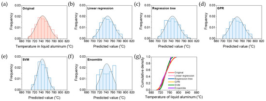
Figure 4.
Data distribution of temperature of liquid aluminum from (a) new experiment for prediction and predicted value by different machine learning (ML) models of (b) linear regression, (c) regression tree, (d) GPR, (e) SVM and (f) ensemble regression trees. The colored area in each graph of (a–f) (red, or blue) describes corresponding probability density function for the data distribution. (g) The corresponding cumulative density function for predicted values from each ML model compared to the histogram of the experimental value of temperature of liquid aluminum.
Table 6.
The estimated parameters from the normal distribution. μ is the mean of the melt temperature and is the square root of the unbiased estimator of the variance.
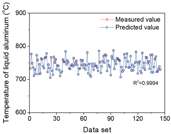
Figure 5.
The comparison between measured values by experiment versus predicted values by linear regression model for temperature of liquid aluminum.
4.2. Dissolved Hydrogen Content in the Liquid Aluminum
The sets of scatter plots between the predicted values from the machine learning models with the highest accuracy in each model type and the experimental data of the dissolved hydrogen content in the liquid aluminum are shown in Figure 6.
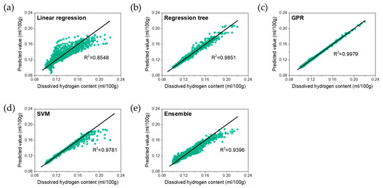
Figure 6.
Scatter plots of predicted values versus experimental values of dissolved hydrogen content in liquid aluminum for different ML models of (a) linear regression, (b) regression tree, (c) GPR, (d) SVM, and (e) ensemble regression trees.
The statistical comparisons between the original experiments and the predicted values by five different machine learning models are presented in Table 7 and show that the predictions from the GPR model are in the best agreement with the experimental data. The mean, median, minimum, maximum, and standard deviation from experimental data are 0.1194, 0.115, 0.1, 0.22, and 0.0143, respectively, and those for the predicted values by the GPR model are 0.1194, 0.1149, 0.0999, 0.2175, and 0.0142, respectively. The coefficients of determination are over 0.93 except the linear regression model with the value of 0.8548, as shown in Table 8.
Table 7.
Comparison between the statistics of predicted values using different machine learning models with that of the experimental data of the hydrogen content in the liquid aluminum.
Table 8.
Evaluation of the performance of five regression models used to predict the value of the dissolved hydrogen content in the liquid aluminum.
Figure 7 shows the probability distribution function (PDF) and the cumulative distribution function (CDF) plots of new experiments and the prediction of the dissolved hydrogen content in the liquid aluminum by the developed models. The PDF curves were fitted by using the lognormal distribution option, and the estimated parameters of the experimental data set from the normal distribution are listed in Table 9. The new experimental data in Figure 7 were obtained with 740 °C of the temperature of the liquid aluminum and 6 cc/min of gas flow rate conditions under various treatment times in GBF with 201 sets of data, which were not used for the development of machine learning model. The PDF plot for the predicted values by the GPR model closely follow the actual measurements over a wide range of the hydrogen content, showing the left-shift shape of the fitting curve and covering high content region over 0.14 mL/100 g. The CDF in Figure 7g also shows that the curve by GPR model closely captured the original data curve, indicating that the GPR model was the most accurate model to predict the dissolved hydrogen content in the liquid aluminum compared to the other models considered in this work. Figure 8 shows the comparison of measured values versus the predicted values by the GPR model with good agreement each other overall range of data set.
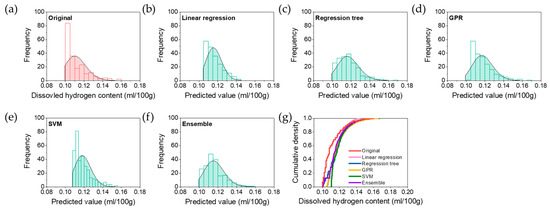
Figure 7.
Data distribution of dissolved hydrogen content in liquid aluminum temperature from (a) experimental results and predicted value by different ML models of (b) linear regression, (c) regression tree, (d) GPR, (e) SVM, and (f) ensemble regression trees. The colored area in each graph of (a–f) (red, or green) describes corresponding probability density function for the data distribution. (g) The corresponding cumulative density function for predicted values from each ML model compared to the histogram of the experimental values of the dissolved hydrogen content in liquid aluminum.
Table 9.
The estimated parameters from the lognormal distribution. μ is the mean of logarithmic values of the dissolved hydrogen content in liquid aluminum and σ is the standard deviation of logarithmic values.
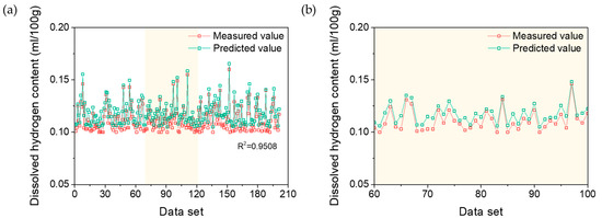
Figure 8.
(a) The comparison of measured values by experiment versus predicted values by GPR model for dissolved hydrogen content in the liquid aluminum, and (b) the magnified graph in the selected range.
4.3. Comparison of ML Model to Numerical Model
Based on the experimental results, a numerical model to predict final target properties of the temperature of the liquid aluminum and the dissolved hydrogen content in the liquid aluminum was investigated. Here, the numerical model was proposed using the raw data form without the data generation process used in constructing the machine learning model.
The temperature of the liquid aluminum had a linear relationship with the application time of electric power as shown in Figure 1a. The linear function was a form of , where is the slope and is the intercept of . The slope () and intercept () of linear relationship between the temperature of the liquid aluminum () and the application time of the electric power () depend on the experimental conditions. The slope and intercept are identified under all the experimental conditions, and one example is shown in Figure 9a under the electric power of 25 kW with the ingot weight of 4 kg. In particular, the most influential factors affecting the slope of this linear relationship were found to be the electric power and the ingot weight. Generally, the larger the weight of ingot, the higher level of electric power was required for melting of ingot. Therefore, the values of slope were plotted as a function of electric power/ingot weight (z, kW/kg) as shown in Figure 9b, and it was also fitted with the linear function: . The intercept values () of linear relationship between the temperature of the liquid aluminum and the application time of electric power show fairly similar values of 697.014 to 701.921, therefore is assumed to be 700.141 from the average of the obtained intercept values. Finally, the numerical model to predict the temperature of liquid aluminum is suggested as: , where is the electric power/ingot weight. Using the test data set described in Figure 5, the temperature of the liquid aluminum was predicted based on the suggested numerical model, as shown in Figure 9. By comparing with the results predicted by the linear regression model from the ML approach, the numerical model showed a comparable performance of R2 of 0.9961 with a simple assumption and approach, but the performance of numerical model was still lower than that of ML model.
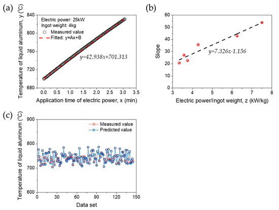
Figure 9.
(a) Linear fitting of measured value (one example of experimental results: electric power 25 kW, ingot weight 4 kg), and (b) numerical approach via electric power/ingot weight. (c) The comparison of measured value by experiment versus predicted values by empirical model of melt temperature for validation.
The dissolved hydrogen content in the liquid aluminum has the characteristics in which it converges over time as shown in Figure 1b. For this data type, it can be fitted well with a function of , where is the dissolved hydrogen content, is the GBF time, , , and are the fitted parameters. Using all of the experimental data sets, the fitted parameters were obtained, and one example of a fitting result is described in Figure 10a. The temperature of the liquid aluminum and the gas flow rate are considered to the most influential factors affecting final dissolved hydrogen content. Therefore, , , and are plotted as functions of melt temperature and gas flow rate as shown in Figure 10b–d. In this case, it is hard to find the numerical relationship between the fitted parameters of , , and experimental condition at this state due to the limited number of data set and simple assumption. In addition, the parameter of the dissolved hydrogen content is complicatedly influenced by the experimental conditions compared to the temperature of the liquid aluminum, which shows relatively simple linear relationship depending on the experimental parameters. Therefore, it can be said that the machine learning model is more effective in predicting the data set with a non-linear type. Also, the prediction model using the machine learning approach can be obtained with the high level of performance through the data generation process considering the data characteristic, even in hard case of constructing the numerical model.
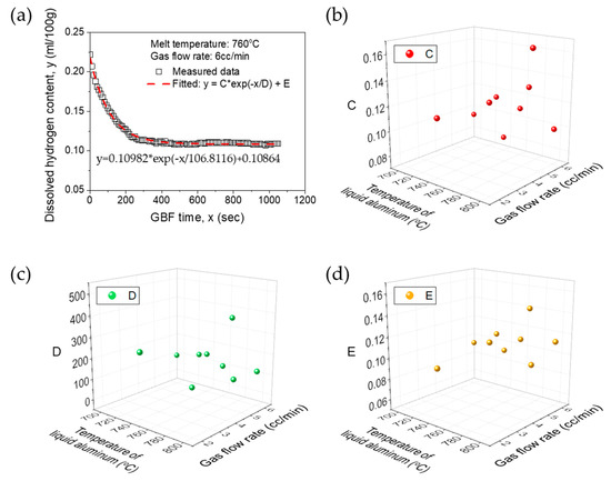
Figure 10.
(a) Numerical fitting of measured value (one example of experimental results: temperature of liquid aluminum 760 °C, gas flow rate 6 cc/min). Fitted parameters of (b) C, (c) D, and (d) E depending on temperature of liquid aluminum and gas flow rate.
5. Conclusions
In this study, the temperature of the liquid aluminum and the dissolved hydrogen content in the liquid aluminum were predicted with a machine learning approach. The temperature of the liquid aluminum and the dissolved hydrogen content in the liquid aluminum were the time series data set, so the limited number of the experimental data was preprocessed to be used to develop the machine learning models based on sliding time window method. Five types of machine learning models, including linear regression, regression tree, GPR, SVM, and ensembles of regression trees, were constructed for predicting the target properties. In order to confirm model performance, the constructed machine learning models based on training/validation data set were tested with new experimental data sets. In the case of the temperature of the liquid aluminum, five kinds of machine learning models showed the comparable model performance, and the linear regression can be used with high accuracy. To predict the dissolved hydrogen content, the GPR model showed the highest level of accuracy of prediction. For comparison, the numerical model was also investigated. The temperature of liquid aluminum had linear relationship between the experimental parameters of electric power and ingot weight, and it can be predicted by simple numerical approach using the linear function. However, the performance of the numerical model to predict temperature of the liquid aluminum was still lower than that of developed machine learning model of linear regression. The numerical model to predict the dissolved hydrogen content can be hardly obtained due to the limited data set and the highly non-linear characteristic of data set between the dissolved hydrogen content and the GBF process conditions. In order to apply prediction of melt property with a machine learning approach in real industry, more data acquisition considering various processing parameters will be still required. Nevertheless, from this work, it can be suggested that the machine learning model can be effective for predicting the target properties with high accuracy, even with the limited data set, when the data preprocessing takes into account the characteristics of the data properly.
Author Contributions
Conceptualization, validation, formal analysis, writing and editing, M.-J.K.; methodology, validation and review, J.P.Y.; data curation and investigation, J.-B.-R.Y. and S.-J.C.; Conceptualization, validation, writing, review and supervision, D.K. All authors have read and agreed to the published version of the manuscript.
Funding
This research was supported by the National Research Foundation of Korea (NRF) grant funded by the Korea government (MSIT) (No. 2017R1C1B2012459) and the Korea Institute of Industrial Technology as “KITECH’s Manufacturing Innovation Project (No. KITECH JH-19-0001).
Conflicts of Interest
The authors declare no conflict of interest.
References
- Puga, H.; Barbosa, J.; Gabriel, J.; Seabra, E.; Ribeiro, S.; Prokic, M. Evaluation of ultrasonic aluminium degassing by piezoelectric sensor. J. Mater. Process. Technol. 2011, 211, 1026–1033. [Google Scholar] [CrossRef]
- Dong, X.; Yang, H.; Zhu, X.; Ji, S. High strength and ductility aluminium alloy processed by high pressure die casting. J. Alloys Compd. 2019, 773, 86–96. [Google Scholar] [CrossRef]
- Bejaxhin, A.B.H.; Paulraj, G.; Prabhakar, M. Inspection of casting defects and grain boundary strengthening on stressed Al6061 specimen by NDT method and SEM micrographs. J. Mater. Res. Technol. 2019, 8, 2674–2684. [Google Scholar] [CrossRef]
- Fritzsche, A.; Hilgenberg, K.; Teichmann, F.; Pries, H.; Dilger, K.; Rethmeier, M. Improved degassing in laser beam welding of aluminum die casting by an electromagnetic field. J. Mater. Process. Technol. 2018, 253, 51–56. [Google Scholar] [CrossRef]
- Xu, H.; Han, Q.; Meek, T.T. Effects of ultrasonic vibration on degassing of aluminum alloys. Mater. Sci. Eng. A 2008, 473, 96–104. [Google Scholar] [CrossRef]
- Xiong, B.; Lin, X.; Wang, Z.; Yan, Q.; Yu, H. Microstructures and mechanical properties of vacuum counter-pressure casting A357 alloys solidified under grade-pressurising: Effects of melt temperature. Mater. Sci. Eng. A 2014, 611, 9–14. [Google Scholar] [CrossRef]
- Wang, F.; Wang, N.; Yu, F.; Wang, X.; Cui, J. Study on micro-structure, solid solubility and tensile properties of 5A90 Al–Li alloy cast by low-frequency electromagnetic casting processing. J. Alloys Compd. 2020, 820, 153318. [Google Scholar] [CrossRef]
- Liu, Y.; Jie, W.; Gao, Z.; Zheng, Y. Investigation on the formation of microporosity in aluminum alloys. J. Alloys Compd. 2015, 629, 221–229. [Google Scholar] [CrossRef]
- Yolshina, L.A.; Kvashinchev, A.G. Chemical interaction of liquid aluminum with metal oxides in molten salts. Mater. Des. 2016, 105, 124–132. [Google Scholar] [CrossRef]
- Monroe, R. Porosity in Castings. AFS Transcations 2005, 5, 1–28. [Google Scholar] [CrossRef]
- Mitrasinovic, A.; Robles Hernández, F.C.; Djurdjevic, M.; Sokolowski, J.H. On-line prediction of the melt hydrogen and casting porosity level in 319 aluminum alloy using thermal analysis. Mater. Sci. Eng. A 2006, 428, 41–46. [Google Scholar] [CrossRef]
- Zhao, L.; Pan, Y.; Liao, H.; Wang, Q. Degassing of aluminum alloys during re-melting. Mater. Lett. 2012, 66, 328–331. [Google Scholar] [CrossRef]
- Lapham, D.P.; Schwandt, C.; Hills, M.P.; Kumar, R.V.; Fray, D.J. The detection of hydrogen in molten aluminium. Ionics (Kiel) 2002, 8, 391–401. [Google Scholar] [CrossRef]
- El-Sayed, M.A.; Hassanin, H.; Essa, K. Bifilm defects and porosity in Al cast alloys. Int. J. Adv. Manuf. Technol. 2016, 86, 1173–1179. [Google Scholar] [CrossRef]
- Kumar, S.; Gupta, A.K.; Chandna, P. Optimization of Process Parameters of Pressure Die Casting using Taguchi Methodology. World Acad. Sci. Eng. Technol. 2012, 6, 590–594. [Google Scholar]
- Wang, J.-M.; Yan, H.-J.; Zhou, J.-M.; Li, S.-X.; Gui, G.-C. Optimization of parameters for an aluminum melting furnace using the Taguchi approach. Appl. Therm. Eng. 2012, 33, 33–43. [Google Scholar] [CrossRef]
- Quintana, I.; Azpilgain, Z.; Pardo, D.; Hurtado, I. Numerical Modeling of Cold Crucible Induction Melting. In Proceedings of the 2011 COMSOL conference, Stuttgart, Germany, 26–28 October 2011. [Google Scholar]
- Nieckele, A.O.; Naccache, M.F.; Gomes, M.S.P. Numerical Modeling of an Industrial Aluminum Melting Furnace. J. Energy Resour. Technol. 2004, 126, 72–81. [Google Scholar] [CrossRef]
- Buliński, P.; Smolka, J.; Golak, S.; Przyłucki, R.; Palacz, M.; Siwiec, G.; Melka, B.; Blacha, L. Numerical modelling of multiphase flow and heat transfer within an induction skull melting furnace. Int. J. Heat Mass Transf. 2018, 126, 980–992. [Google Scholar] [CrossRef]
- Brůna, M.; Sládek, A. Hydrogen analysis and effect of filtration on final quality of castings from aluminium alloy AlSi7Mg0.3. Arch. Foundry Eng. 2011, 11, 5–10. [Google Scholar]
- Lee, C.; So, T.; Shin, K. Effect of gas bubbling filtration treatment on microporosity variation in A356 aluminium alloy. Acta Metall. Sin. 2016, 29, 638–646. [Google Scholar] [CrossRef]
- Shih, T.-S.; Wen, K.-Y. Effects of Degassing and Fluxing on the Quality of Al-7%Si and A356.2 Alloys. Mater. Trans. 2005, 46, 263–271. [Google Scholar] [CrossRef][Green Version]
- Arnberg, L.; Di Sabatino, M.; Dispinar, D.; Nordmark, A.; Akhtar, S. Degassing, hydrogen and porosity phenomena in A356. Mater. Sci. Eng. A 2010, 527, 3719–3725. [Google Scholar]
- Haghayeghi, R.; Bahai, H.; Kapranos, P. Effect of ultrasonic argon degassing on dissolved hydrogen in aluminium alloy. Mater. Lett. 2012, 82, 230–232. [Google Scholar] [CrossRef]
- Kim, S.B.; Cho, Y.H.; Lee, J.M.; Jung, J.G.; Lim, S.G. The effect of ultrasonic melt treatment on the microstructure and mechanical properties of Al-7Si-0.35Mg casting alloys. J. Korean Inst. Met. Mater. 2017, 55, 240–246. [Google Scholar]
- Uludağ, M.; Çetin, R.; Dispinar, D.; Tiryakioğlu, M. The effects of degassing, grain refinement & Sr-addition on melt quality-hot tear sensitivity relationships in cast A380 aluminum alloy. Eng. Fail. Anal. 2018, 90, 90–102. [Google Scholar]
- Tzanakis, I.; Lebon, G.S.B.; Eskin, D.G.; Pericleous, K. Investigation of the factors influencing cavitation intensity during the ultrasonic treatment of molten aluminium. Mater. Des. 2016, 90, 979–983. [Google Scholar] [CrossRef]
- Saternus, M. Influence of impeller shape on the gas bubbles dispersion in aluminium refining process. J. Achiev. Mater. Manuf. Eng. 2012, 55, 285–290. [Google Scholar]
- Warke, V.S.; Shankar, S.; Makhlouf, M.M. Mathematical modeling and computer simulation of molten aluminum cleansing by the rotating impeller degasser: Part II. Removal of hydrogen gas and solid particles. J. Mater. Process. Technol. 2005, 168, 119–126. [Google Scholar] [CrossRef]
- Elton, D.C.; Boukouvalas, Z.; Butrico, M.S.; Fuge, M.D.; Chung, P.W. Applying machine learning techniques to predict the properties of energetic materials. Sci. Rep. 2018, 8, 9059. [Google Scholar] [CrossRef]
- Liu, Y.; Zhao, T.; Ju, W.; Shi, S.; Shi, S.; Shi, S. Materials discovery and design using machine learning. J. Mater. 2017, 3, 159–177. [Google Scholar] [CrossRef]
- Pei, Z.; Yin, J. Machine learning as a contributor to physics: Understanding Mg alloys. Mater. Des. 2019, 172, 107759. [Google Scholar] [CrossRef]
- Wang, X. Based on Large-scale Data with Random Forest. IEEE/CAA J. Autom. Sin. 2017, 4, 770–774. [Google Scholar] [CrossRef]
- Wang, H.; Xu, A.; Tian, N.; He, F.; He, D. Hybrid Model of Molten Steel Temperature Prediction Based on Ladle Heat Status and Artificial Neural Network. J. Iron Steel Res. Int. 2014, 21, 181–190. [Google Scholar]
- Ghosh, I.; Das, S.K.; Chakraborty, N. An artificial neural network model to characterize porosity defects during solidification of A356 aluminum alloy. Neural Comput. Appl. 2014, 25, 653–662. [Google Scholar] [CrossRef]
- Shafyei, A.; Anijdan, S.H.M.; Bahrami, A. Prediction of porosity percent in Al-Si casting alloys using ANN. Mater. Sci. Eng. A 2006, 431, 206–210. [Google Scholar] [CrossRef]
- Lee, C.-H.; Lin, C.-R.; Chen, M.-S. Sliding window filtering: An efficient method for incremental mining on a time-variant database. Inf. Syst. 2005, 30, 227–244. [Google Scholar] [CrossRef]
- Moraes, D.A.O.; Oliveira, F.L.P.; Duczmal, L.H.; Cruz, F.R.B. Comparing the inertial effect of MEWMA and multivariate sliding window schemes with confidence control charts. Int. J. Adv. Manuf. Technol. 2016, 84, 1457–1470. [Google Scholar] [CrossRef]
- Delbart, C.; Valdes, D.; Barbecot, F.; Tognelli, A.; Richon, P.; Couchoux, L. Temporal variability of karst aquifer response time established by the sliding-windows cross-correlation method. J. Hydrol. 2014, 511, 580–588. [Google Scholar] [CrossRef]
- Matlab and Statistics and Machine Learning Toolbox (R2019a); The MathWorks, Inc.: Natick, MA, USA, 2019.
- Matlab Statistics and Machine Learning Toolbox, User’s Guide (R2019a); The MathWorks, Inc.: Natick, MA, USA, 2019.
- Kutner, M.H.; Nachtsheim, C.J.; Neter, J.; Li, W. Applied Linear Statistical Models, 5th ed.; McGraw-Hill/Irwin: New York, NY, USA, 2005. [Google Scholar]
- Seber, G.A.F.; Lee, A.J. Linear Regression Analysis, 2nd ed.; John Wiley and Sons, Inc.: New York, NY, USA, 2003. [Google Scholar]
- García, Á.; Anjos, O.; Iglesias, C.; Pereira, H.; Martínez, J.; Taboada, J. Prediction of mechanical strength of cork under compression using machine learning techniques. Mater. Des. 2015, 82, 304–311. [Google Scholar] [CrossRef]
- Breiman, L.; Friedman, J.; Stone, C.J.; Olshen, R.A. Classification and Regression Trees; Chapman and Hall/CRC: New York, NY, USA, 1984. [Google Scholar]
- Kim, D.; Jeon, J.; Kim, D. Predictive Modeling of Pavement Damage Using Machine Learning and Big Data Processing. J. Korean Soc. Hazard Mitig. 2019, 19, 95–107. [Google Scholar] [CrossRef]
- Rasmussen, C.E.; Williams, C.K.I. Gaussian Processes for Machine Learning; The MIT Press: Miami, FL, USA, 2006. [Google Scholar]
- Cortes, C.; Vapnik, V. Support-Vector Networks. Mach. Learn. 1995, 20, 273–297. [Google Scholar] [CrossRef]
- Vapnik, V. The Nature of Statistical Learning Theory, 2nd ed.; Springer-Verlag: New York, NY, USA, 2000. [Google Scholar]
- Breiman, L. Bagging predictors. Mach. Learn. 1996, 24, 123–140. [Google Scholar] [CrossRef]
- Hastie, T.; Tibshirani, F.; Jerome, R. The Elements of Statistical Learning Data Mining, Inference, and Prediction, 2nd ed.; Springer-Verlag: New York, NY, USA, 2009. [Google Scholar]
- Mohamed, H.; AbdelazimNegm; Salah, M.; Nadaoka, K.; Zahran, M. Assessment of proposed approaches for bathymetry calculations using multispectral satellite images in shallow coastal/lake areas: A comparison of five models. Arab. J. Geosci. 2017, 10, 1–17. [Google Scholar] [CrossRef]
- Zheng, M.; Chen, S.; Liu, Y. A Web-based Application for Sales Predication. Proc. Int. Conf. Softw. Eng. Res. Pract. 2018, 18, 218–222. [Google Scholar]
- Withers, C.S.; Nadarajah, S. Unbiased estimates for linear regression with roundoff error. Probab. Math. Stat. 2011, 31, 177–182. [Google Scholar]
© 2020 by the authors. Licensee MDPI, Basel, Switzerland. This article is an open access article distributed under the terms and conditions of the Creative Commons Attribution (CC BY) license (http://creativecommons.org/licenses/by/4.0/).