Article

A Fast Identification Method of Yield Strength of Materials Based on Bending Experimental Data

1
Key Laboratory of Advanced Forming & Stamping Technology and Science, Ministry of Education of China, Yanshan University, Qinhuangdao 066004, China
2
College of Mechanical Engineering, Yanshan University, Qinhuangdao 066004, China
*
Authors to whom correspondence should be addressed.
Metals 2020, 10(2), 169; https://doi.org/10.3390/met10020169
Submission received: 14 December 2019 / Revised: 6 January 2020 / Accepted: 8 January 2020 / Published: 22 January 2020

Abstract

:
Identifying the yield strength of materials quickly and accurately is the key to realizing defect prediction and digital process control on the production line. This paper focuses on identifying the material yield strength based on bending deformation, analyzing the influence of different die fillets, punch fillets, and die spans on the curve shapes, determining the reasonable dimensions of the device, and developing them. Two methods for rapidly extracting the yield load are proposed—the window vector method (WV) and the fitting residual method (FR)—and compared with the double secant line method (CWA) and the one tenth thickness method (t/10). Because there is no direct correspondence between the yield load and the material performance parameters, the relevant equations were fitted using the experimental data. The linear correlation between load and yield strength determined by these four methods was close to 0.99. Finally, four kinds of sheets with high, medium and low yield strength were tested and compared with the observed results. The result shows that when the yield strength is small, the average error and the relevant model dispersion will increase. As the yield strength increases, the biases increase gradually. The prediction errors based on the t/10, WV, and FR methods were all below 4%.

1. Introduction

Sheet metal always shows different deformation behaviors during the deformation process, such as rebounding errors [1,2,3], fracture [3,4,5,6,7], deformation failure [8,9,10], etc. Many scholars have established mathematical models to predict the above problems based on its mechanism [11,12]. However, a good prediction model needs to be accurate in two aspects [13]. On the one hand, the abstract mathematical model needs to be accurate with respect to the physical model [14]. On the other hand, the parameters of the established model need to be accurate as well. In any model, some material parameters need to be determined by experiments [15,16]. If these parameters cannot be identified accurately based on the test data, the accuracy of its mathematical prediction model will be affected [17]. With the introduction of Industry 4.0, people have put forward unprecedented requirements for intelligent manufacturing and agile manufacturing [18], and the recognition and perception of process information for sheet metal from online equipment is important for both. Furthermore, in addition to meeting the above accuracy requirements, a new method for identifying material parameters is also required in order to increase the measurement speed from online equipment.
The uniaxial tensile test is a comparatively simple deformation experiment, and is widely used in the acquisition of material parameters [19,20]. However, this test requires the specimen to have a specific shape (dog bone), as well as strict dimensions. Therefore, preparation for the test takes a long time, and the test results are susceptible to clamp deformation and the slipping out of the specimen ends, especially under conditions of small deformation, the result errors of the elastic modulus and the yield parameters will increase significantly. Furthermore, the deformation behavior of some materials is different between the uniaxial stress state and the multiaxial stress state, so the parameters identified in uniaxial tensile experiments can be only poorly generalized. In light of these problems, some scholars have used biaxial tensile specimens to test the multidirectional behavior of materials [21,22,23,24]. Other scholars have used small punch tests to test multidirectional behavior, as well. Chica et al. studied the elastic modulus of materials based on this experiment [25]. Chica et al. studied how to identify the yield parameters of materials based on this experiment [26]. Priel et al. modeled and analyzed the material strength and obtained the identification method of material strength [27]. However, the elastic deformation stage of this experiment is very short, and high-precision equipment is required to ensure the accuracy of its elasticity and yield identification [28]. These requirements make this method applicable only to specific industrial situations or laboratory conditions. In a word, it is very important to find a new method that not only meets the rapid demand for intelligent production, but also meets the requirements with respect to measuring material parameters in offline laboratory conditions.
Bending deformation mode is common in sheet metal forming [29], and is able to meet the above requirements. Some scholars have used bending deformation to test bendability [30,31,32]. However, how material parameters can be acquired based on the bending test is a problem worthy of more discussion. Recently, some scholars have used the online data to control the bending process [33]. Wang et al. used the force stroke curve to analyze the processing parameters [34]. Imai et al. used the force stroke curve to identify the fracture parameters [35]. According to the experimental curve, it remained linear in the early stage and became nonlinear after it entered plasticity. The curve characteristics of the transition stage are related to the yield strength of the test material. However, the elastic phase of this experiment is longer than that of the small punch experiment, which greatly relaxes the requirements of measurement accuracy. In addition, the comprehensive information from the bending curve is related to the yield parameters, but there is no direct correspondence. It needs to be transformed indirectly between the curve and the yield parameters by means of a mathematical method. At the same time, the characteristics of the transition curve are related to the geometric dimensions of the punch fillet and other geometry in the bending device. It is necessary to determine the internal mechanism of influence of the geometric dimensions in the bending device on the characteristics of the transition curve, and then provide a scientific answer for how to improve the test accuracy based on the device. Therefore, the focus of this paper is to propose an identification method of yield strength. Using the identification method for testing, without the participation of testers in the evaluation, can avoid the subjectivity of testers. The results obtained by different testers using the same data are objective and consistent, which is very helpful for scholars in evaluating new materials and carrying out performance grading between different materials. In a word, studying the material parameter measurement through bending deformation is of great value, both in terms of the automatic identification of material parameters by online equipment and in terms of the measurement of material parameters using an offline experimental device. This paper focuses on the identification of the yield strength of sheet metal that is fluctuating, and the analysis of the accuracy and dispersion of different automatic identification algorithms, which will lay a solid foundation for the development of material parameter identification sensors in the production line.

2. Methods and Materials

2.1. Design of Test Equipment

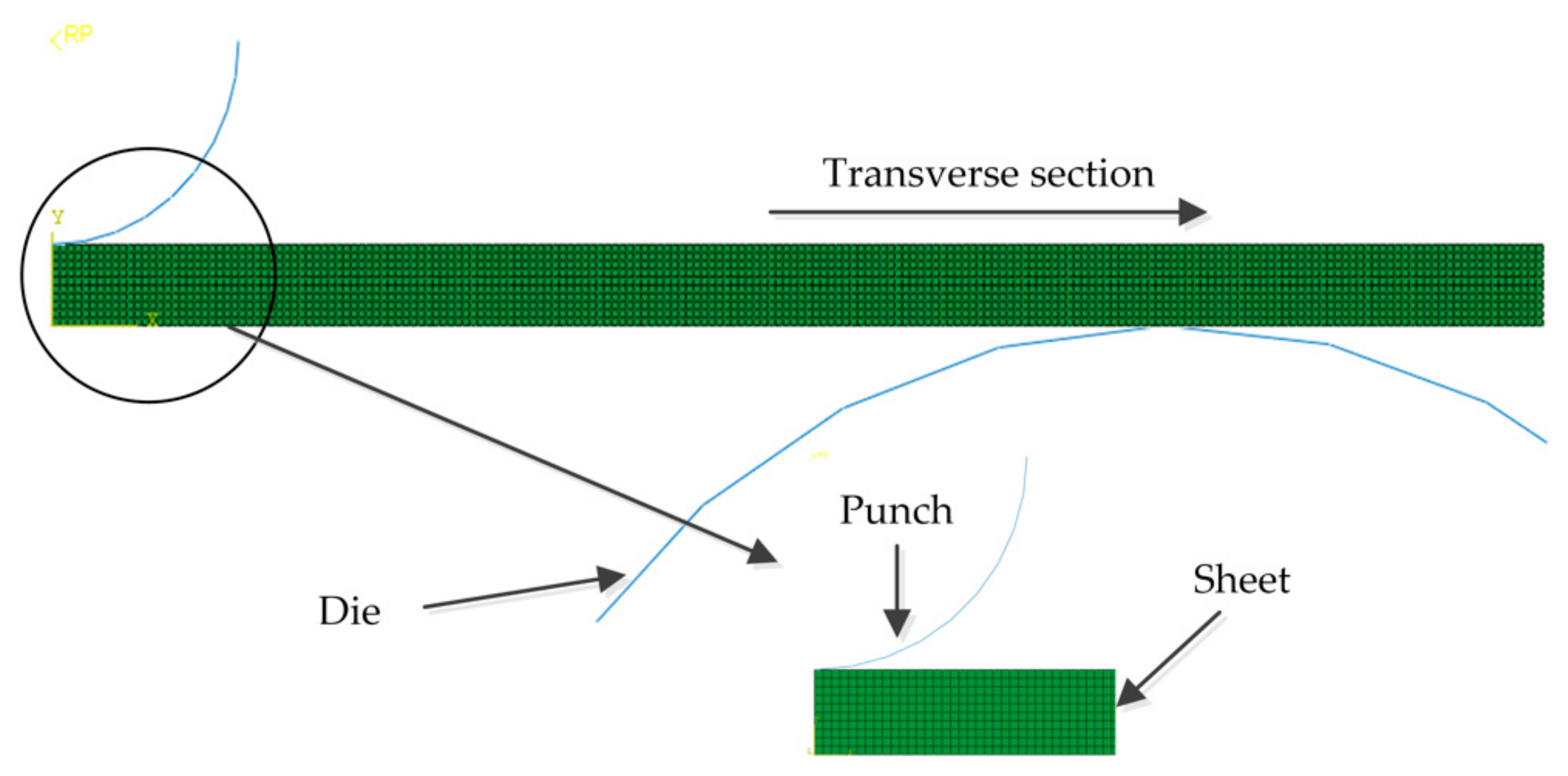
In the free V-bending test, the sheet metal is placed on two die columns, and then the punch moves downward to complete the test. The test device is shown in Figure 1, where rp is the punch fillet radius, rd is the die fillet radius, w is the die span, and the test device is able to adjust the die span. The force stroke curve extracted in the bending test will be affected by these three parameters. Under the same bending stroke and the same material, when one of these three parameters changes, the bending force will be affected, and then the shape of the whole force stroke curve will also be changed. The following section focuses on the analysis of the impact of these three parameters on the curve shape, and finds the best combination of geometric parameters of the test device for identifying the yield strength of the sheet.

2.1.1. Establishment of the Finite Element Model

To analyze the influence of different parameters on the force stroke curve, the finite element method was used to simulate and analyze the V-bending experiment. In ABAQUS (6.10 version, Dassault Systèmes Simulia Corp, Johnston, RI, USA), the implicit algorithm was used to establish the prediction model, which is shown in Figure 2. The punch and the die were set as the analytical rigid body, and the four-node plane strain element CPS4 was selected to mesh the sheet. The surface contact relationship was set between the upper surface of the punch and the sheet and between the lower bottom surface of the die and the sheet. The actual surfaces of the punch and the die were relatively smooth, so the friction coefficient was set as 0.05. To improve the stability and convergence of the model and reduce the rigid displacement of sheet, the reference point of the punch was set to have fixed boundary conditions, and the corresponding bending stroke was applied to the reference point of the die.

2.1.2. Stress–Strain Relationship

The Ramberg-Osgood equation was created to describe the nonlinear relation between stress and strain, especially the material property near yield points. This is useful for metals that harden with plastic deformation, showing a smooth elastic–plastic transition.
The Ramberg-Osgood model was used to describe the plastic stress–strain relationship of the materials, where Formula (2) is the calculation method of the hardening index. For example, Calaf-Chica used this equation and the small punch test to identify the parameters of materials; by setting the corresponding yield parameter and elastic modulus, the hardening index of materials can be calculated as follows:
ε = σ E + ε o f f s e t σ σ y n
n = ln ε m σ m / E ε o f f s e t ln σ m σ y
where εoffset is the offset strain, n is the hardening index, and σy is the yield parameter of the sheet. E is the elastic modulus. To analyze the influence of different material parameters on the force stroke curve, two materials of high yield and low yield were selected for comparative analysis. To facilitate subsequent analysis, they were marked as MYH and MYL, respectively. The elastic modulus of the two materials is 200 GPa, Poisson’s ratio is 0.3, n is 6.95, and εoffset remains unchanged at 0.002. Their yield stresses are 100 MPa and 1400 MPa, respectively. These two hypothetical materials were used to analyze the shape changes of the force stroke curve.

2.1.3. Influence of Test Device Geometric Parameters on Curve Shape

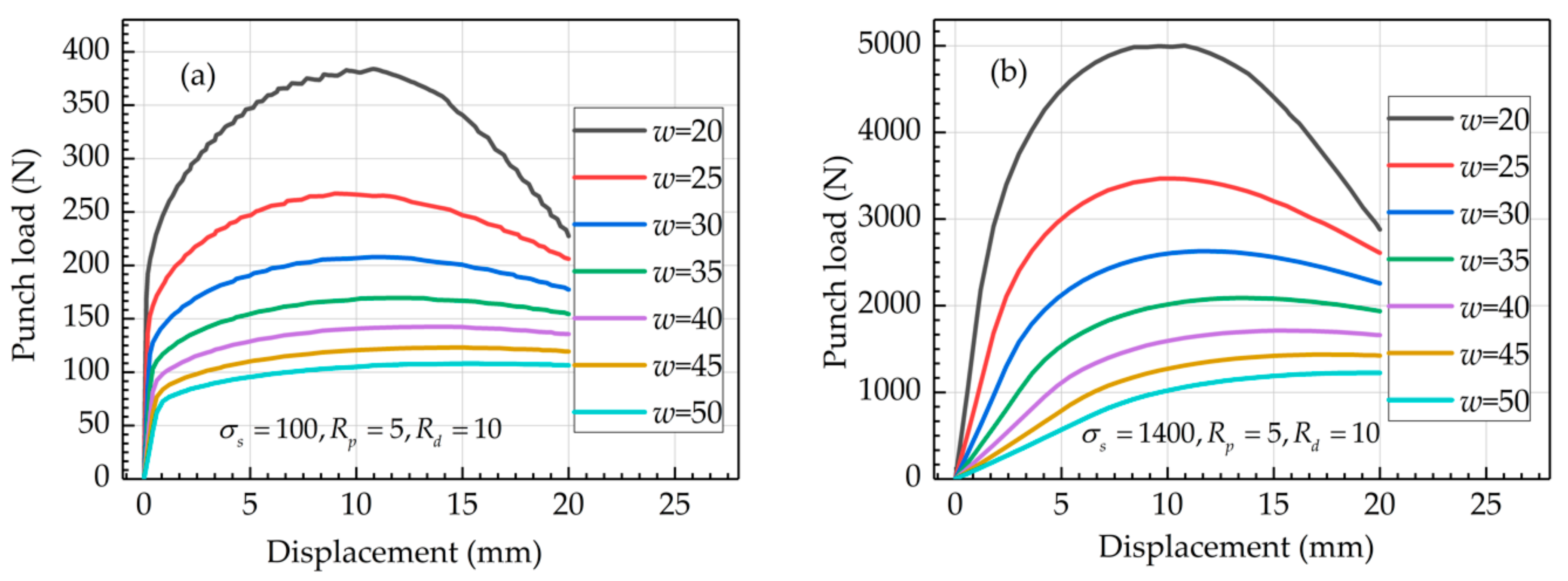
To analyze the influence of different span on the curve shape, the punch with a fillet radius of 5 mm and the die fillet radius of 10 mm was used to perform bending experiments on the sheet. The die span was between 20 and 50 mm. The bending force stroke curves of the MYL and MYH material under different spans is shown in Figure 3a,b, respectively. As can be seen from the curves in the figure, there are linear and non-linear turning points in the curve under different die spans. As the stroke increases, the curve gradually decreases after reaching the peak point. When the span is 20 mm, the linear and non-linear turning points and peak points of the curve are the highest, while when the span is 50 mm, the linear and non-linear turning points and peak points of the curve are the lowest. With the increase of the die span, the difference between the turning point and the peak point gradually becomes smaller. The overall shapes of the MYH and MYL curves at different spans are similar. The stroke of the peak point is similar, but the stroke of the linear and nonlinear turning points on the curve increases, the distance between the turning point and the peak point decreases, and the curvature of the transition stage of curve decreases. Therefore, the curve turns significantly with the greater span before and after the turning points, but bending experiments using a large span require longer specimens.
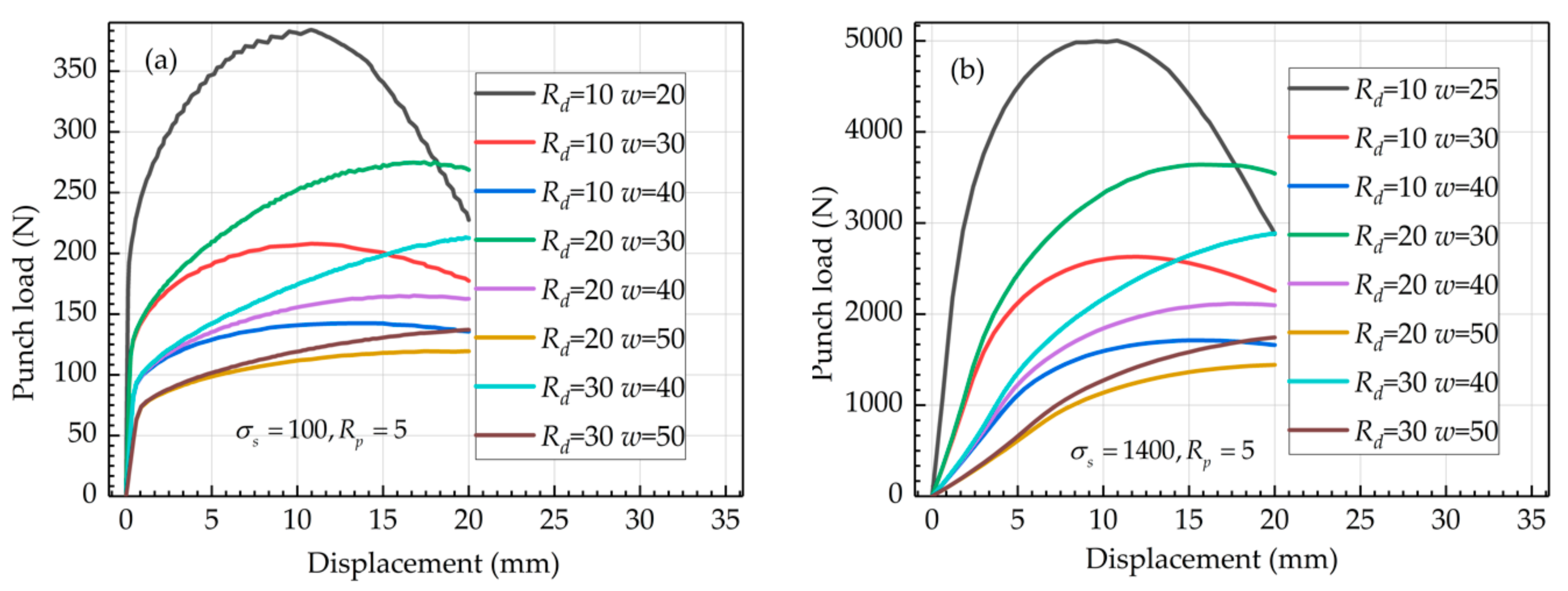
To analyze the influence of different die fillet radii on the bending curve, there are several curves with different die fillet radii under different spans shown in Figure 4, and the die fillet radii are selected from three sets of 10 mm, 20 mm, and 30 mm. It can be seen in Figure 4 that the die span is 30 mm, 40 mm, and 50 mm. With the same die span, the bending curve exhibits small differences before the turning points. However, after the turning points, the differences gradually increase with the increase of stroke. Additionally, with the same span, increasing the die fillet radius will lift the force stroke curve, and the peak point will move forward. From the groups of 10–30 mm, 20–40 mm, and 10–40 mm, 20–50 mm, when the die has different spans, the turning points of the curve will also be different. As the bending stroke increases, the actual inner span of the deformation gradually approaches, and the curve tail gradually approaches as well. It can be seen from the figure that the laws of the MYH materials are similar.
To analyze the influence of different punch radii on the bending curve, several curves with different punch fillets are shown in Figure 5. The punch fillet radius is selected from 5 mm, 6 mm, 7 mm, and 8 mm. It can be seen from Figure 5 that when the stroke is small, the sheet curvature radius under the punch is large, and the sheet is completely free to bend. In this state, there is no phenomenon of contact to the punch, and the difference of forming curves under different fillet radii is small. When the stroke is large, the sheet curvature radius below the punch gradually decreases. When it decreases to the same radius as the punch fillet, it will come into contact with the punch. The deformation resistance of the sheet after that will increase, and the curve will rise a little, but the range of increase is small. It can be seen from the comparison of Figure 5a,b that the rising point of the curve caused by this phenomenon is more advanced for materials with small yield stress, while the rising point of the curve for materials with higher yield stress is delayed.
In summary, if a longer length is allowed, the bending test device should be tested with a larger span, if possible. Increasing the die fillet radius can increase the force stroke curve after the turning points, reduce the degree of nonlinearity of the curve, and further improve the linear fitting correlation of the data, which is conducive to the recognition algorithm. When the sheet is deformed to a certain extent and sticks to the rounded corners of the punch, the force stroke curve can be slightly raised, but interaction between the punch and the sheet is introduced. Based on the above analysis, in the subsequent parameter identification experiments, a set of geometric parameters with a die span of 30 mm, a die fillet of 20 mm, and a punch fillet of 5 mm are selected.

2.2. Identification Algorithms and Materials

At present, some scholars have shown a linear relationship between yield load and yield strength of materials, which can be expressed by the following formula:
σ s = α 1 P y / t 2 + α 0
However, this method has the following problems:
  • The force stroke curve obtained by a given test device is a synthesis of material properties, and the yield load may be related to more material property parameters. To improve the prediction accuracy, the extracted yield load value should be more related to yield strength, reducing the influence of other parameters.
  • By comparing and analyzing the dispersion of different methods for yield strength prediction, a relatively stable recognition algorithm is determined. Combined with references and the characteristics of the bending force stroke curve, four methods are analyzed to explore the prediction accuracy and dispersion of yield strength.

2.2.1. t/10 Method [26]

The sheet thickness has a great influence on the force stroke curve. With the increase of the thickness, the corresponding yield load and yield stroke increase. This method refers to the method of the stress–strain curve in the uniaxial tensile experiment to determine the yield point, maintains the slope of the elastic stage line of the load curve without change, translates the line t/10 to the right, and takes the load at the intersection point of the new line and the load curve as the yield load. The typical determination process is shown in Figure 6.

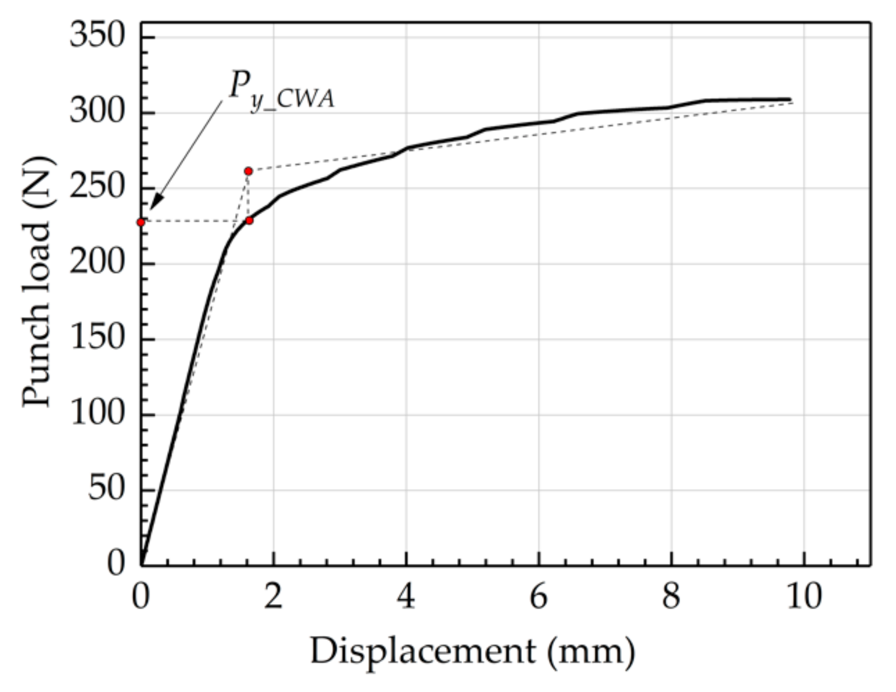
2.2.2. “Double Secant Line” Method (CWA [26])

The force stroke data before the maximum load point was extracted, and curves were drawn, as shown in Figure 7. Two straight lines were used for fitting before and after the turning point. The turning point coordinates were set as (hy, Py), and the fitting equation was constructed as follows:
P = P y h y h h h e k ( h h y ) + P y h h e
where the first line reflects the deformation behavior in the elastic stage, and the second line reflects the deformation behavior in the plastic stage. The intersection point Py of the two secant lines is the yield load. The least squares method is used to fit the above equations to minimize the errors.

2.2.3. Window Vector Method (WV)

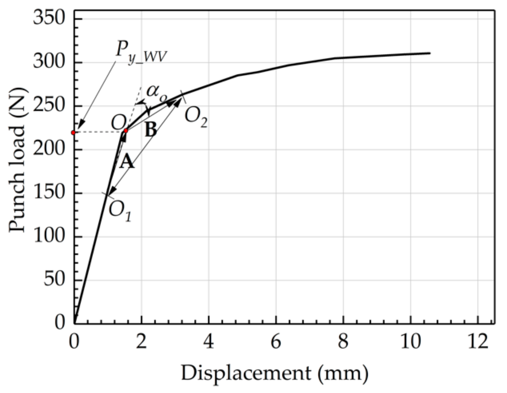
Firstly, the experimental data were filtered by least squares smoothing and normalized, and then the vector corner of the experimental data was extracted by window vector A and B. Then the vector corner data was filtered by least squares smoothing. Finally, the yield load Py at the maximum corner was extracted. The typical determination process is shown in Figure 8.

2.2.4. Fitting Residual Method (FR)

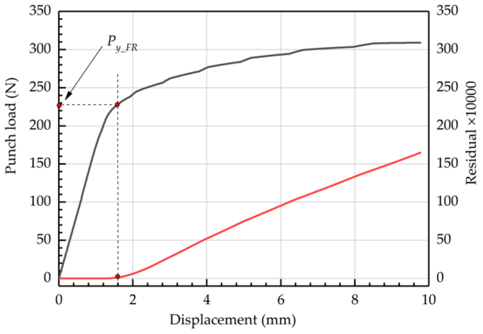
Firstly, the force stroke data was obtained as a continuous row data set, and then, starting from the third row, the data of the current row and the previous rows were linearly fitted, and a residual value was output at the current stroke point. The residual values of all the stroke points were drawn in a curve, as shown in Figure 9. When the residual value of the curve begins to increase, this indicates that the algorithm has been calculated at the turning point of force stroke curves. Therefore, the yield load is determined as shown in Figure 9.

2.2.5. Materials

To analyze the effectiveness of the algorithm, 36 hypothetical materials were suggested in the references [26], in which the elastic modulus E is assumed to be 200,000 MPa, and the Poisson’s ratio is 0.3. According to the yield strength, the materials are divided into nine material groups (100 MPa, 250 MPa, 400 MPa, 550 MPa, 700 MPa, 850 MPa, 1000 MPa, 1200 MPa, and 1400 MPa). Four Ramberg-Osgood coefficients n, namely, 6.95, 8.95, 14, and 35, were selected from each material group. All material parameter combinations are shown in Table 1. The ABAQUS finite element simulation model was established to predict the force stroke curve by using the above materials. In this paper, the isotropic constitutive model is selected for simulation, and the Ramberg-Osgood model was discretized into the identifiable hardening data by using the ABAQUS program, and the data was imported into software to complete the establishment of the finite element model.

3. Results

3.1. FEM Results

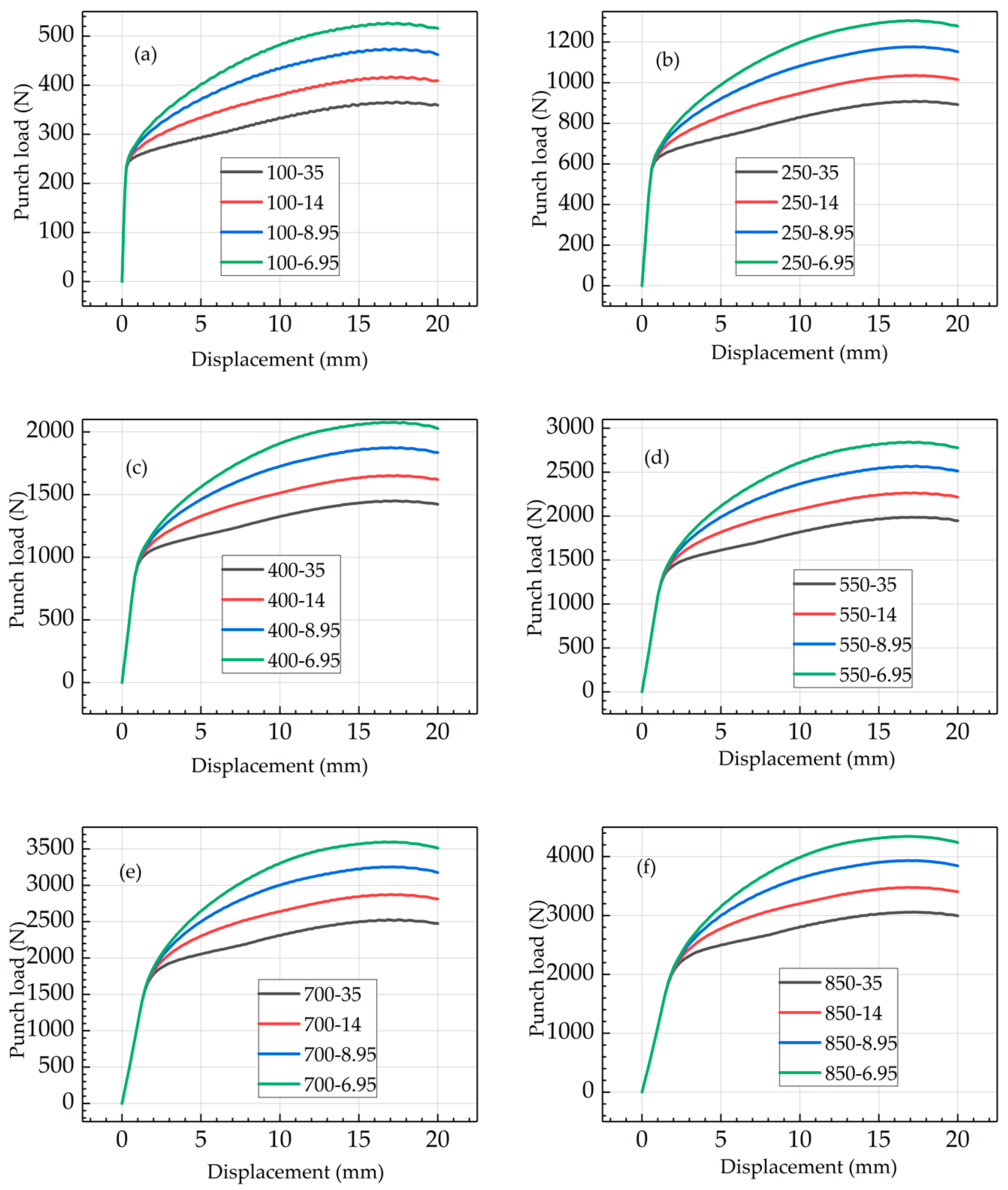
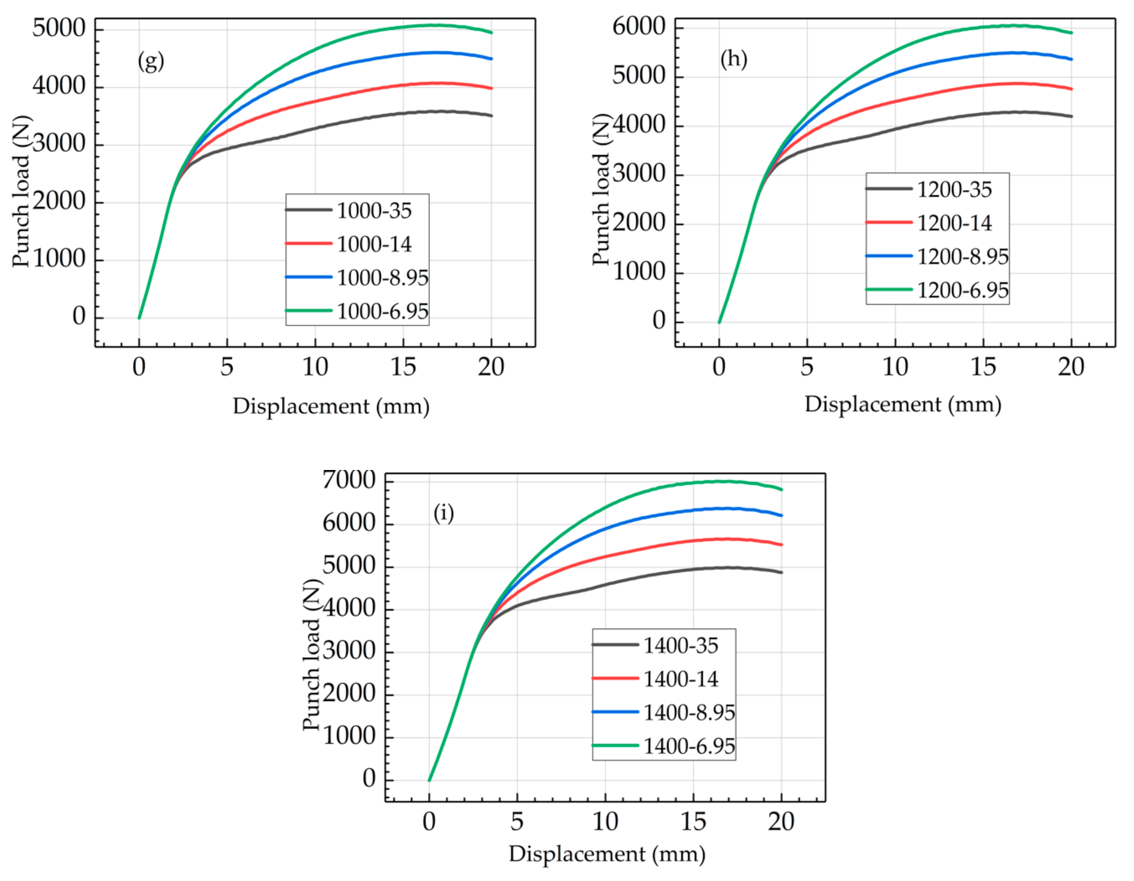
After the finite element calculation of 36 hypothetical materials M1.1–M9.4 had been completed, the result file of ABAQUS was processed. The load stroke curves of the four n are shown in Figure 10a when the yield strength is 100 MPa. It is obvious that the load curve increases gradually as the coefficient n decreases. After the turning point, the load curve increases and then decreases after reaching a peak point. When n decreases, the peak point increases, but the yield turning point of the curve remains unchanged, and the convexity of the curve increases. When the yield strength is 250 MPa, the load stroke curve under four n is shown in Figure 10b. It can be seen that when n is reduced, the overall change rule is similar to that of 100 MPa. The overall shape of the curve changes little, but the overall curve and the turning point both move up a certain distance. The load at the turning point is positively related to the stress in the material constitutive law. When the yield strength is 400 MPa, 550 MPa, 700 MPa, 850 MPa, 1000 MPa, 1200 MPa, and 1400 MPa, the curves are shown in Figure 10c–10i, respectively. With the increase of yield strength, the load at the turning point of the curve increases gradually, and the displacement at the turning point also increases. In the actual deformation, the increase of yield load and yield displacement on the curve is helpful for the algorithm to extract the characteristic data.
The above data were processed using the methods described in Section 3. To improve the comparability between sheets of different thicknesses and the objectivity of the data results, the load results were divided by the square value of corresponding sheet thickness. The results of 36 hypothetical materials are shown in Table 2.
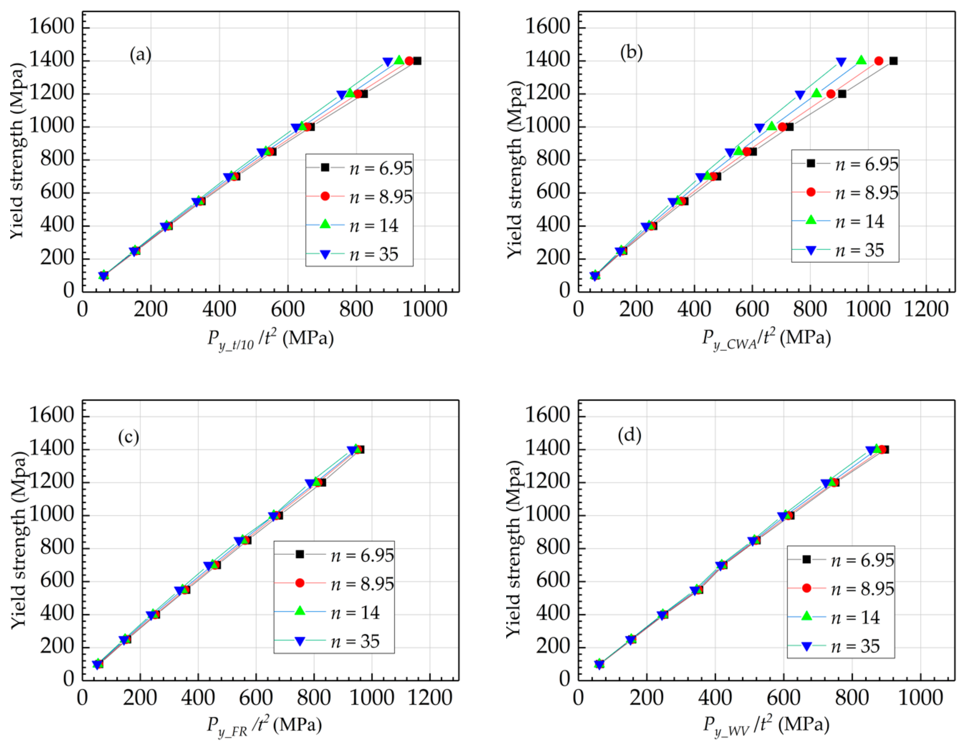
In Table 2, every four rows constitutes a group, and within one group, there are the predicted results of materials with the same yield strength and different Ramberg-Osgood coefficients n. To analyze the influence of different n on the prediction results, the relationship between yield load value and yield strength identified with different n was compared, as shown in Figure 11, where the relationship between yield load and yield strength identified by the t/10 method is shown in Figure 11a. It can be seen from Figure 11 that different n have certain influences on the identification of yield load. When the coefficient n increases, the yield load identified by this method decreases. It can be seen from Figure 11a that when the coefficient n increases, the force stroke curve moves down as a whole, and the curvature near the yield points increases, which will cause the load curve to drop slightly. This phenomenon will lead to a certain degree of dispersion of the identified results. When the yield strength is small, the t/10 method produces a dispersion value of about 2 MPa. Similarly, when the yield strength is large, the dispersibility increases, and its value is about 86 MPa. Compared with this method, the recognition result of the CWA method is shown in Figure 11b. It can be seen that when the coefficient n increases, the yield load value recognized by this method also decreases, and the law is similar to that of the t/10 method. When the yield strength is small, a dispersion value of 3 MPa is produced. When the yield strength is large, the dispersion value increases, with a value of about 181 MPa. The identification results of the FR method are shown in Figure 11c. When the Ramberg-Osgood coefficient n increases, the yield load value identified by this method also decreases, and the rule is similar to that of the above two methods. When the yield strength is small, a dispersion value of 7 MPa is produced. When the yield strength is large, the dispersion increases, with a value of about 29 MPa. It is obvious that when the yield strength becomes larger, the dispersion value decreases. The results of the WV method are shown in Figure 11d, which is the same as the above three methods. When the coefficient n increases, the yield load recognized by this method increases.
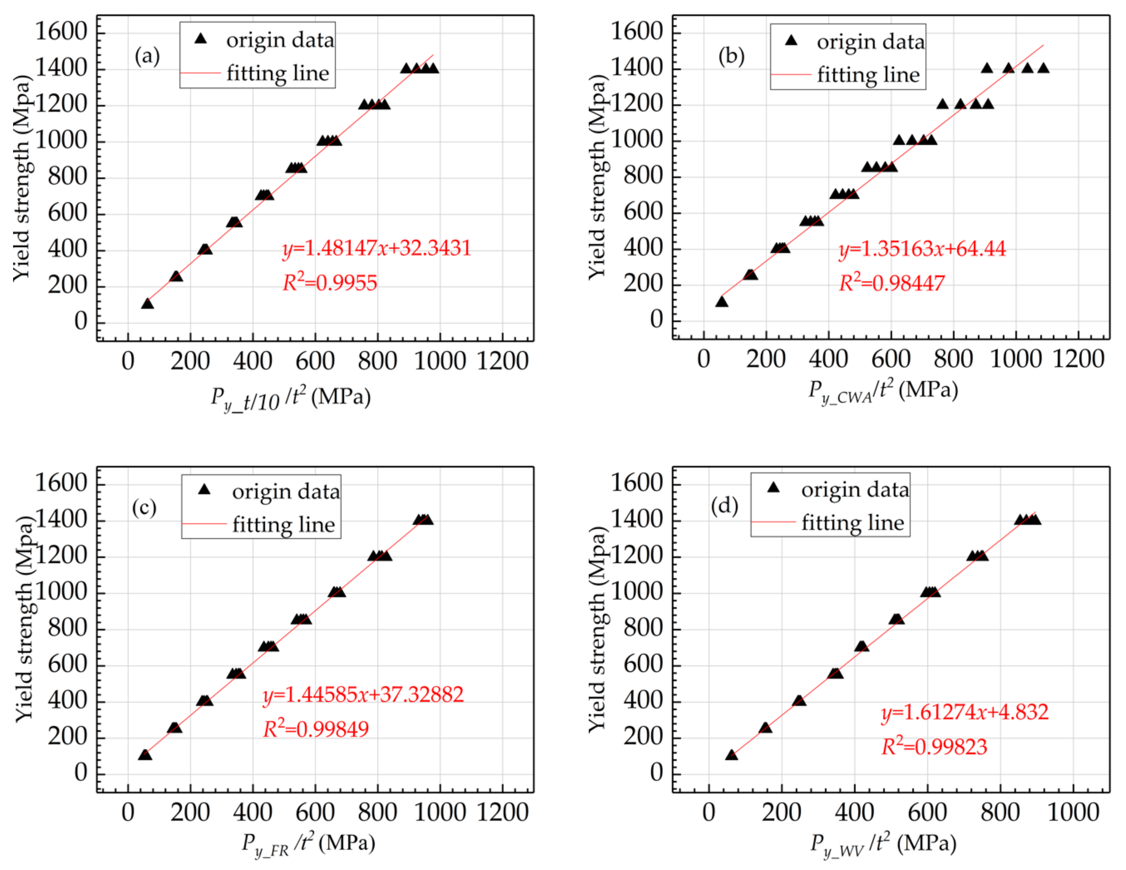
According to the data analysis of the above four methods, it can be concluded that the yield load determined by each method is positively related to the yield stress. Although it has a certain degree of dispersion, all yield strength and yield load can be regarded as approximately linear. After fitting Equation (1) using the least squares fitting method, the fitting curves were drawn using the t/10 method, CWA method, WV method, and FR method, as shown in Figure 12. The correlation coefficients of the fitted straight lines for each experimental data are shown in the figure. It can be seen that the correlation coefficients of the three methods of t/10, WV, and FR exceed 0.99, while the correlation coefficient of the CWA method is about 0.98, which is the lowest one, but the data fitting effect of this method is very good.
The fitting equations of yield load data identified by the four methods are presented as Equation (5), Equation (6), Equation (7), and Equation (8), respectively.
The fitting equation of the t/10 method:
σ y = 1.48147 P y t 2 + 32.3431
The fitting equation of the CWA method:
σ y = 1.35163 P y t 2 + 64.44
The fitting equation of the WV method:
σ y = 1.61274 P y t 2 + 4.832
The fitting equation of the FR method:
σ y = 1.44585 P y t 2 + 37.32882
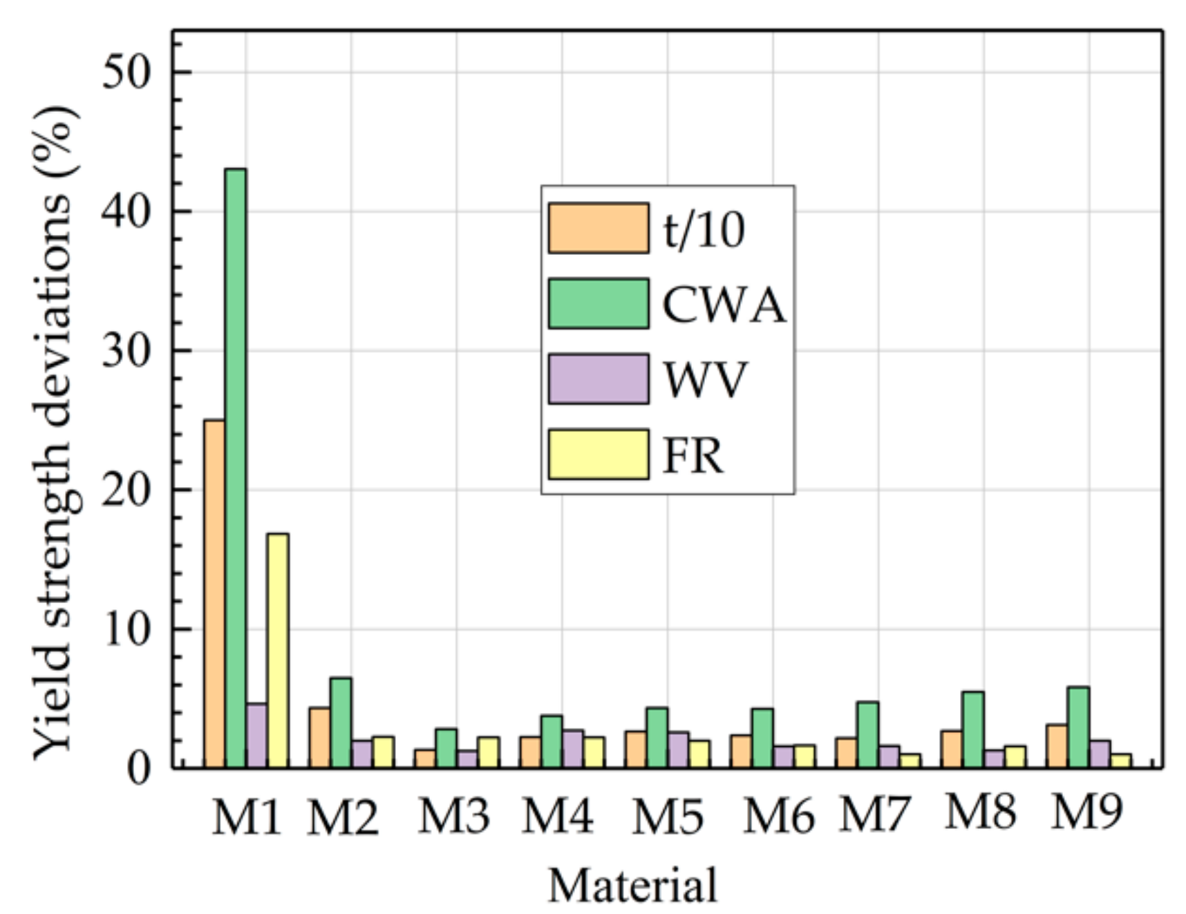
Figure 13 shows the average prediction errors of each method. It can be seen from the M1 group that the average error predicted by the four methods is higher than the average errors of other yield strengths. When the yield strength is small, the absolute value of the yield strength is low, and the slight dispersion will increase the average error. At the same time, when the yield strength is low, the elastic stroke is short, and a small stroke error will increase the prediction error in the elastic stage. When the stroke is small, the results are greatly affected by the interference factors. Among the eight materials M2–M9, the average yield strength error predicted by the four methods generally decreases, but the deviation results in an increase in yield strength. The overall prediction deviation is relatively stable in the eight materials M2–M9. The maximum point error of the t/10 method in the whole yield range is 4.1%, which appears in the M2 group. The maximum point error of the CWA method in this yield range is 6.3%, which also appears in the M2 group. Except for the M1 and M2 groups, the CWA prediction error increases with the increase of yield strength. The law of the t/10 method is irrelevant. The maximum point error of the WV method in the whole yield range is 2.3%, which appears in the M5 group. The maximum point error of the FR method in this yield range is 2.1%, which appears in the M4 group.

3.2. Experiment and Results

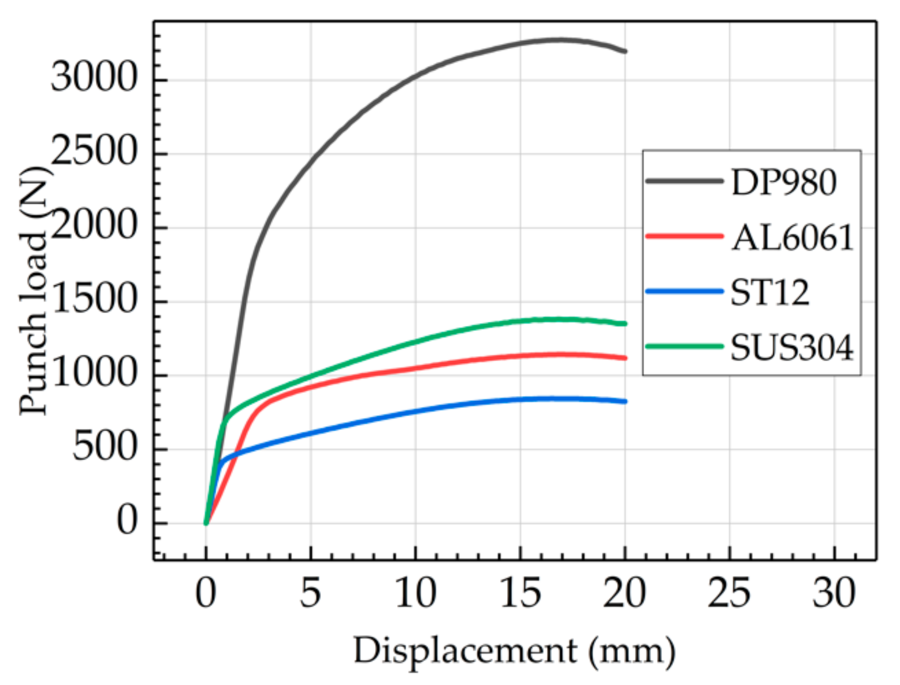
To verify the correctness of the above methods, four materials were selected for verification. The parameters of the four materials are shown in Table 3. The elastic modulus, yield strength, stress strength limit, and fracture strain are given. Among these materials, DP980 has a high yield, ST12 has a low yield and high plasticity, SUS304 and AL6061 have medium yields, and AL6061 is a non-ferrous metal. Their bending force stroke curves are shown in Figure 14. To increase the comparability between different materials, the curves of different materials are divided by their actual width, and then multiplied by 35 mm. It can be seen that DP980 has a higher yield load and a larger yield transition curve. For ST12, AL6061, and SUS304 sheets, their yield transition curves have a larger curvature and a faster transition. The comparisons of final yield prediction errors are shown in Table 3.
The above methods were used to test four experimental materials, and four methods were used to identify the data. The yield load data identified by different methods are shown in Table 4. The yield strength calculated by the above-mentioned linear equation is shown in Table 5. The first-order term coefficient of the above linear equation is greater than 1, and the constant term coefficient is greater than 0, so the yield load obtained in Table 4 is smaller than that in Table 5, and the yield load is relatively unchanged.
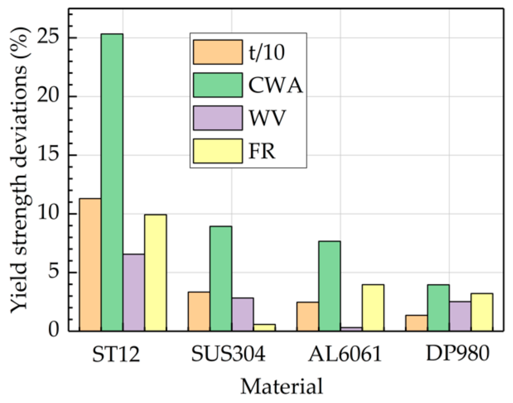
The yield strength calculated by the different methods described above was compared with the yield strength of the uniaxial tensile test data. The corresponding prediction deviations of the respective models are shown in Figure 15. It can be seen that when the material type changes, the predictive model deviation is different. Among them, ST12 has a low yield. When the prediction deviation is similar to other materials, the relative deviation is larger than other methods. The maximum error predicted by the CWA method for the ST12 is about 25%, and the minimum error predicted by the WV method is about 6%. In the comparison of the four methods, it is found that the prediction error by the CWA method is the largest, and the relative value of the predicted error changes with the change of materials. For materials with medium and high yields, the prediction errors by the three methods of t/10, WV, and FR are all below 4%, which can meet many technical and industrial requirements. The relevant model is simple in form, which can greatly improve the prediction efficiency and facilitate the embedding of chips to construct online sensors.

4. Conclusions

(1)
Based on the research on the geometric combination of the test device, it is concluded that the span of the bending test device should be selected to be as large as possible for experiments when the slab size allows. Increasing the fillet of the die can lift the force stroke curve, reduce the non-linear degree of the curve, and improve the linear fitting correlation of the data after the turning point, which is conducive to the recognition algorithm. When the metal sheet deforms to a certain extent and comes into contact with the punch fillet, the force stroke curve can be slightly increased, but interaction between the punch and the metal sheet is introduced. A group of geometric parameters, including a die span of 30 mm, a die fillet of 20 mm, and a punch fillet of 5 mm, was selected.
(2)
The WV method and FR method were proposed in this paper. In the WV method, the vector angle data of the experiment data are extracted by the window vector, and the yield load at the maximum angle is also extracted. In the FR method, the residual values at all points are output. The increase of the residual values means that the turning point of the force stroke curve has been reached. With CWA and t/10, the linear correlation between yield load and yield strength determined by the four methods is close to 0.99, while the WV method and FR method are relatively stable and easy to program.
(3)
When the yield strength and absolute value of yield strength are small, the average errors and the dispersion of related models will increase. At the same time, when the yield strength is low, and the elastic stroke is short, small stroke errors will increase the prediction errors in the elastic stage. When the stroke is small, the results are greatly affected by interference factors. With increasing yield strength, the deviation results increase gradually. For experimental materials with medium and high yields, the prediction errors of the correlation model identified by t/10, WV, and FR were less than 4%, and the prediction deviation was stable. The three methods have certain dispersion degrees, but these methods are relatively simple, and can be embedded in the data processing unit to develop an intelligent sensor for identifying yield strength.

Author Contributions

Y.D. conceived and designed the experiments, L.T. performed the experiments and built the software. F.Z. proved the validity. Y.D. wrote the original draft. Y.D. and L.T. reviewed and edited the article. Y.D., L.T. and H.Q. finished the visualization. M.L., L.Y. and Y.G. put forward suggestions for modification. Y.D., F.Z. and Y.G. provided project administration. All authors have read and agreed to the published version of the manuscript.

Funding

This research was funded by National Natural Science Foundation of China (51705448), Hebei Natural Science Foundation (E2018203100), Doctoral Foundation of Yanshan University (B861) and Youth Teachers Independent Research Foundation of Yanshan University (15LGB002).

Conflicts of Interest

The authors declare no conflict of interest. The funders had no role in the design of the study; in the collection, analyses, or interpretation of data; in the writing of the manuscript; or in the decision to publish the results.

References

  1. Yang, M.; Manabe, K.-I.; Nishimura, H. Development of Real-time Process Control System for Precision and Flexible V-bending with an On-line Database. J. Mater. Process. Technol. 1996, 60, 249–254. [Google Scholar] [CrossRef]
  2. Garcia-Romeu, M.L.; Ciurana, J.; Ferrer, I. Springback Determination of Sheet Metals in an Air Bending Process Based on an Experimental Work. J. Mater. Process. Technol. 2007, 191, 174–177. [Google Scholar] [CrossRef]
  3. Karbasian, H.; Tekkaya, A.E. A Review on Hot Stamping. J. Mater. Process. Technol. 2010, 210, 2103–2118. [Google Scholar] [CrossRef]
  4. Suppan, C.; Hebesberger, T.; Pichler, A.; Rehrl, J.; Kolednik, O. On the Microstructure Control of the Bendability of Advanced High Strength Steels. Mater. Sci. Eng. A 2018, 735, 89–98. [Google Scholar] [CrossRef]
  5. Albakri, M.; Fadi, A.; Khraisheh, M. A New Combined Experimental–Numerical Approach to Evaluate Formability of Rate Dependent Materials. Int. J. Mech. Sci. 2013, 66, 55–66. [Google Scholar] [CrossRef]
  6. Kaupper, M.; Merklein, M. Bendability of advanced high strength steels—A new evaluation procedure. CIRP Ann. Manuf. Techn. 2013, 62, 247–250. [Google Scholar] [CrossRef]
  7. Rèche, D.; Sturel, T.; Bouaziz, O.; Col, A.; Gourgues-Lorenzon, A.F. Damage Development in Low Alloy TRIP-aided Steels during Air-bending. Mater. Sci. Eng. A 2011, 528, 5241–5250. [Google Scholar] [CrossRef]
  8. Pradeau, A.; Thuillier, S.; Yoon, J.W. Prediction of Failure in Bending of an Aluminium Sheet Alloy. Int. J. Mech. Sci. 2016, 119, 23–35. [Google Scholar] [CrossRef]
  9. Mattei, L.; Daniel, D.; Guiglionda, G.; Klöcker, H.; Driver, J. Strain Localization and Damage Mechanisms during Bending of AA6016 Sheet. Mater. Sci. Eng. A 2013, 559, 812–821. [Google Scholar] [CrossRef]
  10. Lin, G.; Hu, S.; Cai, W. Evaluation of Formability in Bending/Hemming of Aluminum Alloys Using Plane-Strain Tensile Tests. J. Manuf. Sci. Eng. 2009, 131, 051009. [Google Scholar] [CrossRef]
  11. Yang, D.Y.; Bambach, M.; Cao, J.; Duflou, J.R.; Groche, P.; Kuboki, T.; Sterzing, A.; Tekkaya, A.E.; Lee, C.W. Flexibility in Metal Forming. CIRP Ann. Manuf. Techn. 2018, 67, 743–765. [Google Scholar] [CrossRef]
  12. Ha, J.; Lee, M.-G.; Barlat, F. Strain Hardening Response and Modeling of EDDQ and DP780 Steel Sheet under Non-linear Strain Path. Mech. Mater. 2013, 64, 11–26. [Google Scholar] [CrossRef]
  13. Havinga, J.; Boogaard, T.; Dallinger, F.; Hora, P. Feedforward Control of Sheet Bending Based on Force Measurements. J. Manuf. Process. 2018, 31, 260–272. [Google Scholar] [CrossRef]
  14. Bruschi, S.; Altan, T.; Banabic, D.; Bariani, P.F.; Brosius, A.; Cao, J.; Ghiotti, A.; Khraisheh, M.; Merklein, M.; Tekkaya, A.E. Testing and Modelling of Material Behaviour and Formability in Sheet Metal Forming. CIRP Ann. Manuf. Techn. 2014, 63, 727–749. [Google Scholar] [CrossRef]
  15. Canteli, J.A.; Cantero, J.L.; Miguélez, M.H. Experimental Identification of a Thermo-mechanical Model for Air Bending. J. Mater. Process. Technol. 2008, 203, 267–276. [Google Scholar] [CrossRef] [Green Version]
  16. An, Y.G.; Vegter, H.; Heijne, J. Development of Simple Shear Test for the Measurement of Work Hardening. J. Mater. Process. Technol. 2009, 209, 4248–4254. [Google Scholar] [CrossRef]
  17. Allwood, J.M.; Duncan, S.R.; Cao, J.; Groche, P.; Hirt, G.; Kinsey, B.; Kuboki, T.; Liewald, M.; Sterzing, A.; Tekkaya, A.E. Closed-loop Control of Product Properties in Metal Forming. CIRP Ann. Manuf. Techn. 2016, 65, 573–596. [Google Scholar] [CrossRef] [Green Version]
  18. Yang, M. Smart Metal Forming with Digital Process and IoT. Int. J. Lightweight Mater. Manuf. 2018, 1, 207–214. [Google Scholar] [CrossRef]
  19. Simons, G.; Weippert, C.; Dual, J.; Villain, J. Size Effects in Tensile Testing of Thin Cold Rolled and Annealed Cu Foils. Mater. Sci. Eng. A 2006, 4196, 290–299. [Google Scholar] [CrossRef]
  20. Nasser, A.; Yadav, A.; Pathak, P.; Altan, T. Determination of the flow stress of five AHSS sheet materials (DP 600, DP 780, DP 780-CR, DP 780-HY and TRIP 780) using the uniaxial tensile and the biaxial Viscous Pressure Bulge (VPB) tests. J. Mater. Process. Technol. 2010, 210, 429–436. [Google Scholar] [CrossRef]
  21. Hannon, A.; Tiernan, P. A Review of Planar Biaxial Tensile Test Systems for Sheet Metal. J. Mater. Process. Technol. 2008, 198, 1–13. [Google Scholar] [CrossRef]
  22. Lecompte, D.; Smits, A.; Sol, H.; Vantomme, J.; Hemelrijck, D.V. Mixed Numerical–Experimental Technique for Orthotropic Parameter Identification Using Biaxial Tensile Tests on Cruciform Specimens. Int. J. Solids Struct. 2007, 44, 1643–1656. [Google Scholar] [CrossRef] [Green Version]
  23. Merklein, M.; Biasutti, M. Development of a Biaxial Tensile Machine for Characterization of Sheet Metals. J. Mater. Process. Technol. 2013, 213, 939–946. [Google Scholar] [CrossRef]
  24. Abu-Farha, F.; Hector, L.G., Jr.; Khraisheh, M. Cruciform-shaped Specimens for Elevated Temperature Biaxial Testing of Lightweight Materials. JOM 2009, 61, 48–56. [Google Scholar] [CrossRef]
  25. Calaf-Chica, J.; Díez, P.M.B.; Calzada, M.P. Improved Correlation for Elastic Modulus Prediction of Metallic Materials in the Small Punch Test. Int. J. Mech. Sci. 2017, 134, 112–122. [Google Scholar] [CrossRef]
  26. Calaf-Chica, J.; Díez, P.M.B.; Calzada, M.P. Development of an Improved Prediction Method for the Yield Strength of Steel Alloys in the Small Punch Test. Mater. Des. 2018, 148, 153–166. [Google Scholar] [CrossRef] [Green Version]
  27. Priel, E.; Mittelman, B.; Haroush, S.; Turgeman, A.; Shneck, R.; Gelbstein, Y. Estimation of Yield and Ultimate Stress Using the Small Punch Test Method Applied to Non-standard Specimens: A Computational Study Validated by Experiments. Int. J. Mech. Sci. 2018, 135, 484–498. [Google Scholar] [CrossRef]
  28. Calaf-Chica, J.; Díez, P.M.B.; Calzada, M.P.; Ballorca-Juez, D. A Systematic FEM Analysis of the Influence of Mechanical Properties in the Reliability of the Correlation Methods in the Small Punch Test. Int. J. Mech. Sci. 2019, 153–154, 299–309. [Google Scholar] [CrossRef]
  29. Lloyd, D.J.; Evans, D.; Pelow, C.; Nolan, P.; Jain, M. Bending in Aluminium Alloys AA 6111 and AA 5754 Using the Cantilever Bend Test. Mater. Sci. Technol. 2002, 18, 621–628. [Google Scholar] [CrossRef]
  30. Mattei, L.; Daniel, D.; Guiglionda, G.; Moulin, N.; Klöcker, H.; Driver, J. Grain Scale Modeling of the Bendability of AA6xxx Al Alloy Sheet. Mater. Sci. Technol. A 2013, 583, 96–104. [Google Scholar] [CrossRef]
  31. Triantafyllidis, N.; Needleman, A.; Tvergaard, V. On the Development of Shear Bands in Pure Bending. Int. J. Solids Struct. 1982, 18, 121–138. [Google Scholar] [CrossRef]
  32. Muhammad, W.; Kang, J.; Brahme, A.P.; Ali, U.; Hirsch, J.; Brinkman, H.-J.; Engler, O.; Mishra, R.K.; Inal, K. Bendability Enhancement of an Age-hardenable Aluminum Alloy: Part I—Relationship Between Microstructure, Plastic Deformation and Fracture. Mater. Sci. Eng. A 2019, 753, 179–191. [Google Scholar] [CrossRef]
  33. Groche, P.; Hoppe, F.; Hesse, D.; Calmano, S. Blanking-bending Process Chain with Disturbance Feed-forward and Closed-loop Control. J. Manuf. Process. 2016, 24, 62–70. [Google Scholar] [CrossRef]
  34. Wang, J.; Verma, S.; Alexander, R.; Gau, J. Springback Control of Sheet Metal Air Bending Process. J. Manuf. Process. 2008, 10, 21–27. [Google Scholar] [CrossRef]
  35. Imai, K.; Koyama, J.; Jin, Y. High-accuracy V-bending System by Real Time Identifying Material Property. J. Mater. Process. Technol. 2008, 201, 193–197. [Google Scholar] [CrossRef]
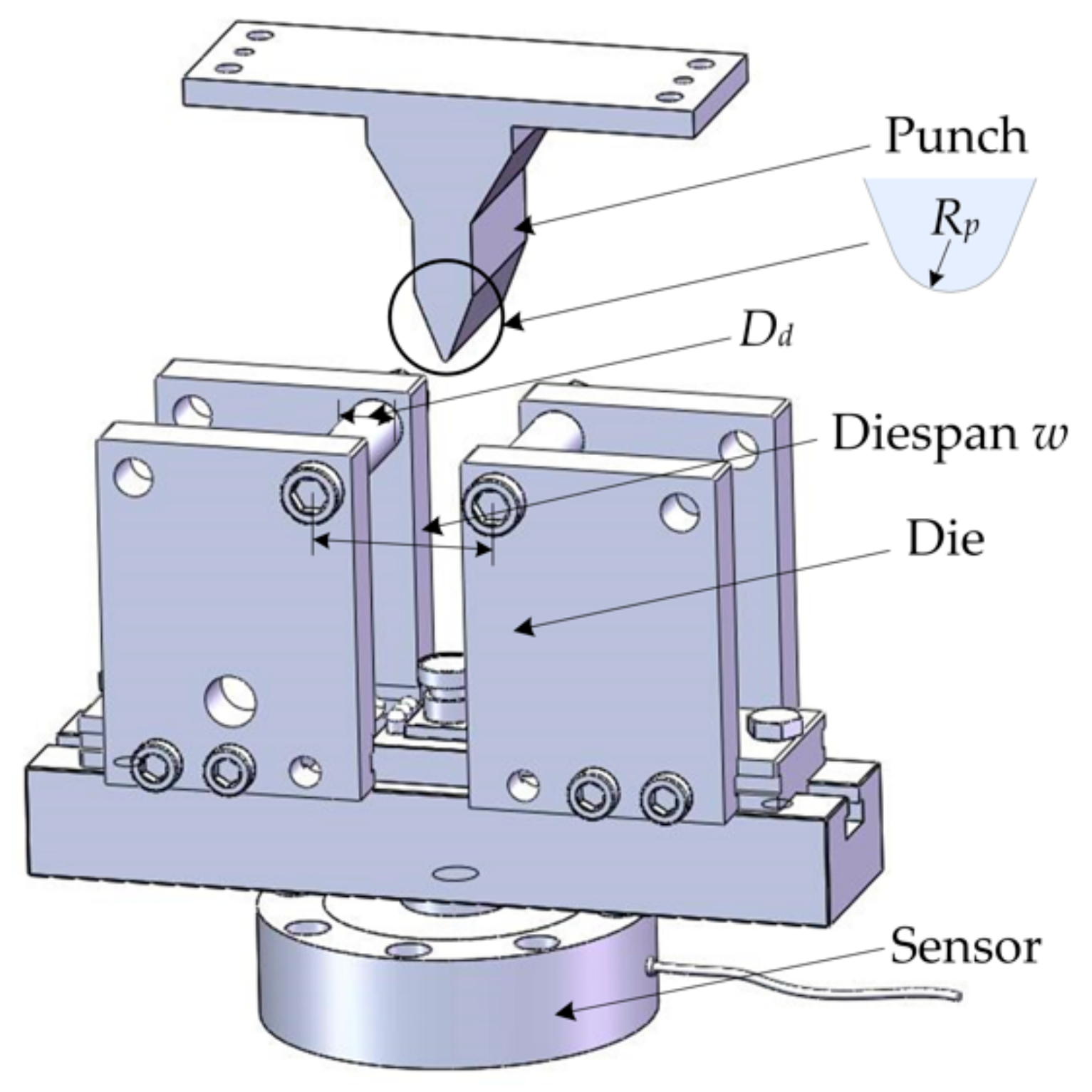
Figure 1. Bending test device.
Metals 10 00169 g001
Figure 2. Finite element prediction model.
Metals 10 00169 g002
Figure 3. Stroke curve of bending force under different die spans: (a) MYL; (b) MYH.
Metals 10 00169 g003
Figure 4. Stroke curve of bending force under different spans and different die fillets: (a) MYL; (b) MYH.
Metals 10 00169 g004
Figure 5. Stroke curve of bending force under different punch fillets: (a) MYL; (b) MYH.
Metals 10 00169 g005
Figure 6. t/10 method.
Metals 10 00169 g006
Figure 7. CWA method.
Metals 10 00169 g007
Figure 8. WV method.
Metals 10 00169 g008
Figure 9. FR method.
Metals 10 00169 g009
Figure 10. Bending force stroke curve of hypothetical materials: (a) 100MPa; (b) 250MPa (c) 400MPa; (d) 550MPa; (e) 700MPa; (f) 850MPa; (g) 1000MPa; (h) 1200MPa; (i) 1400MPa.
Metals 10 00169 g010aMetals 10 00169 g010b
Figure 11. Linear correlation of yield loads identified by different identification methods: (a) t/10 method; (b) CWA method; (c) FR method; (d) WV method.
Metals 10 00169 g011
Figure 12. Linear fit results of yield load: (a) t/10 method; (b) CWA method; (c) FR method; (d) WV method.
Metals 10 00169 g012
Figure 13. Deviation results of yield load identified by different methods.
Metals 10 00169 g013
Figure 14. Curve of bending force stroke of experimental material.
Metals 10 00169 g014
Figure 15. Deviation results of experimental materials.
Metals 10 00169 g015
Table 1. Plastic parameters of hypothetical materials.
MaterialσynMaterialσyn
M1.11006.95M5.370014
M1.21008.95M5.470035
M1.310014M6.18506.95
M1.410035M6.28508.95
M2.12506.95M6.385014
M2.22508.95M6.485035
M2.325014M7.110006.95
M2.425035M7.210008.95
M3.14006.95M7.3100014
M3.24008.95M7.4100035
M3.340014M8.112006.95
M3.440035M8.212008.95
M4.15506.95M8.3120014
M4.25508.95M8.4120035
M4.355014M9.114006.95
M4.455035M9.214008.95
M5.17006.95M9.3140014
M5.27008.95M9.4140035
Table 2. Different identification methods to identify the value of assumed materials.
MaterialsPy_t/10/t2Py_CWA/t2Py_WV/t2Py_FR/t2
M1.163.67059.38463.20058.469
M1.263.04959.06861.88156.521
M1.362.24557.93861.32653.828
M1.461.23956.23961.14351.190
M2.1157.339154.856157.601154.776
M2.2155.596151.449156.273151.025
M2.3153.336147.447154.440147.421
M2.4150.741143.425152.144143.291
M3.1251.980258.273251.048254.551
M3.2249.161251.467249.135250.763
M3.3245.495243.404246.442243.561
M3.4241.273232.827244.105237.132
M4.1348.183366.090353.198359.187
M4.2344.080355.656350.150353.870
M4.3338.893342.016345.832345.832
M4.4333.220325.486340.094334.851
M5.1449.285478.987423.818464.773
M5.2442.928463.712421.715457.958
M5.3434.608444.233418.768449.394
M5.4425.945421.639415.045435.425
M6.1555.185602.048520.999570.253
M6.2546.093580.645518.190561.749
M6.3535.143552.733514.202553.219
M6.4523.490523.278509.204540.457
M7.1666.760728.723619.960679.210
M7.2655.263703.819613.107669.076
M7.3640.240666.674604.958660.799
M7.4623.248625.139596.146659.155
M8.1821.853910.292751.325828.698
M8.2803.385871.368747.236813.340
M8.3781.660821.763737.344805.343
M8.4756.738764.815722.822786.348
M9.1977.6951087.497895.839960.197
M9.2954.1251036.608886.443950.362
M9.3924.463975.898870.769944.653
M9.4891.603906.794853.902931.266
Table 3. Mechanical properties of experimental materials.
MaterialsE(MPa)σy(MPa)σu_eng (MPa)ɛfractt(mm)
DP98014145074011280.1812.02
Al6061571843113670.1201.98
SUS30416991428615830.8201.96
ST121230001714400.4292.06
Table 4. Yield load of experimental materials identified by different identification methods.
MaterialsPy_t/10/t2Py_CWA/t2Py_WV/t2Py_FR/t2
DP980470.934521.450467.428502.437
Al6061193.287200.063190.440197.805
SUS304177.669182.823179.353173.126
ST12106.656110.878109.985104.198
Table 5. Yield strength predicted by different identification methods.
Materialsσy_t/10σy_CWAσy_WVσy_FR
DP980729.997769.247758.672763.777
Al6061318.673334.851311.963323.325
SUS304295.535311.549294.081287.643
ST12190.331214.306182.209187.984