Degassing Rhythms and Fluctuations of Geogenic Gases in A Red Wood-Ant Nest and in Soil in The Neuwied Basin (East Eifel Volcanic Field, Germany)


Abstract
1. Introduction
2. Methods
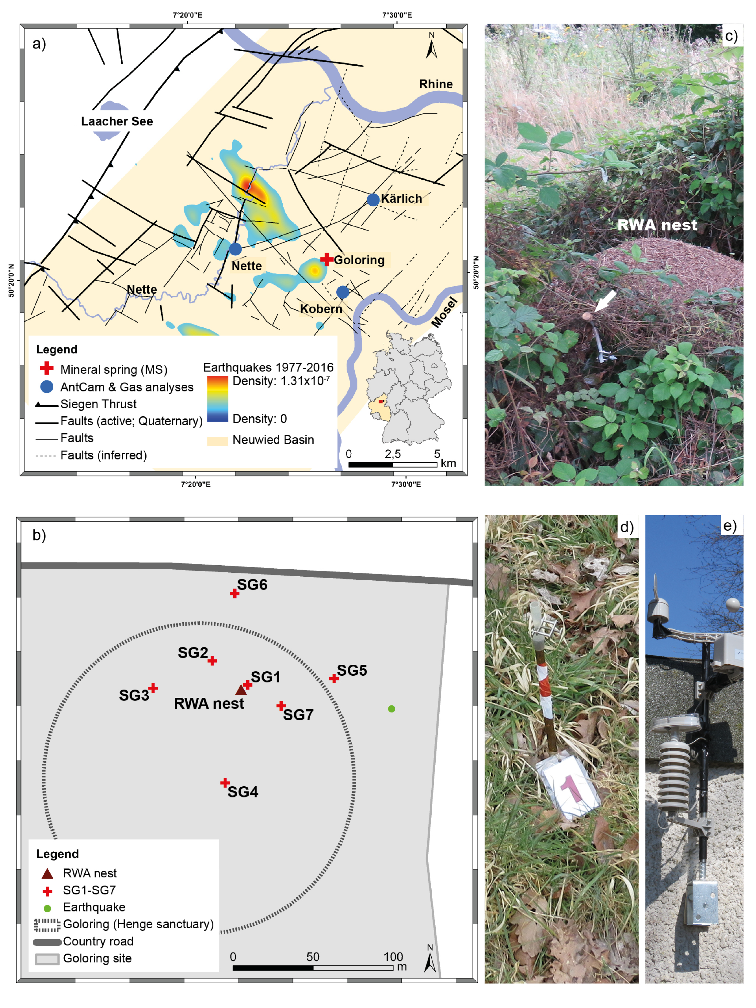
2.1. Study Area
2.2. Gas Sampling and Geochemical Analyses
2.3. External Factors
2.4. Data Analysis
2.5. Availability of Data
3. Results
3.1. Gases in Ambient Air, Soil, and the RWA Nest
3.1.1. CO2
3.1.2. He
3.1.3. Rn
3.2. Time Series
3.2.1. Fluctuations in Gas Concentrations
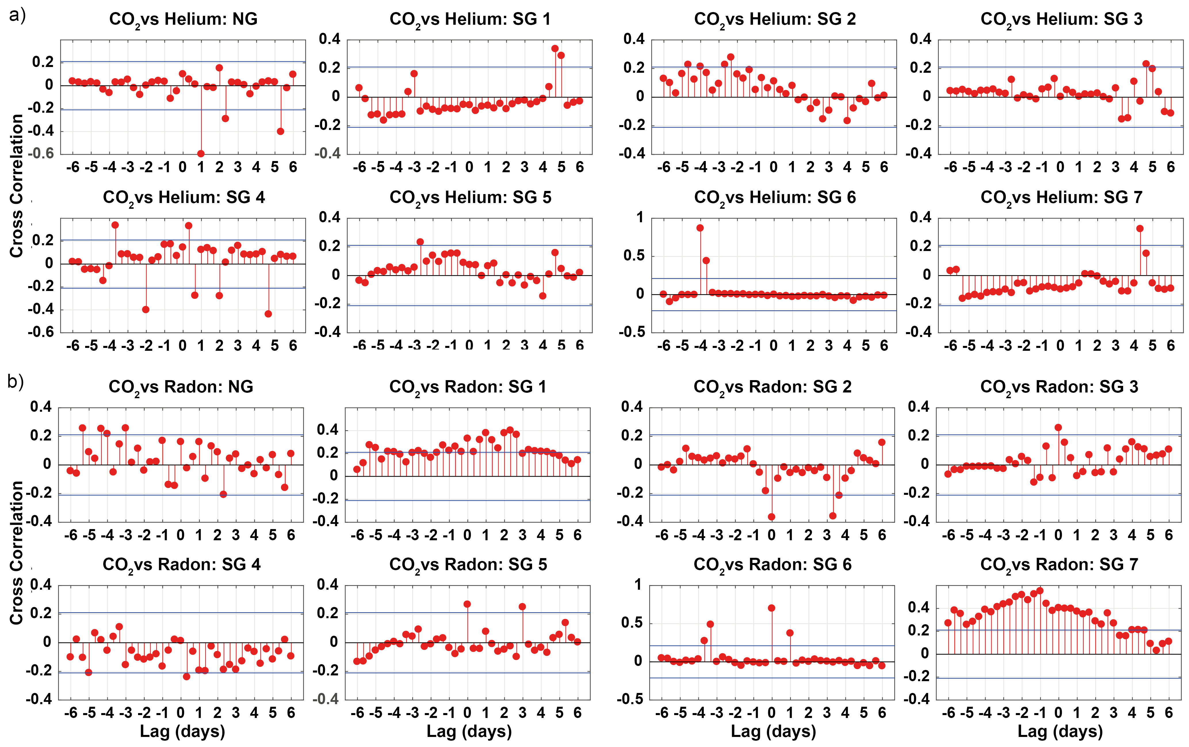
3.2.2. Temporal Variations of Concentrations and Carrier-Trace Gas Couples in SG and NG
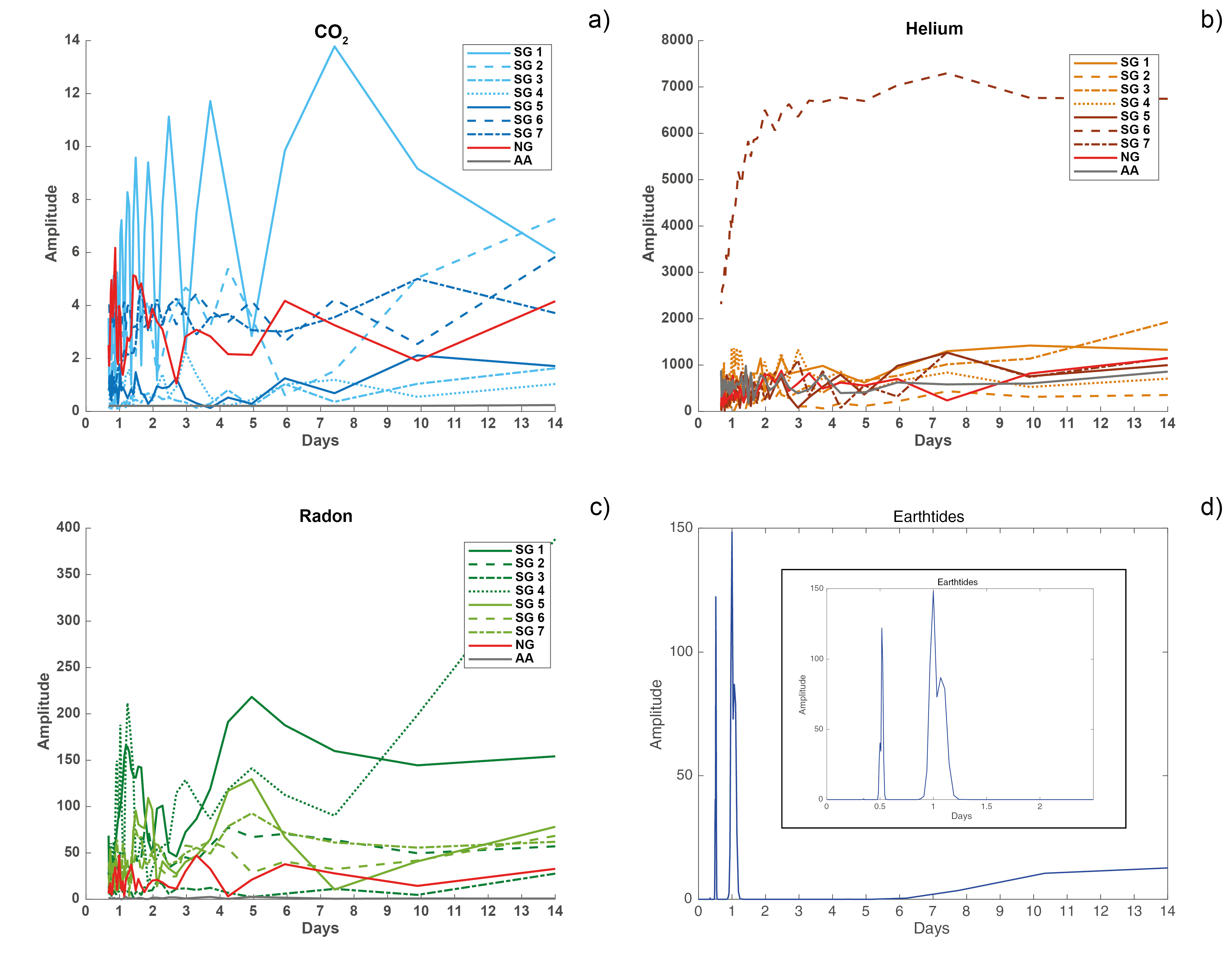
3.2.3. Fourier Analysis
3.3. External Factors
4. Discussion
4.1. Gases in Ambient Air, Nest and Soil
4.1.1. CO2
4.1.2. He
4.1.3. Rn
4.2. Time Series
4.3. External Factors
4.3.1. Meteorological Conditions
4.3.2. Earthquakes
4.3.3. Earth tides
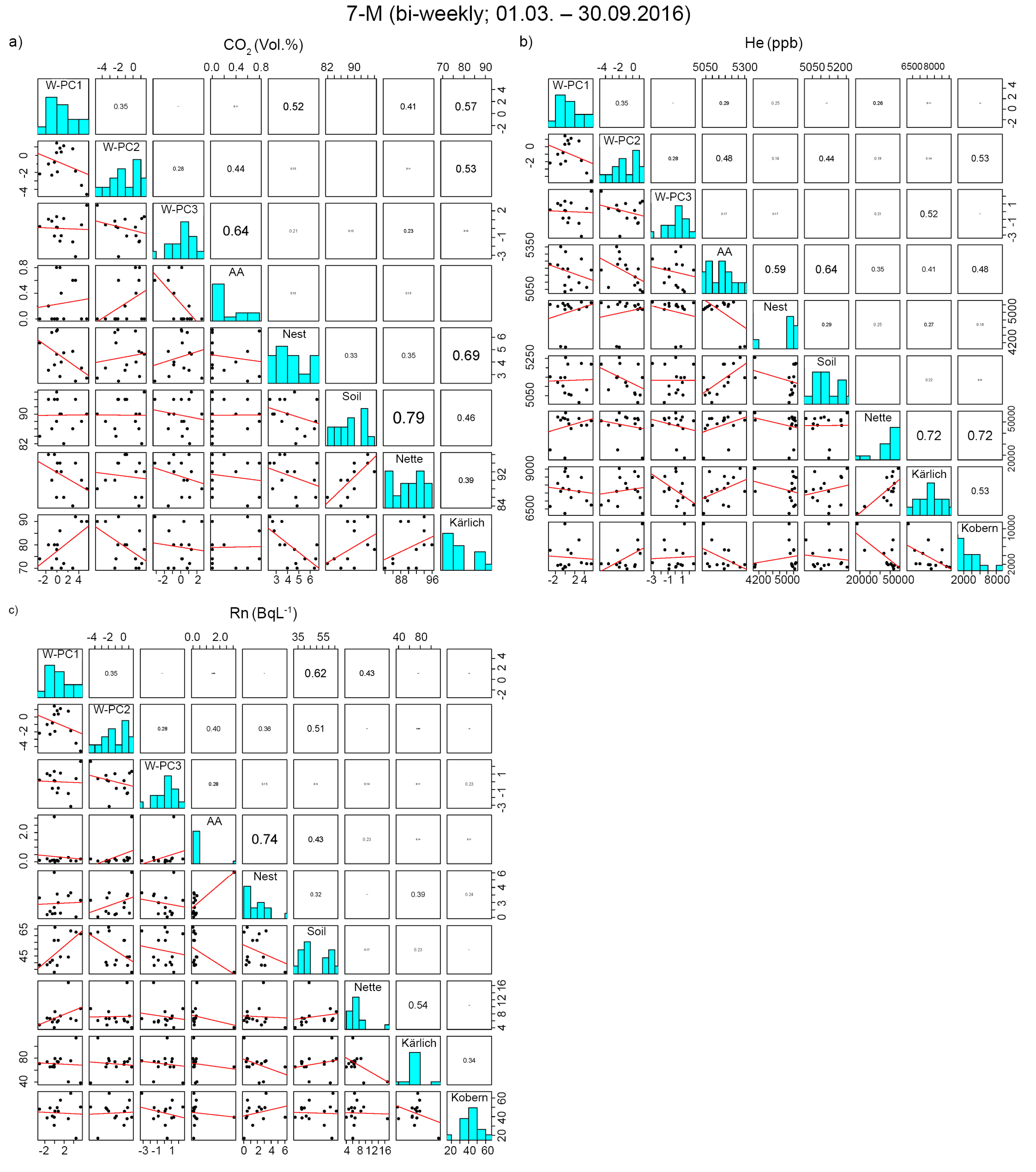
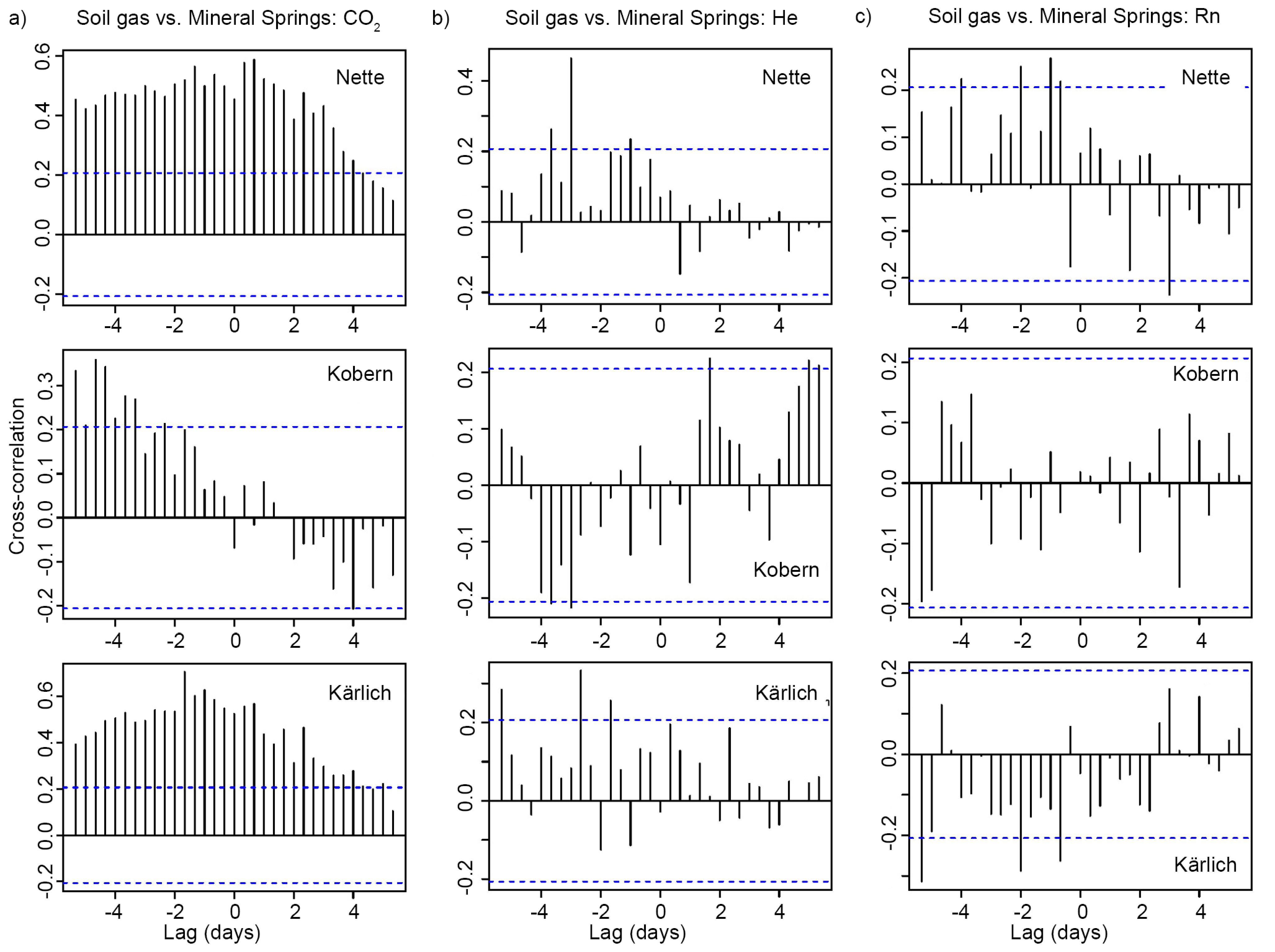
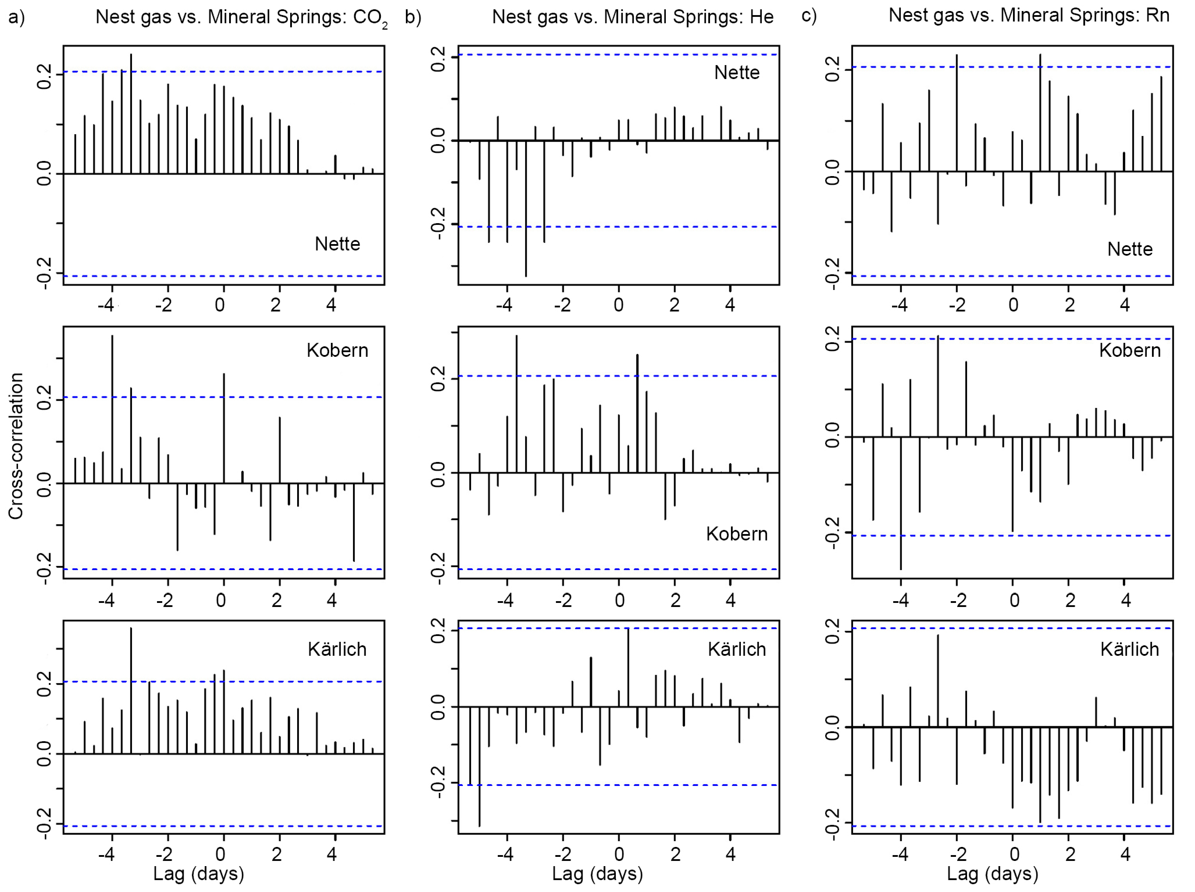
4.4. Comparison with Mineral Springs Nette, Kärlich and Kobern
5. Conclusions
Author Contributions
Funding
Acknowledgments
Conflicts of Interest
Appendix A


Appendix B


Appendix C

| Days | CO2 AA | CO2 NG | CO2 SG1 | CO2 SG2 | CO2 SG3 | CO2 SG4 | CO2 SG5 | CO2 SG6 | CO2 SG7 |
|---|---|---|---|---|---|---|---|---|---|
| 1 | |||||||||
| 2 | 0.2 | 5.0 | 5.1 | 2.7 | 0.5 | 1.3 | 1.5 | 4.2 | 1.4 |
| 3 | 0.2 | 6.2 | 7.2 | 3.5 | 0.4 | 1.6 | 1.4 | 4.1 | 2.3 |
| 4 | 0.2 | 5.1 | 9.6 | 2.5 | 0.6 | 1.6 | 1.5 | 4.1 | |
| 5 | 4.8 | 4.5 | 3.6 | 4.8 | |||||
| 6 | 0.2 | 3.9 | 9.4 | 4.2 | 0.7 | 0.7 | 1.0 | 4.1 | 4.2 |
| 7 | 11.1 | 0.5 | 1.4 | 4.0 | |||||
| 8 | 0.2 | 1.3 | 4.3 | ||||||
| 9 | 4.7 | 2.3 | |||||||
| 10 | 3.1 | 4.4 | |||||||
| 11 | 11.7 | ||||||||
| 12 | |||||||||
| 13 | 0.2 | 5.4 | 0.8 | 0.5 | 3.7 | ||||
| 14 | |||||||||
| 15 | 4.2 | ||||||||
| 16 | |||||||||
| 17 | |||||||||
| 18 | 4.2 | 1.0 | 1.3 | ||||||
| 19 | |||||||||
| 20 | |||||||||
| 21 | |||||||||
| 22 | 13.8 | 1.2 | 4.2 | ||||||
| 23 | |||||||||
| 24 | |||||||||
| 25 | |||||||||
| 26 | |||||||||
| 27 | |||||||||
| 28 | |||||||||
| 29 | |||||||||
| 30 | 2.1 | 5.0 |
| Days | He AA | He NG | He SG1 | He SG2 | He SG3 | He SG4 | He SG5 | He SG6 | He SG7 |
|---|---|---|---|---|---|---|---|---|---|
| 1 | 686.7 | 433.0 | 403.9 | 280.6 | 701.4 | 1059.3 | 307.5 | 3381.8 | 565.8 |
| 2 | 676.7 | 767.0 | 756.2 | 405.9 | 910.4 | 1370.2 | 538.6 | 4115.7 | 806.3 |
| 3 | 984.0 | 529.1 | 691.0 | 374.0 | 676.0 | 1338.3 | 638.4 | 5832.6 | 900.5 |
| 4 | 833.9 | 694.7 | 818.6 | 318.3 | 828.3 | 1073.4 | 622.2 | 6504.7 | 574.6 |
| 5 | 784.6 | 789.5 | 1.142.4 | 307.1 | 837.6 | 1252.1 | 817.8 | 622.1 | |
| 6 | 802.0 | 879.3 | 1.162.9 | 491.5 | 725.8 | 843.0 | |||
| 7 | 6.630.6 | ||||||||
| 8 | 1335.4 | 1.101.0 | |||||||
| 9 | 823.1 | 108.5 | 551.5 | 6.705.9 | |||||
| 10 | 802.5 | 983.3 | 872.1 | ||||||
| 11 | |||||||||
| 12 | 622.3 | 175.0 | 862.1 | 794.3 | 6.771.3 | ||||
| 13 | 559.6 | ||||||||
| 14 | |||||||||
| 15 | |||||||||
| 16 | |||||||||
| 17 | 624.8 | 702.5 | |||||||
| 18 | |||||||||
| 19 | |||||||||
| 20 | |||||||||
| 21 | 436.3 | 840.2 | 1267.7 | 7296.0 | 1273.0 | ||||
| 22 | |||||||||
| 23 | |||||||||
| 24 | |||||||||
| 25 | |||||||||
| 26 | |||||||||
| 27 | |||||||||
| 28 | |||||||||
| 29 | 1.421.4 | ||||||||
| 30 | 686.7 | 433.0 | 403.9 | 280.6 | 701.4 | 1.059.3 | 307.5 | 3.381.8 | 565.8 |
| … | |||||||||
| 45 | 362.3 | 2.087.6 | 1.046.9 |
| Days | Rn AA | Rn NG | Rn SG1 | Rn SG2 | Rn SG3 | Rn SG4 | Rn SG5 | Rn SG6 | Rn SG7 |
|---|---|---|---|---|---|---|---|---|---|
| 1 | 1.5 | 17.2 | 51.1 | 34.9 | 12.0 | 62.0 | 53.9 | 40.1 | 28.3 |
| 2 | 1.5 | 47.2 | 55.3 | 16.7 | 188.3 | 35.6 | 59.8 | 64.5 | |
| 3 | 2.6 | 37.4 | 164.9 | 47.3 | 10.7 | 211.8 | 95.7 | 49.1 | 75.3 |
| 4 | 1.5 | 21.9 | 143.2 | 75.6 | 13.4 | 67.7 | 109.3 | 67.3 | |
| 5 | 1.8 | 21.0 | 54.5 | 19.5 | 40.9 | 48.3 | 60.9 | ||
| 6 | 2.1 | 9.9 | 101.0 | ||||||
| 7 | 17.8 | 11.8 | |||||||
| 8 | 45.4 | 128.6 | 58.1 | ||||||
| 9 | 47.3 | 55.6 | |||||||
| 10 | 2.5 | 12.4 | 62.5 | ||||||
| 11 | |||||||||
| 12 | 77.3 | ||||||||
| 13 | 218.3 | 141.4 | 129.6 | ||||||
| 14 | 2.6 | 92.9 | |||||||
| 15 | |||||||||
| 16 | |||||||||
| 17 | 37.8 | 70.6 | 40.7 | ||||||
| 18 | |||||||||
| 19 | |||||||||
| 20 | |||||||||
| 21 | 11.2 | ||||||||
| 22 | |||||||||
| 23 | |||||||||
| 24 | |||||||||
| 25 | |||||||||
| 26 | |||||||||
| 27 | |||||||||
| 28 | |||||||||
| 29 | 0.9 | ||||||||
| 30 | 1.5 | 17.2 | 51.1 | 34.9 | 12.0 | 62.0 | 53.9 | 40.1 | 28.3 |
| … | |||||||||
| 41 | 129.6 | ||||||||
| … | |||||||||
| 45 | 58.7 | 426.5 |
Appendix D
| 7-M (bi-weekly; 01.03.–30.09.2016) (a) | 4-W (8-hrs. 12.07.–11.08.2016) (b) | ||||||||||||||
|---|---|---|---|---|---|---|---|---|---|---|---|---|---|---|---|
| N | Mean | Median | Min | Max | SD | Vol. % | N | Mean | Median | Min | Max | SD | Vol. % | ||
| Nette | He (ppm) | 16 | 47.06 | 49.74 | 17.37 | 58.17 | 10.91 | 63.63 | 79 | 49.20 | 50.29 | 20.83 | 110.40 | 13.24 | 67.55 |
| Rn (Bq/L) | 16 | 6.47 | 6.26 | 2.62 | 9.46 | 1.88 | 9.11 | 79 | 8.01 | 6.58 | 0.56 | 59.90 | 8.08 | 12.92 | |
| Kärlich | He (ppm) | 16 | 7.77 | 7.80 | 6.21 | 9.03 | 839.47 | 9.16 | 79 | 7.84 | 7.77 | 6.02 | 10.95 | 0.82 | 9.06 |
| Rn (Bq/L) | 16 | 72.44 | 73.69 | 38.32 | 114.02 | 15.22 | 92.00 | 79 | 73.73 | 78.11 | 4.91 | 92.33 | 15.58 | 99.71 | |
| Kobern | He (ppm) | 16 | 2.97 | 2.02 | 0.98 | 1.11 | 2.55 | 5.56 | 79 | 4.38 | 4.48 | 1.00 | 7.50 | 1.24 | 6.23 |
| Rn (Bq/L) | 16 | 45.78 | 46.63 | 16.90 | 64.84 | 11.41 | 62.48 | 79 | 48.66 | 49.97 | 7.82 | 79.78 | 9.67 | 61.47 | |
| NG | He (ppm) | 16 | 5.11 | 5.17 | 4.09 | 5.27 | 0.28 | 5.45 | 83 | 5.17 | 5.22 | 2.90 | 5.85 | 0.32 | 5.49 |
| Rn (Bq/L) | 16 | 1.77 | 1.63 | 0.05 | 6.06 | 1.53 | 3.90 | 83 | 5.85 | 5.09 | 0.19 | 15.65 | 4.39 | 12.57 | |
| SG1 | He (ppm) | 16 | 5.12 | 5.19 | 4.55 | 5.32 | 0.18 | 5.45 | 83 | 5.08 | 5.15 | 1.71 | 5.69 | 0.46 | 5.48 |
| Rn (Bq/L) | 16 | 86.30 | 100.49 | 11.07 | 138.33 | 33.75 | 156.46 | 83 | 64.50 | 67.03 | 0.32 | 96.81 | 17.91 | 89.25 | |
| SG2 | He (ppm) | 16 | 5.23 | 5.21 | 5.11 | 5.45 | 0.09 | 5.37 | 83 | 5.21 | 5.21 | 5.07 | 5.35 | 0.06 | 5.30 |
| Rn (Bq/L) | 16 | 19.78 | 20.74 | 5.89 | 29.68 | 6.83 | 31.81 | 83 | 12.77 | 12.56 | 0.10 | 59.79 | 6.59 | 18.97 | |
| SG3 | He (ppm) | 16 | 5.12 | 5.12 | 4.63 | 5.50 | 0.22 | 5.41 | 83 | 5.21 | 5.19 | 4.60 | 10.40 | 0.62 | 5.56 |
| Rn (Bq/L) | 16 | 2.96 | 2.64 | 0.68 | 7.17 | 1.61 | 5.04 | 83 | 3.92 | 3.40 | 0.19 | 43.66 | 4.85 | 7.13 | |
| SG4 | He (ppm) | 16 | 5.16 | 5.18 | 4.75 | 5.35 | 0.13 | 5.34 | 83 | 5.29 | 5.18 | 1.77 | 11.18 | 0.99 | 5.82 |
| Rn (Bq/L) | 16 | 113.83 | 118.00 | 53.75 | 162.90 | 33.28 | 172.76 | 83 | 92.38 | 98.58 | 23.81 | 145.71 | 26.99 | 141.84 | |
| SG5 | He (ppm) | 16 | 5.01 | 5.06 | 4.50 | 5.23 | 0.21 | 5.32 | 83 | 5.12 | 5.11 | 4.76 | 5.54 | 0.11 | 5.27 |
| Rn (Bq/L) | 16 | 74.46 | 79.87 | 40.68 | 99.79 | 16.18 | 107.16 | 83 | 55.17 | 57.28 | 12.47 | 74.91 | 12.63 | 76.41 | |
| SG6 | He (ppm) | 16 | 5.16 | 5.15 | 5.00 | 5.25 | 0.07 | 5.25 | 83 | 5.25 | 5.17 | 4.88 | 11.10 | 0.67 | 5.50 |
| Rn (Bq/L) | 16 | 8.65 | 7.87 | 2.78 | 14.31 | 3.09 | 12.67 | 83 | 11.69 | 10.63 | 0.72 | 64.55 | 8.43 | 17.48 | |
| SG7 | He (ppm) | 16 | 5.20 | 5.20 | 4.93 | 5.55 | 0.15 | 5.39 | 83 | 5.10 | 5.16 | 1.69 | 5.33 | 0.40 | 5.42 |
| Rn (Bq/L) | 16 | 48.29 | 41.04 | 0.13 | 94.42 | 27.51 | 89.05 | 83 | 32.17 | 31.17 | 0.57 | 69.08 | 12.51 | 50.26 | |
Appendix E

Appendix F

Appendix G
| N | Mean | Median | Min | Max | SD | Vol. % | ||
|---|---|---|---|---|---|---|---|---|
| (a) Laacher See pasture (24.9–27.9.2007; [9]) | ||||||||
| SG | CO2 (Vol. %) | 87 | 13.80 | 3.30 | 0.03 | 100.00 | 23.70 | n.d. |
| He (ppm) | 87 | 5.44 | 5.25 | 1.33 | 10.10 | 1.00 | n.d. | |
| Rn (BqL−1) | 70 | 8.63 | 6.96 | 0.12 | 30.80 | 6.84 | n.d. | |
| (b) Obermendig Site (24.9–27.9. 2007; [9]) | ||||||||
| SG | CO2 (Vol. %) | 12 | 14.50 | 5.30 | 0.13 | 90.00 | 24.00 | n.d. |
| He (ppm) | 12 | 4.93 | 5.16 | 2.75 | 5.26 | 0.67 | n.d. | |
| Rn (BqL−1) | 12 | 24.50 | 18.30 | 0.33 | 81.00 | 24.50 | n.d. | |
| (c) Random samplings at Goloring site (29.4.2010; Berberich. unpublished) | ||||||||
| SG | CO2 (Vol. %) | 9 | 4.18 | 2.00 | 1.20 | 13.00 | 4.39 | 8.69 |
| He (ppm) | 9 | 5.16 | 5.18 | 5.07 | 5.25 | 67.50 | 5.23 | |
| Rn (BqL−1) | 9 | 32.02 | 19.24 | 0.06 | 91.18 | 29.27 | 65.58 | |
| (d) Goloring site 7-M (bi-weekly; 01.03.–30.09.2016; this study) | ||||||||
| SGmean | CO2 (Vol. %) | 112 | 4.03 | 3.20 | 0.00 | 15.00 | 3.55 | 8.74 |
| He (ppm) | 112 | 5.14 | 5.17 | 4.50 | 5.55 | 1.67 | 5.38 | |
| Rn (BqL−1) | 112 | 50.61 | 34.46 | 0.13 | 162.90 | 44.83 | 112.85 | |
| (e) Goloring site 4-W (8-hrs; 12.07.–11.08.2016; this study) | ||||||||
| SGmean | CO2 (Vol. %) | 630 | 5.17 | 4.00 | 0.00 | 14.90 | 4.03 | 10.60 |
| He (ppm) | 83 | 5.18 | 5.17 | 1.69 | 11.18 | 5.52 | 5.45 | |
| Rn (BqL−1) | 83 | 39.03 | 29.36 | 0.10 | 145.71 | 33.64 | 87.44 | |
References
- Wörner, G. Quaternary Eifel volcanism, its mantle sources and effect on the crust of the Rhenish Shield. In Young Tectonics–Magmatism–Fluids, a Case Study of the Rhenish Massif; SFB 350: Wechselwirkungen kontinentaler Stoffsysteme und ihre Modellierung: Bonn, Germany, 1998. [Google Scholar]
- Ritter, J.R.R.; Jordan, M.; Christensen, U.; Achauer, U. A mantle plume below the Eifel volcanic fields, Germany. Earth Planet. Sci. Lett. 2001, 186, 7–14. [Google Scholar] [CrossRef]
- Schmincke, H.U. The Quaternary volcanic fields of the East and the West Eifel (Germany). In Mantle Plumes; Springer: Berlin, Germany, 2007; pp. 241–322. [Google Scholar]
- Ahorner, L. Historical seismicity and present-day microearthquake activity in the Rhenish Massif, Central Europe. In Plateau Uplift: The Rhenish Shield—A Case History; Fuchs, K., von Gehlen, K., Mälzer, H., Murawski, H., Semmel, A., Eds.; Springer: Berlin, Germany, 1983; pp. 198–221. [Google Scholar]
- Hinzen, K.G. Stress field in the Northern Rhine area, Central Europe, from earthquake fault plane solutions. Tectonophysics 2003, 377, 325–356. [Google Scholar] [CrossRef]
- May, F. Quantifizierung des CO2-Flusses zur Abbildung magmatischer Prozesse im Untergrund der Westeifel; Shaker Verlag: Aachen, Germany, 2002. [Google Scholar]
- Clauser, C.; Griesshaber, E.; Neugebauer, H.J. Decoupled thermal and mantle helium anomalies: Implications for the transport regime in continental rift zones. J. Geophys. Res. 2002, 107, 2269. [Google Scholar] [CrossRef]
- Bräuer, K.; Kämpf, H.; Niedermann, S.; Strauch, G. Indications for the existence of different magmatic reservoirs beneath the Eifel area (Germany): A multi-isotope (C, N, He, Ne, Ar) approach. Chem. Geol. 2013, 356, 193–208. [Google Scholar] [CrossRef]
- Gal, F.; Brach, M.; Braibant, G.; Jouin, F.; Michel, K. CO2 escapes in the Laacher See region, East Eifel, Germany: application of natural analogue onshore and offshore geochemical monitoring. Int. J. Greenhouse Gas. Control. 2011, 5, 1099–1118. [Google Scholar] [CrossRef]
- Baubron, J.C.; Rigo, A.; Toutain, J.P. Soil gas profiles as a tool to characterize active tectonic areas: The Jaut Pass example (Pyrenees, France). Earth Planet. Sci. Lett. 2002, 196, 69–81. [Google Scholar] [CrossRef]
- Wilkinson, M.; Gilfillan, S.M.V.; Haszeldine, R.S.; Ballentine, C.J. Plumbing the depths: Testing natural tracers of subsurface CO2 origin and migration, Utah. In Carbon Dioxide Sequestration in Geological Media–State of the Science; AAPG Studies, 2009; Volume 59, pp. 619–634. [Google Scholar]
- Ciotoli, G.; Etiope, G.; Guerra, M.; Lombardi, S. The detection of concealed faults in the Ofanto basin using the correlation between soil-gas fracture surveys. Tectonophysics 1999, 299, 321–332. [Google Scholar] [CrossRef]
- Ciotoli, G.; Lombardi, S.; Zarlenga, F. Natural leakage of helium from Italian sedimentary basins of the Adriatic structural margin. Perspectives for geological sequestration of carbon dioxide. In Advances in the Geological Storage of Carbon Dioxide; Springer Science & Business Media: Berlin, Germany, 2006; pp. 191–202. [Google Scholar]
- Etiope, G. Natural emissions of methane from geological seepage in Europe. Atmos. Environ. 2009, 43, 1430–1443. [Google Scholar] [CrossRef]
- Voltattorni, N.; Sciarra, A.; Quattrocchi, F. The Application of Soil-Gas Technique to Geothermal Exploration: Study of Hidden Potential Geothermal Systems. In Proceedings of the World Geothermal Congress, Bali, Indonesia, 25–29 April 2010; pp. 1–7. [Google Scholar]
- Birdsell, D.T.; Rajaram, H.; Dempsey, D.; Viswanathan, H.S. Hydraulic fracturing fluid migration in the subsurface: A review and expanded modeling results. Water Resour. Res. 2015, 51, 7159–7188. [Google Scholar] [CrossRef]
- Giroud, N.; Vuataz, F.D.; Schill, E. Permeable Fault Detection in Deep Geothermal Aquifer Exploration by Soil Gas Measurement. In Proceedings of the Symposium 2: Structural Geology, Tectonics and Geodynamics, Bern, Germany, 16–17 November 2012. [Google Scholar]
- Davidson, T.A.; Emerson, D.E. Direct determination of the helium 3 content of atmospheric air by mass spectrometry. J. Geophys Res. Atmosph. 1990, 95, 3565–3569. [Google Scholar] [CrossRef]
- Kockarts, G. Helium in the terrestrial atmosphere. Space Sci. Rev. 1973, 14, 723–757. [Google Scholar] [CrossRef]
- Sano, Y.; Furukawa, Y.; Takahata, N. Atmospheric helium isotope ratio: Possible temporal and spatial variations. Geochim. Cosmochim. Acta 2010, 74, 4893–4901. [Google Scholar] [CrossRef]
- Gilfillan, S.M.V.; Wilkinson, M.; Haszeldinea, R.S.; Shiptonb, Z.K.; Nelsonc, S.T.; Poredad, R.J. He and Ne as tracers of natural CO2 migration up a fault from a deep reservoir. Int. J. Greenhouse Gas. Control. 2011, 5, 1507–1516. [Google Scholar] [CrossRef]
- Ciotoli, G.; Lombardi, S.; Morandi, S.; Zarlenga, F. A multidisciplinary statistical approach to study the relationships between helium leakage and neo-tectonic activity in a gas province: The Vasto Basin, Abruzzo-Molise (Central Italy). AAPG Bull 2004, 88, 355–372. [Google Scholar] [CrossRef]
- Crockett, R.G.M.; Gillmore, G.K.; Phillips, P.S.; Denman, A.R.; Groves-Kirkby, C.J. Tidal synchronicity of built-environment radon levels in the UK. Geophys. Res. Let. 2006. [Google Scholar] [CrossRef]
- Berberich, G. Identifikation Junger Gasführender Störungszonen in der West–und Hocheifel Mit Hilfe von Bioindikatoren. Ph.D. Thesis, University of Duisburg-Essen, Duisburg, Germany, 2010. [Google Scholar]
- Berberich, G.; Schreiber, U. GeoBioScience: Red Wood Ants as Bioindicators for Active Tectonic Fault Systems in the West Eifel (Germany). Animals 2013, 3, 475–498. [Google Scholar] [CrossRef] [PubMed]
- Berberich, G.; Berberich, M.; Grumpe, A.; Wöhler, C.; Schreiber, U. First Results of 2.5 Year Monitoring of Red Wood Ants’ Behavioural Changes and Their Possible Correlation with Earthquake Events. Animals 2013, 3, 63–84. [Google Scholar] [CrossRef] [PubMed]
- Berberich, G.; Grumpe, A.; Berberich, M.; Klimetzek, D.; Wöhler, C. Are red wood ants (Formica rufa-group) tectonic indicators? A statistical approach. Ecol. Ind. 2016, 61, 968–979. [Google Scholar] [CrossRef]
- Berberich, G.M.; Ellison, A.M.; Berberich, M.B.; Grumpe, A.; Becker, A.; Wöhler, C. Can a Red Wood-Ant Nest Be Associated with Fault-Related CH4 Micro-Seepage? A Case Study from Continuous Short-Term In-Situ Sampling. Animals 2018, 8, 46. [Google Scholar] [CrossRef] [PubMed]
- Del Toro, I.; Berberich, G.M.; Ribbons, R.R.; Berberich, M.B.; Sanders, N.J.; Ellison, A.M. Nests of red wood ants (Formica rufa-group) are positively associated with tectonic faults: A double-blind test. PeerJ 2017, 5, e3903. [Google Scholar] [CrossRef] [PubMed]
- Risch, A.C.; Jurgensen, M.F.; Schütz, M.; Page-Dumroese, D.S. The contribution of red wood ants to soil C and N pools and CO2 emissions in subalpine forests. Ecology 2005, 86, 419–430. [Google Scholar] [CrossRef]
- Risch, A.C.; Schütz, M.; Jurgensen, M.F.; Domisch, T.; Ohashi, M.; Finér, L. CO2 emissions from red wood ant (Formica rufa group) mounds: Seasonal and diurnal patterns related to air temperature. Ann. Zool. Fennici 2005, 42, 283–290. [Google Scholar]
- Ohashi, M.; Finér, L.; Domisch, T.; Risch, A.C.; Jurgensen, M.F. CO2 efflux from a red wood ant mound in a boreal forest. Agric. For. Meteorol. 2005, 30, 131–136. [Google Scholar] [CrossRef]
- Ohashi, M.; Finér, L.; Domisch, T.; Risch, A.C.; Jurgensen, M.F.; Niemelä, P. Seasonal and diurnal CO2 efflux from red wood ant (Formica aquilonia) mounds in boreal coniferous forests. Soil Biol. Biochem. 2007, 39, 1504–1511. [Google Scholar] [CrossRef]
- Wu, H.; Lu, X.; Wu, D.; Song, L.; Yan, X.; Liu, J. Ant mounds alter spatial and temporal patterns of CO2, CH4 and N2O emissions from a marsh soil. Soil Biol. Biochem. 2013, 57, 884–891. [Google Scholar] [CrossRef]
- Berberich, G.M.; Berberich, M.B.; Ellison, A.M. Fluctuations of gas concentrations in three mineral springs of the East Eifel Volcanic field (EEVF). arXiv, 2017; arXiv:1710.04128. [Google Scholar]
- Chester, F.M.; Evans, J.P.; Biegel, R.L. Internal Structure and Weakening Mechanisms of the San Andreas Fault. J. Geophys. Res. 1993, 98, 771–786. [Google Scholar] [CrossRef]
- BNS–Erdbebenstation Bensberg. Available online: www.seismo.uni-koeln.de/catalog/index.htm (accessed on 1 September 2016).
- Reimann, C.; Filzmoser, P.; Garrett, R.G. Background and threshold: Critical comparison of methods of determination. Sci. Total Environ. 2005, 346, 1–16. [Google Scholar] [CrossRef] [PubMed]
- Hinkle, D.E.; Wiersma, W.; Jurs, S.G. Applied Statistics for the Behavioral Sciences, 5th ed.; Wadsworth Publishing: Belmont, CA, USA, 2009. [Google Scholar]
- Milbert, D. Solid Earth Tide. Version 15.02.2016. 2016. Available online: http://geodesyworld.github.io/SOFTS/solid.htm (accessed on 15 February 2016).
- Oppenheim, A.V.; Schafer, R.W.; Buck, J.R. Discrete-Time Signal Processing; Pearson Education India: Upper Saddle River, NJ, USA, 1999; pp. 468–471. [Google Scholar]
- Sauer, U.; Watanabe, N.; Singh, A.; Dietrich, P.; Kolditz, O.; Schütze, C. Joint interpretation of geoelectrical and soil-gas measurements for monitoring CO2 releases at a natural analogue. Near Surface Geophys. 2014, 12, 165–178. [Google Scholar] [CrossRef]
- Kemski, J.; Siehl, A.; Stegmann, R.; Valdivia-Manchego, M. Geogene Faktoren der Strahlenexposition unter besonderer Berücksichtigung des Radonpotentials. In Schriftenreihe Reaktorsicherheit und Naturschutz; BMU-1999-534: Bonn, Germany; p. 133.
- LGB-RLP (2017) Radonpotentialkarte der Osteifel. Landesamt für Geologie und Bergbau Rheinland-Pfalz, Ausdruck vom. Available online: http://www.lgb-rlp.de/karten-und-produkte/online-karten/online-karte-radonprognose.html. (accessed on 1 August 2017).
- Hinkle, M.E. Environmental conditions affecting concentrations of He, CO2, O2, and N2 in soil gases. Appl. Geochem. 1994, 9, 53–63. [Google Scholar] [CrossRef]
- Pfanz, H. Mofetten. In Kalter Atem schlafender Vulkane; Deutsche Vulkanologische Gesellschaft: Mendig, Germany, 2008; p. 85. [Google Scholar]
- Etiope, G.; Guerra, M.; Raschi, A. Carbon Dioxide and Radon Geohazards Over a Gas-bearing Fault in the Siena Graben (Central Italy). TAO 2005, 16, 885–896. [Google Scholar] [CrossRef]
- Risdianto, D.; Kusnadi, D. The Application of a Probability Graph in Geothermal Exploration. In Proceedings of the World Geothermal Congress 2010, Bali, Indonesia, 25–29 April 2010; pp. 1–6. [Google Scholar]
- Boothroyd, I.M.; Almond, S.; Worrall, F.; Davies, R.J. Assessing the fugitive emission of CH4 via migration along fault zones—Comparing potential shale gas basins to non-shale basins in the UK. STOTEN 2017, 580, 412–424. [Google Scholar]
- Jolie, E.; Klinkmueller, M.; Moeck, I. Diffuse Degassing Measurements in Geothermal Exploration of Fault Controlled Systems. In Proceedings of the World Geothermal Congress 2015, Melbourne, Australia, 19–25 April 2015. [Google Scholar]
- Richon, P.; Perrier, F.; Jean, E.-P.; Sabroux, C. Detectability and significance of 12 hr barometric tide in radon-222 signal, dripwater flow rate, air temperature and carbon dioxide concentration in an underground tunnel. Geophys. J. Int. 2009, 176, 3. [Google Scholar] [CrossRef]
- Kemski, J.; Klingel, R.; Siehl, A.; Neznal, M.; Matolin, N. Erarbeitung fachlicher Grundlagen zur Beurteilung der Vergleichbarkeit unterschiedlicher Messmethoden zur Bestimmung der Radonbodenluftkonzentration - Vorhaben 3609S10003. Bd. 2 Sachstandsbericht “Radonmessungen in der Bodenluft -Einflussfaktoren, Messverfahren, Bewertung”, 2012. Available online: https://doris.bfs.de/jspui/bitstream/urn:nbn:de:0221-201203237830/3/BfS_2012_3609S10003_Bd2.pdf (accessed on 18 August 2017).
- LGB RLP. Geologie von Rheinland-Pfalz; Schweizbart’sche Verlagsbuchhandlung (Nägele u. Obermiller): Stuttgart, Germany, 2005; pp. 1–400. [Google Scholar]
- Griesshaber, E. The distribution pattern of mantle derived volatiles in mineral waters of the Rhenish Massif. In Young Tectonics–Magmatism–Fluids, a Case Study of the Rhenish Massif; SFB 350: Wechselwirkungen kontinentaler Stoffsysteme und ihre Modellierung: Bonn, Germany, 1998. [Google Scholar]
- Toutain, J.P.; Baubron, J.C. Gas geochemistry and seismotectonics: A review. Tectonophysics 1999, 304, 1–27. [Google Scholar] [CrossRef]
- Padilla, G.D.; Hernández, P.A.; Padrón, E.; Barrancos, J.; Pérez, N.M.; Melián, G.; Nolasco, D.; Dionis, S.; Rodríguez, F.; Calvo, D.; et al. Soil gas radon emissions and volcanic activity at El Hierro (Canary Islands): The 2011-2012 submarine eruption, Geochem. Geophys. Geosyst. 2013, 14, 432–447. [Google Scholar] [CrossRef]
- Beaubien, S.; Jones, D.; Gal, F.; Barkwith, A.; Braibant, G.; Baubron, J.C.; Ciotoli, G.; Graziani, S.; Lister, T.; Lombardi, S. Monitoring of near-surface gasgeochemistry at the Weyburn, Canada, CO2-EOR site, 2001–2011. Int. J. Greenh. Gas. Control. 2013, 16, 236–262. [Google Scholar] [CrossRef]
- Barnet, I.; Procházka, J.; Skalský, L. Do the Earth tides have an influence on short-term variations in radon concentration? Rad. Prot. Dos. 1997, 69, 51–60. [Google Scholar] [CrossRef]


| 7-M (bi-weekly; 01.03.–30.09.2016) (a) | 4-W (8-hrs. 12.07.–11.08.2016) (b) | ||||||||||||||
|---|---|---|---|---|---|---|---|---|---|---|---|---|---|---|---|
| N | Mean | Median | Min | Max | SD | Vol. % | N | Mean | Median | Min | Max | SD | Vol. % | ||
| AA | CO2 (Vol. %) | 16 | 0.00 | 0.00 | 0.00 | 0.00 | 0.00 | 0.00 | 83 | 0.01 | 0.00 | 0.00 | 0.90 | 0.10 | 0.05 |
| He (ppm) | 16 | 5.18 | 5.20 | 5.03 | 5.32 | 0.09 | 5.33 | 83 | 5.16 | 5.24 | 1.79 | 5.54 | 0.47 | 5.55 | |
| Rn (BqL−1) | 16 | 0.31 | 0.11 | 0.00 | 3.07 | 0.74 | 0.80 | 83 | 0.43 | 0.35 | 0.05 | 1.64 | 0.29 | 0.79 | |
| NG | CO2 (Vol. %) | 16 | 0.20 | 0.00 | 0.00 | 0.80 | 0.30 | 0.50 | 83 | 0.64 | 0.40 | 0.00 | 10.80 | 1.56 | 1.58 |
| He (ppm) | 16 | 5.11 | 5.17 | 4.09 | 5.27 | 0.28 | 5.45 | 83 | 5.17 | 5.22 | 2.90 | 5.85 | 0.32 | 5.49 | |
| Rn (BqL−1) | 16 | 1.77 | 1.63 | 0.05 | 6.06 | 1.53 | 3.90 | 83 | 5.85 | 5.09 | 0.19 | 15.65 | 4.39 | 12.57 | |
| SG 1 | CO2 (Vol. %) | 16 | 5.97 | 5.30 | 3.20 | 10.40 | 2.27 | 8.94 | 83 | 8.76 | 8.80 | 3.60 | 11.00 | 1.51 | 11.06 |
| He (ppm) | 16 | 5.12 | 5.19 | 4.55 | 5.32 | 0.18 | 5.45 | 83 | 5.08 | 5.15 | 1.71 | 5.69 | 0.46 | 5.48 | |
| Rn (BqL−1) | 16 | 86.30 | 100.49 | 11.07 | 138.33 | 33.75 | 156.46 | 83 | 64.50 | 67.03 | 0.32 | 96.81 | 17.91 | 89.25 | |
| SG 2 | CO2 (Vol. %) | 16 | 3.58 | 3.20 | 0.60 | 6.60 | 1.72 | 5.79 | 83 | 4.06 | 4.20 | 0.80 | 5.80 | 0.88 | 5.29 |
| He (ppm) | 16 | 5.23 | 5.21 | 5.11 | 5.45 | 0.09 | 5.37 | 83 | 5.21 | 5.21 | 5.07 | 5.35 | 0.06 | 5.30 | |
| Rn (BqL−1) | 16 | 19.78 | 20.74 | 5.89 | 29.68 | 6.83 | 31.81 | 83 | 12.77 | 12.56 | 0.10 | 59.79 | 6.59 | 18.97 | |
| SG 3 | CO2 (Vol. %) | 16 | 0.90 | 0.40 | 0.00 | 6.00 | 1.56 | 2.23 | 83 | 1.12 | 1.20 | 0.00 | 1.60 | 0.18 | 1.45 |
| He (ppm) | 16 | 5.12 | 5.12 | 4.63 | 5.50 | 0.22 | 5.41 | 83 | 5.21 | 5.19 | 4.60 | 10.40 | 0.62 | 5.56 | |
| Rn (BqL−1) | 16 | 2.96 | 2.64 | 0.68 | 7.17 | 1.61 | 5.04 | 83 | 3.92 | 3.40 | 0.19 | 43.66 | 4.85 | 7.13 | |
| SG 4 | CO2 (Vol. %) | 16 | 2.50 | 2.40 | 0.60 | 4.20 | 1.13 | 4.33 | 83 | 3.70 | 3.80 | 1.40 | 4.40 | 0.48 | 4.42 |
| He (ppm) | 16 | 5.16 | 5.18 | 4.75 | 5.35 | 0.13 | 5.34 | 83 | 5.29 | 5.18 | 1.77 | 11.18 | 0.99 | 5.82 | |
| Rn (BqL−1) | 16 | 113.83 | 118.00 | 53.75 | 162.90 | 33.28 | 172.76 | 83 | 92.38 | 98.58 | 23.81 | 145.71 | 26.99 | 141.84 | |
| SG 5 | CO2 (Vol. %) | 16 | 10.39 | 10.00 | 6.40 | 15.00 | 2.48 | 14.00 | 83 | 12.77 | 12.50 | 3.60 | 14.90 | 1.30 | 13.89 |
| He (ppm) | 16 | 5.01 | 5.06 | 4.50 | 5.23 | 0.21 | 5.32 | 83 | 5.12 | 5.11 | 4.76 | 5.54 | 0.11 | 5.27 | |
| Rn (BqL−1) | 16 | 74.46 | 79.87 | 40.68 | 99.79 | 16.18 | 107.16 | 83 | 55.17 | 57.28 | 12.47 | 74.91 | 12.63 | 76.41 | |
| SG 6 | CO2 (Vol. %) | 16 | 0.75 | 0.60 | 0.00 | 1.80 | 0.51 | 1.39 | 83 | 1.05 | 1.00 | 0.00 | 1.40 | 0.24 | 1.36 |
| He (ppm) | 16 | 5.16 | 5.15 | 5.00 | 5.25 | 0.07 | 5.25 | 83 | 5.25 | 5.17 | 4.88 | 11.10 | 0.67 | 5.50 | |
| Rn (BqL−1) | 16 | 8.65 | 7.87 | 2.78 | 14.31 | 3.09 | 12.67 | 83 | 11.69 | 10.63 | 0.72 | 64.55 | 8.43 | 17.48 | |
| SG 7 | CO2 (Vol. %) | 16 | 3.95 | 3.80 | 1.80 | 6.60 | 1.46 | 6.14 | 83 | 4.61 | 4.60 | 3.20 | 6.40 | 0.91 | 6.12 |
| He (ppm) | 16 | 5.20 | 5.20 | 4.93 | 5.55 | 0.15 | 5.39 | 83 | 5.10 | 5.16 | 1.69 | 5.33 | 0.40 | 5.42 | |
| Rn (BqL−1) | 16 | 48.29 | 41.04 | 0.13 | 94.42 | 27.51 | 89.05 | 83 | 32.17 | 31.17 | 0.57 | 69.08 | 12.51 | 50.26 | |
| Classes | AA | NG | SG1 | SG2 | SG3 | SG4 | SG5 | SG6 | SG7 |
|---|---|---|---|---|---|---|---|---|---|
| (a) CO2 (Vol. %) 1 | |||||||||
| I: <1 | 100.0 | 96.4 | 0.0 | 0.0 | 2.4 | 0.0 | 0.0 | 1.2 | 0.0 |
| II: 1–9.99 | 0.0 | 2.4 | 74.7 | 100 | 97.6 | 100 | 1.2 | 97.6 | 100 |
| III: >10 | 0.0 | 1.2 | 25.3 | 0.0 | 0.0 | 0.0 | 98.8 | 1.2 | 0.0 |
| Sum (%) | 100.0 | 100.0 | 100.0 | 100.0 | 100.0 | 100.0 | 100.0 | 100.0 | 100.0 |
| (b) He (ppm) | |||||||||
| I: <5.22 2 (undisturbed background levels) | 39.8 | 50.6 | 84.3 | 60.2 | 59.0 | 77.1 | 85.5 | 80.7 | 86.7 |
| II: 5.22–5.29 | 48.2 | 38.6 | 12.0 | 33.8 | 30.1 | 14.5 | 10.8 | 15.7 | 12.0 |
| III: 5.30–5.39 | 9.6 | 7.2 | 1.2 | 6.0 | 9.6 | 2.4 | 1.2 | 1.2 | 1.3 |
| IV: 5.40–5.59 | 2.4 | 2.4 | 1.2 | 0.0 | 0.0 | 2.4 | 2.5 | 0.0 | 0.0 |
| V: >5.60 | 0.0 | 1.2 | 1.3 | 0.0 | 1.3 | 3.6 | 0.0 | 2.4 | 0.0 |
| Sum (%) | 100.0 | 100.0 | 100.0 | 100.0 | 100.0 | 100.0 | 100.0 | 100.0 | 100.0 |
| Sum (%) >5.22 ppm | 60.2 | 49.4 | 15.7 | 39.8 | 41.0 | 22.9 | 14.5 | 19.3 | 13.3 |
| (c) Rn (BqL−1) | |||||||||
| I: <20 (background concentration) 3 | 100 | 100 | 3.6 | 98.8 | 98.8 | 0.0 | 1.2 | 96.3 | 15.7 |
| II: 20–39.9 (low-moderate) 3 | 0.0 | 0.0 | 3.6 | 0.0 | 0.0 | 4.8 | 9.6 | 0.0 | 57.8 |
| III: 40–99.9 (increased with locally high potential > 100 BqL−1) 3 | 0.0 | 0.0 | 92.8 | 1.2 | 1.2 | 49.3 | 89.2 | 3.7 | 26.5 |
| IV: >100 (locally high potential) 4 | 0.0 | 0.0 | 0.0 | 0.0 | 0.0 | 45.9 | 0.0 | 0.0 | 0.0 |
| Sum (%) | 100.0 | 100.0 | 100.0 | 100.0 | 100.0 | 100.0 | 100.0 | 100.0 | 100.0 |
© 2018 by the authors. Licensee MDPI, Basel, Switzerland. This article is an open access article distributed under the terms and conditions of the Creative Commons Attribution (CC BY) license (http://creativecommons.org/licenses/by/4.0/).
Share and Cite
Berberich, G.M.; Berberich, M.B.; Ellison, A.M.; Wöhler, C. Degassing Rhythms and Fluctuations of Geogenic Gases in A Red Wood-Ant Nest and in Soil in The Neuwied Basin (East Eifel Volcanic Field, Germany). Insects 2018, 9, 135. https://doi.org/10.3390/insects9040135
Berberich GM, Berberich MB, Ellison AM, Wöhler C. Degassing Rhythms and Fluctuations of Geogenic Gases in A Red Wood-Ant Nest and in Soil in The Neuwied Basin (East Eifel Volcanic Field, Germany). Insects. 2018; 9(4):135. https://doi.org/10.3390/insects9040135
Chicago/Turabian StyleBerberich, Gabriele M., Martin B. Berberich, Aaron M. Ellison, and Christian Wöhler. 2018. "Degassing Rhythms and Fluctuations of Geogenic Gases in A Red Wood-Ant Nest and in Soil in The Neuwied Basin (East Eifel Volcanic Field, Germany)" Insects 9, no. 4: 135. https://doi.org/10.3390/insects9040135
APA StyleBerberich, G. M., Berberich, M. B., Ellison, A. M., & Wöhler, C. (2018). Degassing Rhythms and Fluctuations of Geogenic Gases in A Red Wood-Ant Nest and in Soil in The Neuwied Basin (East Eifel Volcanic Field, Germany). Insects, 9(4), 135. https://doi.org/10.3390/insects9040135