Author Contributions
Conceptualization, Y.W., C.L., C.J. and M.D.; data curation, M.L.; formal analysis, B.Y.; funding acquisition, M.D.; investigation, S.X.; methodology, Y.W., C.L. and C.J.; project administration, M.D.; resources, M.L.; software, Y.W., C.L., C.J. and S.X.; supervision, M.D.; validation, S.X. and B.Y.; visualization, M.L. and B.Y.; writing—original draft, Y.W., C.L., C.J., M.L., S.X., B.Y. and M.D.; Y.W., C.L., C.J. and M.L. contributed equally to this work. All authors have read and agreed to the published version of the manuscript.
Figure 1.
Examples of image augmentation methods that destroy the fragile semantics of agricultural images.
Figure 1.
Examples of image augmentation methods that destroy the fragile semantics of agricultural images.
Figure 2.
Overview of CropCLR-Wheat framework. A two-stage pipeline integrating unsupervised contrastive pretraining, lightweight fine-tuning with attention, and deployment on edge and mobile platforms for robust wheat pest recognition.
Figure 2.
Overview of CropCLR-Wheat framework. A two-stage pipeline integrating unsupervised contrastive pretraining, lightweight fine-tuning with attention, and deployment on edge and mobile platforms for robust wheat pest recognition.
Figure 3.
Example images of wheat pest categories, including Sitodiplosis mosellana (a), Tetranychus cinnbarinus (b), Dolerus tritici Chu (c), Mythimna separata (d), Anguina tritici (e), Gryllotalpa orientalis (f), and Elateridae (g).
Figure 3.
Example images of wheat pest categories, including Sitodiplosis mosellana (a), Tetranychus cinnbarinus (b), Dolerus tritici Chu (c), Mythimna separata (d), Anguina tritici (e), Gryllotalpa orientalis (f), and Elateridae (g).
Figure 4.
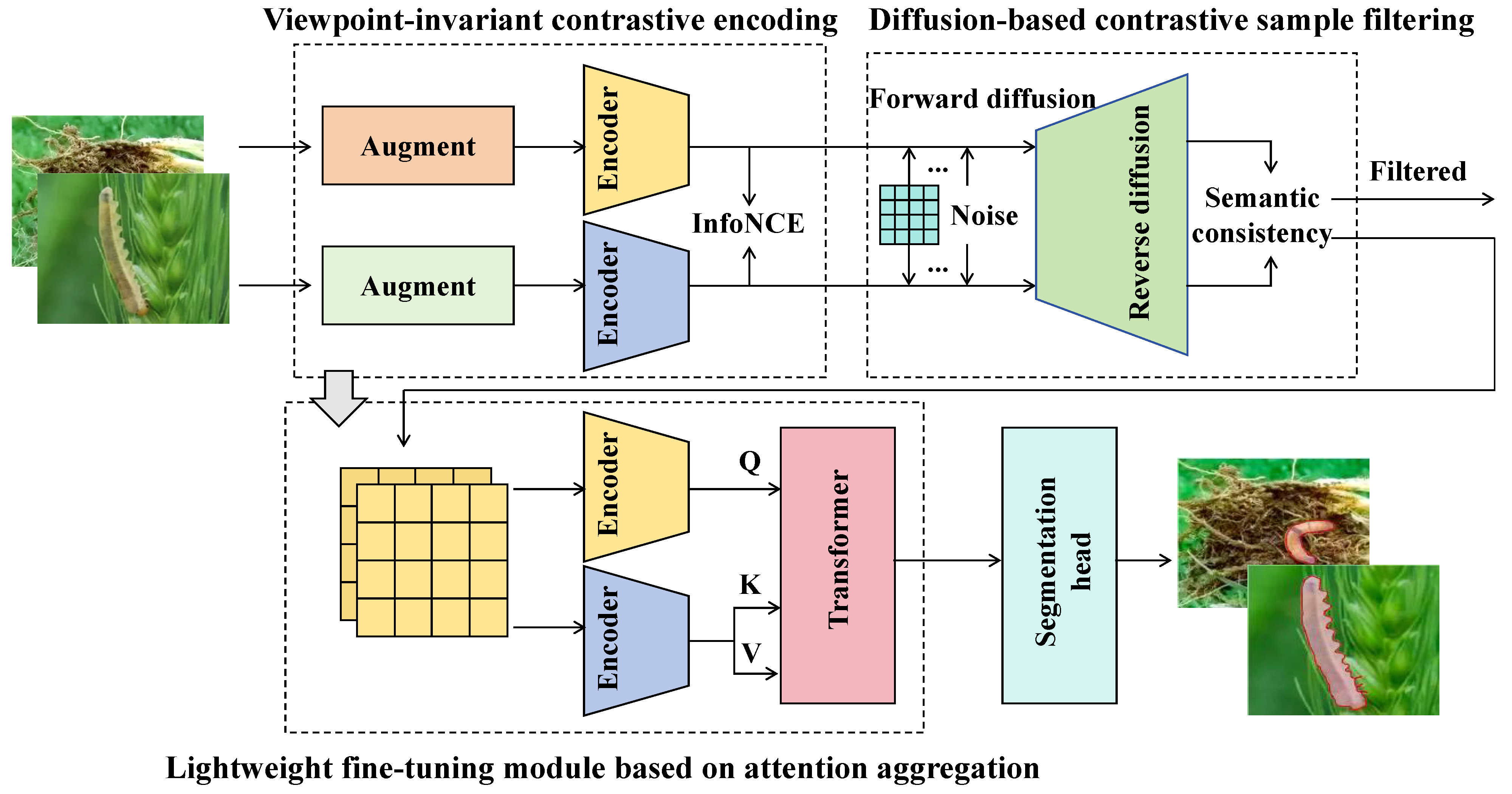
Schematic diagram of the overall architecture of CropCLR-Wheat.
Figure 4.
Schematic diagram of the overall architecture of CropCLR-Wheat.
Figure 5.
This diagram illustrates the structure of the viewpoint-invariant contrastive encoding module designed to address pose and viewpoint variations in field imagery. The input image is processed by a shared encoder, whose weights are updated via exponential moving average (EMA) to produce a momentum encoder. Positive and negative samples are fed into the momentum encoder and projected via MLP for contrastive alignment. The encoder output is simultaneously decoded to yield segmentation or detection predictions, supervised by a BCEDice loss for segmentation or a combination of Smooth L1 Loss and cross-entropy loss terms for detection.
Figure 6.
This figure illustrates the architecture of the diffusion-based contrastive sample filtering module, which addresses sample heterogeneity in agricultural pest recognition. The module consists of a forward diffusion process that progressively adds Gaussian noise to the encoded feature map and a reverse reconstruction process implemented via a conditional variational autoencoder with four transformer layers. The reverse process outputs two decoder branches, and , representing the mean and variance for semantic reconstruction. The two input feature maps correspond to distinct augmented views and , which are compared after reconstruction to evaluate semantic consistency and filter out inconsistent samples.
Figure 7.
Lightweight fine-tuning module based on attention aggregation. This figure illustrates a lightweight fine-tuning framework that addresses label scarcity in wheat pest recognition tasks. The framework begins with a linear projection, followed by embedding generation from classification, image, and register tokens. The ViT encoder, composed of stacked multi-head attention and feed-forward layers, processes these embeddings. During training, an attention head pruning strategy is applied to remove redundant or less informative attention heads, and classification is conducted using masked token prediction through a linear layer. During inference, only the most discriminative attention maps are retained, significantly reducing computational cost while preserving classification accuracy.
Figure 8.
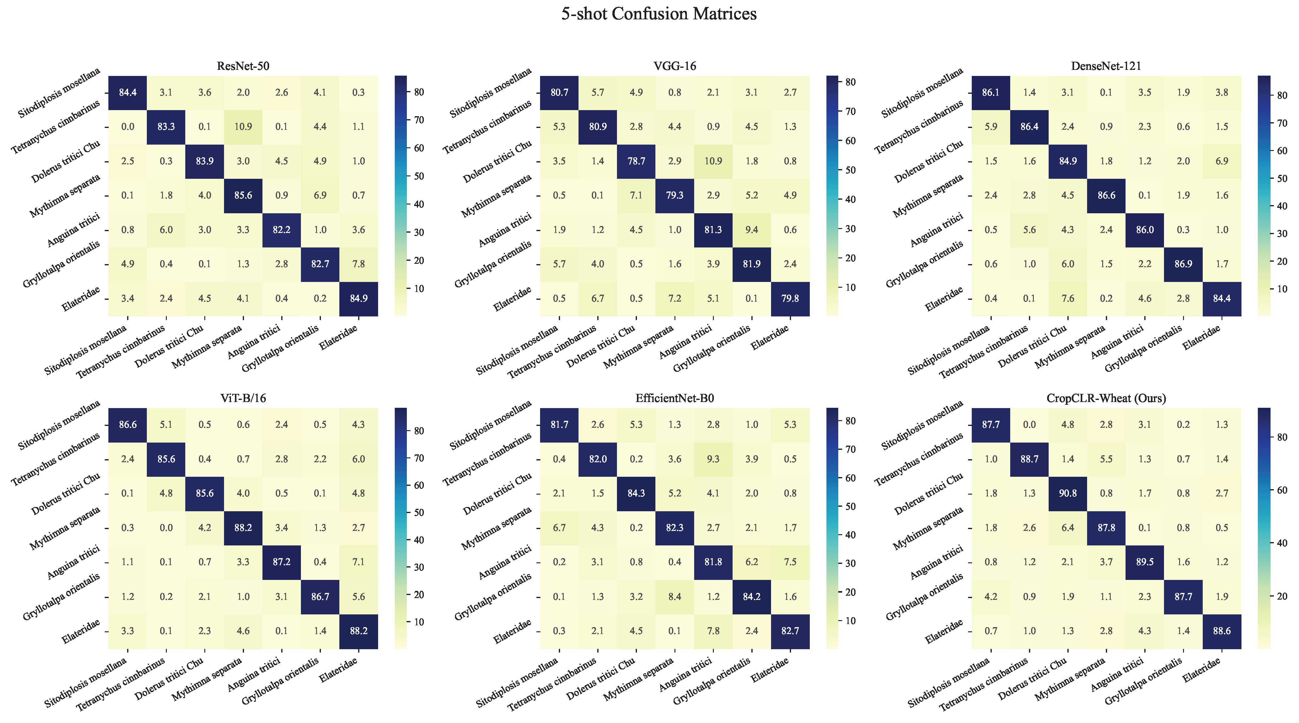
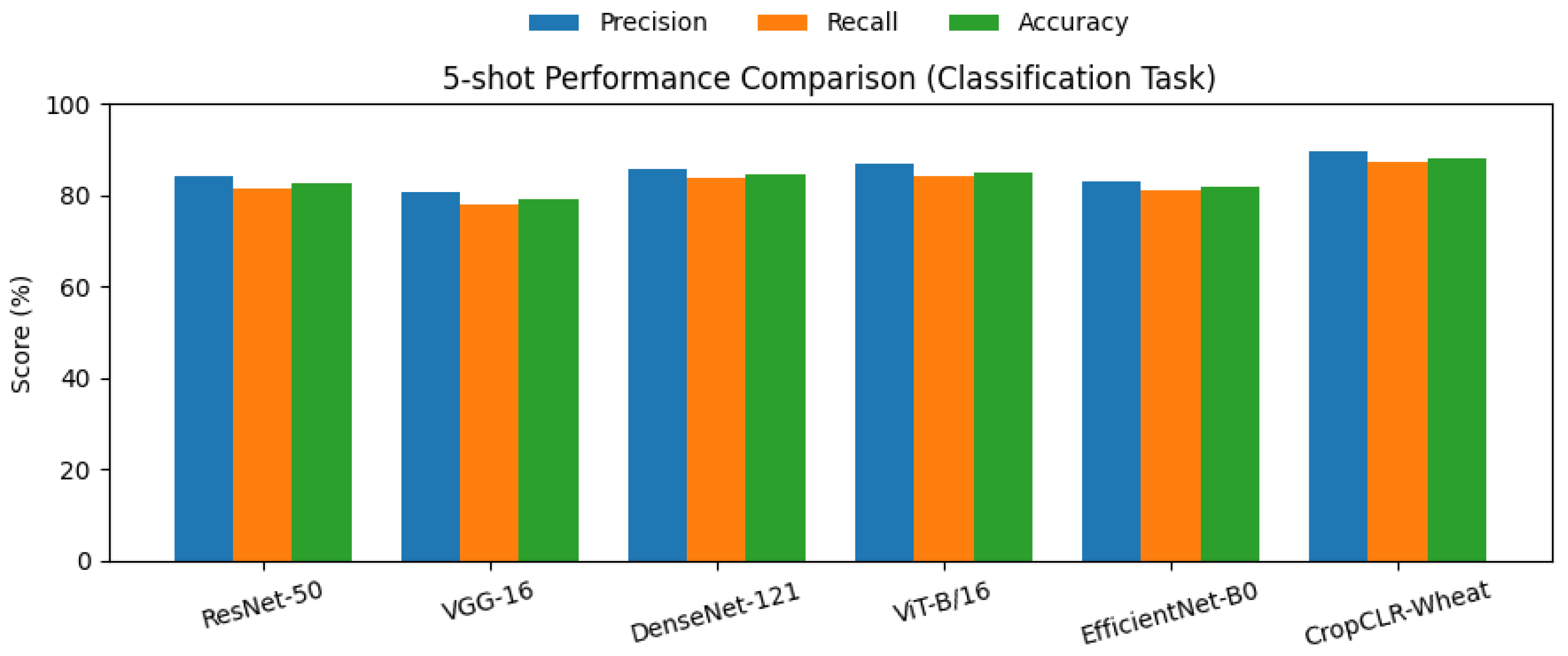
This bar chart illustrates the performance comparison of six models—ResNet-50, VGG-16, DenseNet-121, ViT-B/16, EfficientNet-B0, and the proposed CropCLR-Wheat—on the 5-shot wheat pest classification task.
Figure 8.
This bar chart illustrates the performance comparison of six models—ResNet-50, VGG-16, DenseNet-121, ViT-B/16, EfficientNet-B0, and the proposed CropCLR-Wheat—on the 5-shot wheat pest classification task.
Figure 9.
This bar chart presents the classification performance of six models—ResNet-50, VGG-16, DenseNet-121, ViT-B/16, EfficientNet-B0, and CropCLR-Wheat—on the 10-shot wheat pest classification task.
Figure 9.
This bar chart presents the classification performance of six models—ResNet-50, VGG-16, DenseNet-121, ViT-B/16, EfficientNet-B0, and CropCLR-Wheat—on the 10-shot wheat pest classification task.
Figure 10.
Performance comparison of different models on the wheat ear detection task. This line chart presents the evaluation results of baseline models on the wheat ear detection task.
Figure 10.
Performance comparison of different models on the wheat ear detection task. This line chart presents the evaluation results of baseline models on the wheat ear detection task.
Figure 11.
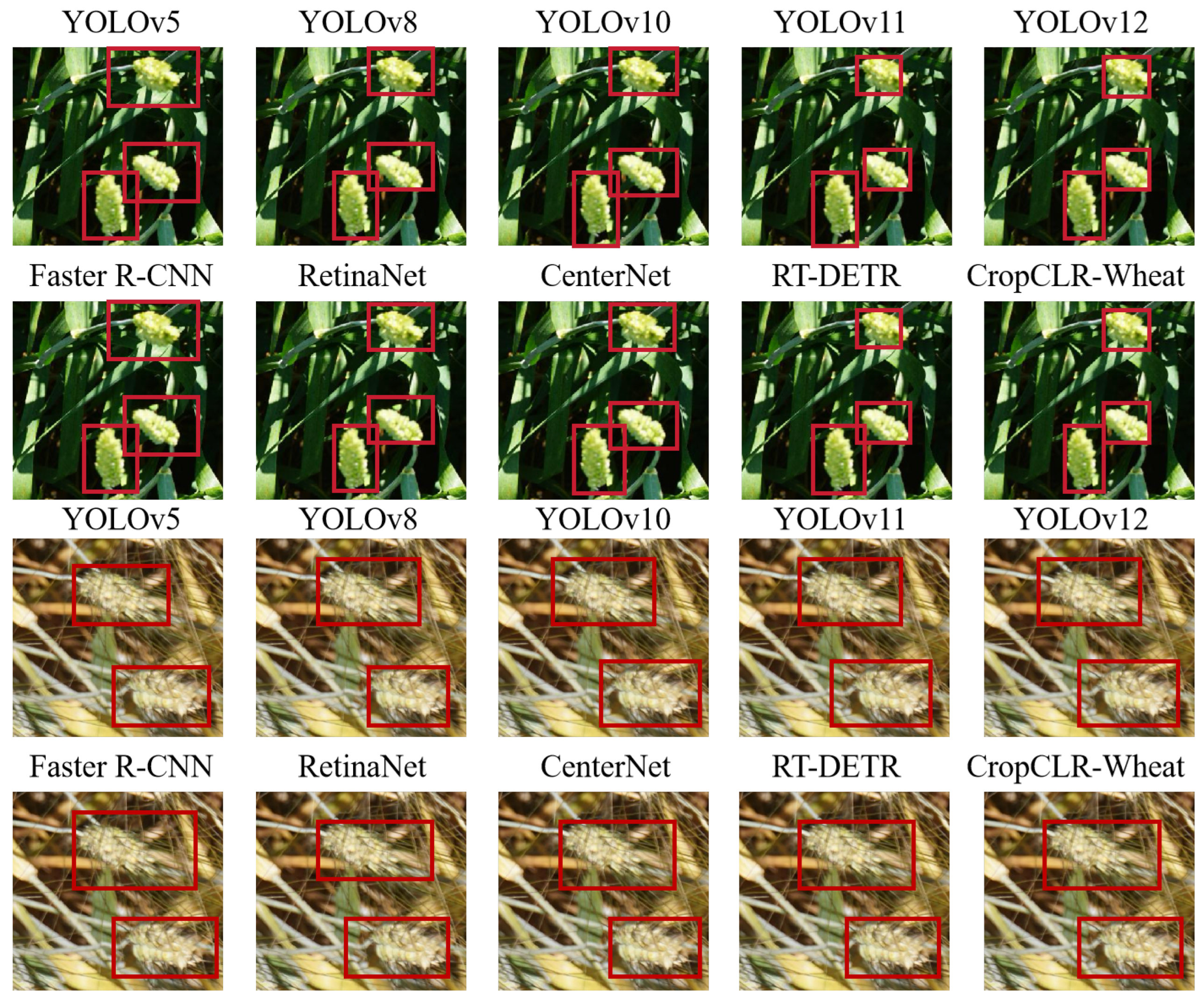
Detection results of different models.
Figure 11.
Detection results of different models.
Figure 12.
Segmentation of different models.
Figure 12.
Segmentation of different models.
Figure 13.
Radar chart comparison of segmentation performance on wheat pest damage data. This radar chart illustrates the segmentation performance of six models—UNet, DeepLabV3+, PSPNet, Segformer, Mask R-CNN, and CropCLR-Wheat—across three key metrics: precision, recall, and accuracy.
Figure 13.
Radar chart comparison of segmentation performance on wheat pest damage data. This radar chart illustrates the segmentation performance of six models—UNet, DeepLabV3+, PSPNet, Segformer, Mask R-CNN, and CropCLR-Wheat—across three key metrics: precision, recall, and accuracy.
Figure 14.
Prediction consistency of different models under visual distortions. This line chart evaluates the robustness of five models—ResNet-50, SimCLR, MoCo-v2, ViT-B/16, and CropCLR-Wheat—under increasing levels of visual distortion, measured by rotation angles from 0° to 50°.
Figure 14.
Prediction consistency of different models under visual distortions. This line chart evaluates the robustness of five models—ResNet-50, SimCLR, MoCo-v2, ViT-B/16, and CropCLR-Wheat—under increasing levels of visual distortion, measured by rotation angles from 0° to 50°.
Figure 15.
Module ablation study under 5-shot and 10-shot settings. This bar chart presents the performance impact of different modules in the CropCLR-Wheat framework, evaluated under both 5-shot and 10-shot learning scenarios.
Figure 15.
Module ablation study under 5-shot and 10-shot settings. This bar chart presents the performance impact of different modules in the CropCLR-Wheat framework, evaluated under both 5-shot and 10-shot learning scenarios.
Table 1.
Image sources and quantities for the CropField-U dataset.
Table 1.
Image sources and quantities for the CropField-U dataset.
| Source | Location | Device | Image Count |
|---|
| Field capture (pest) | Yutian, Tangshan | Phantom 4/iPhone 13 Pro | 8200 |
| Field capture (pest) | Wuyuan, Bayannur | Phantom 4/RICOH G900 | 6400 |
| Irrigation/post-harvest (control) | Mixed locations | Phantom 4/iPhone 13 Pro | 3000 |
| PlantVillage (wheat) | Online open-source | - | 3200 |
| AI Challenger/Web sources | Multiple regions | - | 3800 |
| Total | - | - | 24,600 |
Table 2.
Performance comparison of different models on wheat pest classification under 5-shot and 10-shot fine-tuning (mean ± std over 3 runs). Bold results are significantly better than ResNet-50 baseline (** p < 0.01).
Table 2.
Performance comparison of different models on wheat pest classification under 5-shot and 10-shot fine-tuning (mean ± std over 3 runs). Bold results are significantly better than ResNet-50 baseline (** p < 0.01).
| Model | 5-Shot | 10-Shot |
|---|
| Precision (%) | Recall (%) | Accuracy (%) | Precision (%) | Recall (%) | Accuracy (%) |
|---|
| ResNet-50 | 84.2 ± 0.4 | 81.5 ± 0.5 | 82.6 ± 0.4 | 87.9 ± 0.3 | 85.3 ± 0.4 | 86.4 ± 0.3 |
| VGG-16 | 80.6 ± 0.5 | 78.1 ± 0.4 | 79.0 ± 0.5 | 83.4 ± 0.4 | 81.0 ± 0.4 | 82.1 ± 0.3 |
| DenseNet-121 | 85.7 ± 0.3 | 83.9 ± 0.3 | 84.5 ± 0.4 | 88.6 ± 0.3 | 86.8 ± 0.3 | 87.4 ± 0.3 |
| ViT-B/16 | 86.9 ± 0.3 | 84.2 ± 0.4 | 85.1 ± 0.3 | 90.1 ± 0.2 | 87.7 ± 0.3 | 88.8 ± 0.2 |
| EfficientNet-B0 | 83.1 ± 0.4 | 81.2 ± 0.3 | 82.0 ± 0.4 | 86.5 ± 0.4 | 84.4 ± 0.3 | 85.2 ± 0.3 |
| CropCLR-Wheat | 89.4 ± 0.3 ** | 87.1 ± 0.3 ** | 88.2 ± 0.2 ** | 92.3 ± 0.2 ** | 90.5 ± 0.3 ** | 91.2 ± 0.2 ** |
Table 3.
Performance comparison of different models on wheat spike detection (mean ± std over 3 runs). Bold results are significantly better than YOLOv5 baseline (** p < 0.01).
Table 3.
Performance comparison of different models on wheat spike detection (mean ± std over 3 runs). Bold results are significantly better than YOLOv5 baseline (** p < 0.01).
| Model | mAP@50 (%) | mAP@75 (%) | Precision (%) | Recall (%) | Accuracy (%) |
|---|
| YOLOv5 | 84.7 ± 0.2 | 71.3 ± 0.3 | 85.2 ± 0.3 | 82.4 ± 0.4 | 83.6 ± 0.3 |
| YOLOv8 | 86.8 ± 0.3 | 73.9 ± 0.2 | 87.3 ± 0.4 | 84.2 ± 0.3 | 85.5 ± 0.4 |
| YOLOv10 | 87.1 ± 0.3 | 74.5 ± 0.3 | 87.6 ± 0.3 | 84.9 ± 0.4 | 86.0 ± 0.3 |
| YOLOv11 | 88.3 ± 0.2 | 75.8 ± 0.2 | 88.9 ± 0.3 | 86.1 ± 0.3 | 87.2 ± 0.2 |
| YOLOv12 | 89.0 ± 0.2 | 76.4 ± 0.2 | 89.5 ± 0.2 | 86.9 ± 0.3 | 87.8 ± 0.3 |
| Faster R-CNN | 85.3 ± 0.4 | 72.8 ± 0.3 | 86.1 ± 0.3 | 83.7 ± 0.4 | 84.2 ± 0.3 |
| RetinaNet | 83.9 ± 0.3 | 70.2 ± 0.4 | 84.4 ± 0.3 | 81.6 ± 0.3 | 82.8 ± 0.4 |
| CenterNet | 81.5 ± 0.4 | 67.9 ± 0.3 | 82.0 ± 0.4 | 78.7 ± 0.3 | 80.5 ± 0.4 |
| RT-DETR | 89.2 ± 0.2 | 76.9 ± 0.2 | 89.7 ± 0.2 | 87.0 ± 0.3 | 88.0 ± 0.2 |
| CropCLR-Wheat | 89.6 ± 0.2 ** | 77.3 ± 0.2 ** | 90.2 ± 0.2 ** | 87.5 ± 0.3 ** | 88.4 ± 0.2 ** |
Table 4.
Performance comparison of different models on pest damage semantic segmentation (mean ± std over 3 runs). Bold results are significantly better than UNet baseline (** p < 0.01).
Table 4.
Performance comparison of different models on pest damage semantic segmentation (mean ± std over 3 runs). Bold results are significantly better than UNet baseline (** p < 0.01).
| Model | mIoU (%) | Precision (%) | Recall (%) | Accuracy (%) |
|---|
| UNet | 74.6 ± 0.4 | 78.3 ± 0.3 | 75.1 ± 0.4 | 82.4 ± 0.3 |
| DeepLabV3+ | 77.8 ± 0.3 | 80.1 ± 0.3 | 77.2 ± 0.4 | 84.3 ± 0.3 |
| PSPNet | 76.1 ± 0.4 | 79.0 ± 0.3 | 75.8 ± 0.3 | 83.1 ± 0.4 |
| SegFormer | 79.3 ± 0.3 | 82.5 ± 0.3 | 79.8 ± 0.3 | 85.7 ± 0.3 |
| Mask R-CNN | 78.6 ± 0.4 | 81.3 ± 0.3 | 78.1 ± 0.3 | 84.9 ± 0.3 |
| CropCLR-Wheat | 82.7 ± 0.3 ** | 85.2 ± 0.3 ** | 82.4 ± 0.3 ** | 87.6 ± 0.2 ** |
Table 5.
Evaluation of prediction stability and robustness under viewpoint perturbations (mean ± std over 3 runs). Bold results are significantly better than ResNet-50 baseline (** p < 0.01).
Table 5.
Evaluation of prediction stability and robustness under viewpoint perturbations (mean ± std over 3 runs). Bold results are significantly better than ResNet-50 baseline (** p < 0.01).
| Model | Prediction Consistency (%) | Confidence Variation (%) | Prediction Consistency Score PCS (↑) |
|---|
| ResNet-50 | 71.4 ± 0.5 | 18.2 ± 0.4 | 0.743 ± 0.003 |
| SimCLR | 75.6 ± 0.4 | 15.9 ± 0.3 | 0.784 ± 0.004 |
| MoCo-v2 | 78.3 ± 0.3 | 13.5 ± 0.3 | 0.811 ± 0.003 |
| ViT-B/16 | 80.2 ± 0.3 | 12.3 ± 0.3 | 0.832 ± 0.002 |
| CropCLR-Wheat | 88.7 ± 0.3 ** | 7.8 ± 0.2 ** | 0.914 ± 0.002 ** |
Table 6.
Ablation study of CropCLR-Wheat modules under 5-shot and 10-shot fine-tuning (mean ± std over 3 runs). Bold results are significantly better than the variant with the SimCLR encoder (** p < 0.01).
Table 6.
Ablation study of CropCLR-Wheat modules under 5-shot and 10-shot fine-tuning (mean ± std over 3 runs). Bold results are significantly better than the variant with the SimCLR encoder (** p < 0.01).
| Module Configuration | 5-Shot | 10-Shot |
|---|
| Precision (%) | Recall (%) | Accuracy (%) | Precision (%) | Recall (%) | Accuracy (%) |
|---|
| Full model (CropCLR-Wheat) | 89.4 ± 0.3 ** | 87.1 ± 0.3 ** | 88.2 ± 0.2 ** | 92.3 ± 0.2 ** | 90.5 ± 0.3 ** | 91.2 ± 0.2 ** |
| Encoder replaced with SimCLR | 85.6 ± 0.4 | 83.2 ± 0.4 | 84.1 ± 0.3 | 88.4 ± 0.3 | 85.6 ± 0.3 | 86.3 ± 0.3 |
| Diffusion filtering removed | 86.1 ± 0.3 | 83.9 ± 0.3 | 84.7 ± 0.3 | 89.1 ± 0.3 | 86.9 ± 0.3 | 87.3 ± 0.3 |
| Attention aggregation replaced with FC layer | 85.4 ± 0.3 | 82.6 ± 0.4 | 83.5 ± 0.3 | 88.2 ± 0.3 | 85.1 ± 0.3 | 85.9 ± 0.3 |
Table 7.
Deployment performance of CropCLR-Wheat on edge devices (mean ± std over 3 runs). Bold results are significantly better than ResNet-50 baseline (** p < 0.01).
Table 7.
Deployment performance of CropCLR-Wheat on edge devices (mean ± std over 3 runs). Bold results are significantly better than ResNet-50 baseline (** p < 0.01).
| Model | Inference Latency (ms) | FPS | Memory Usage (MB) | Accuracy (%) |
|---|
| ResNet-50 | 163 ± 1.8 | 6.1 ± 0.1 | 485 ± 2.5 | 82.6 ± 0.3 |
| MobileNetV2 | 54 ± 0.9 | 18.5 ± 0.2 | 216 ± 1.6 | 79.3 ± 0.4 |
| Tiny-ViT | 91 ± 1.2 | 10.7 ± 0.1 | 302 ± 1.9 | 84.4 ± 0.3 |
| CropCLR-Wheat | 84 ± 1.1 ** | 11.9 ± 0.1 ** | 278 ± 1.8 ** | 88.2 ± 0.3 ** |


