
Model-Based Tracking of Fruit Flies in Free Flight


Abstract
Simple Summary
Abstract
1. Introduction
2. Materials and Methods
2.1. Problem Definition
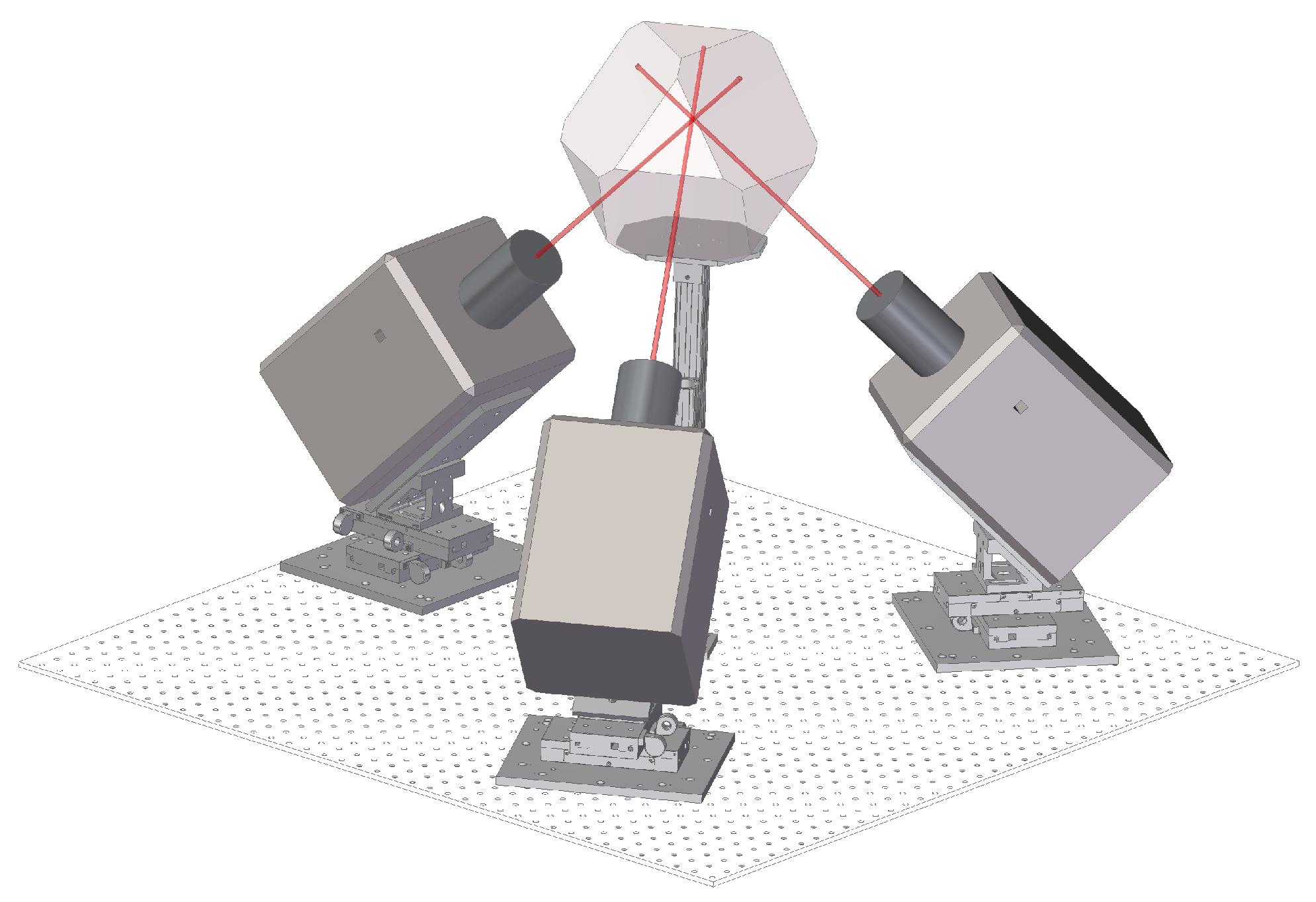
2.2. Experimental Setup
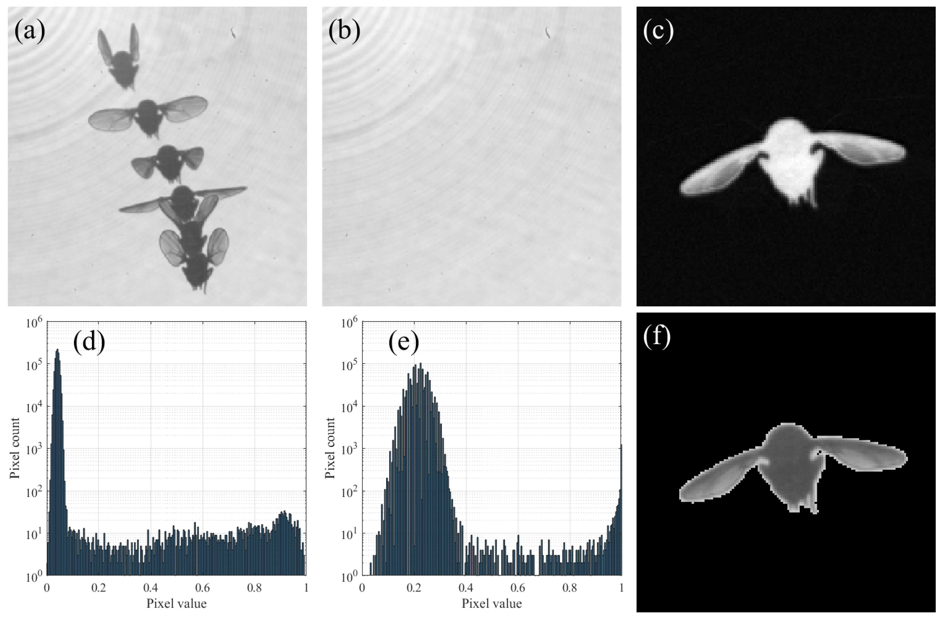
2.3. Background Subtraction
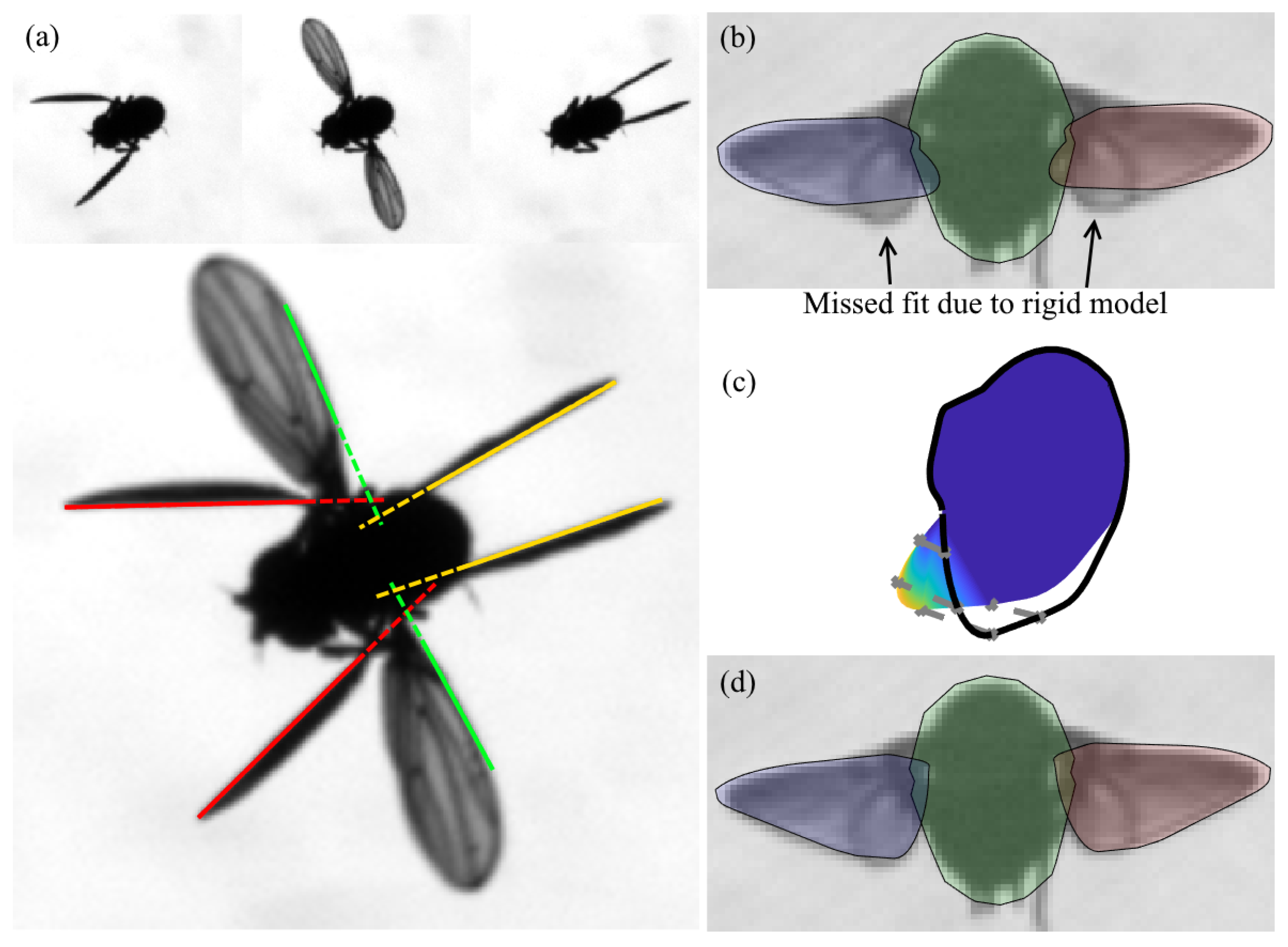
2.4. Generative Model
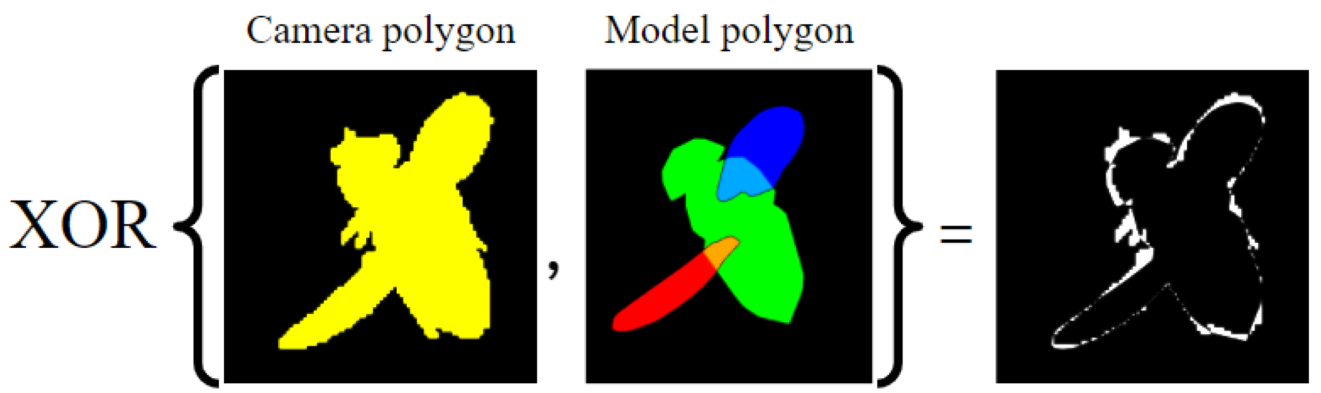
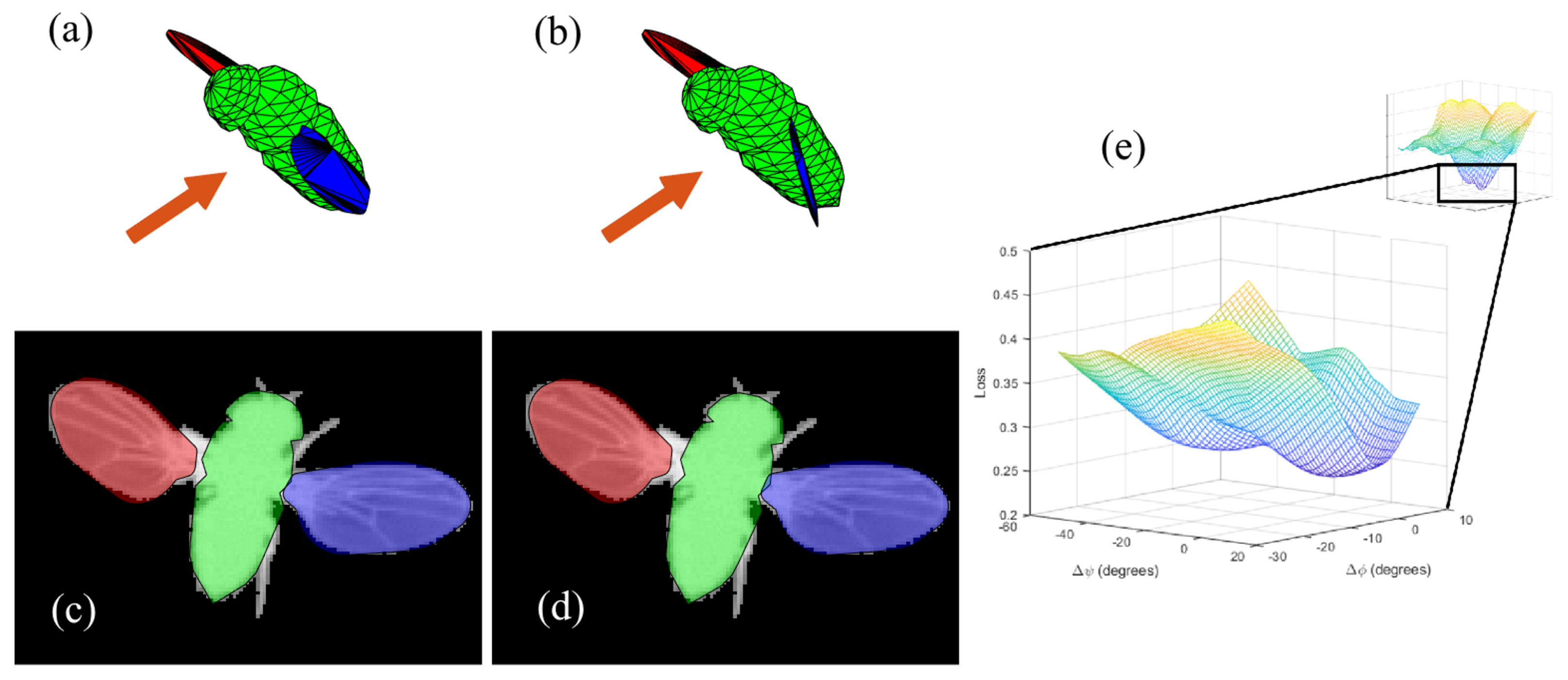
2.5. Loss Function Optimization
3. Results
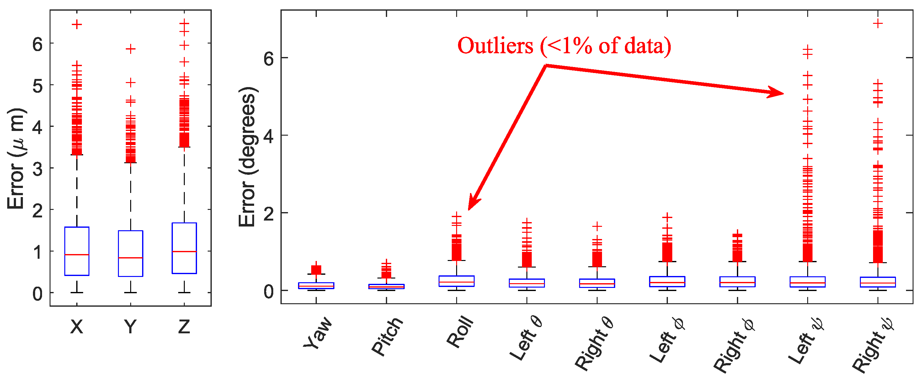
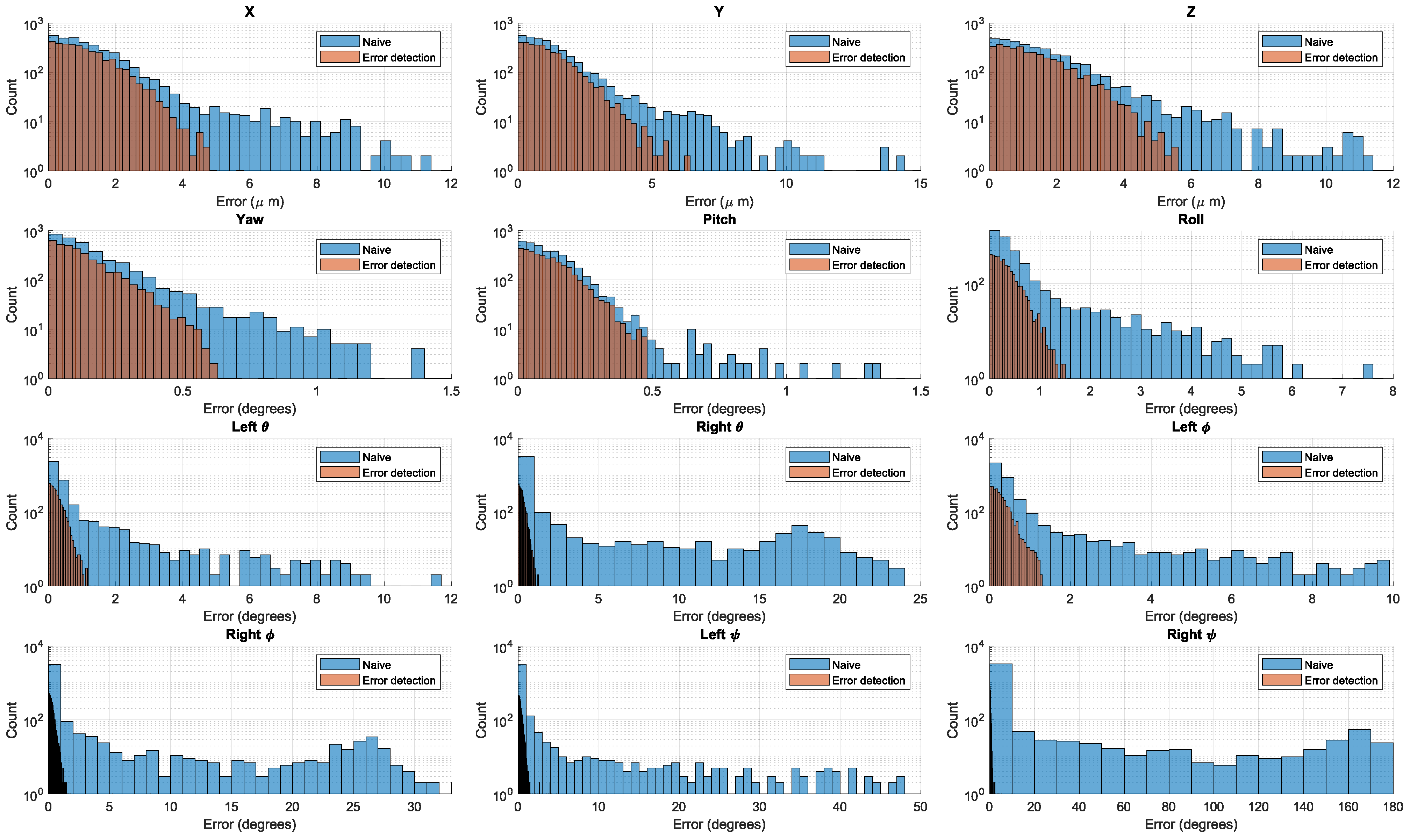
3.1. Validation
3.2. Non-Maneuvering Flight
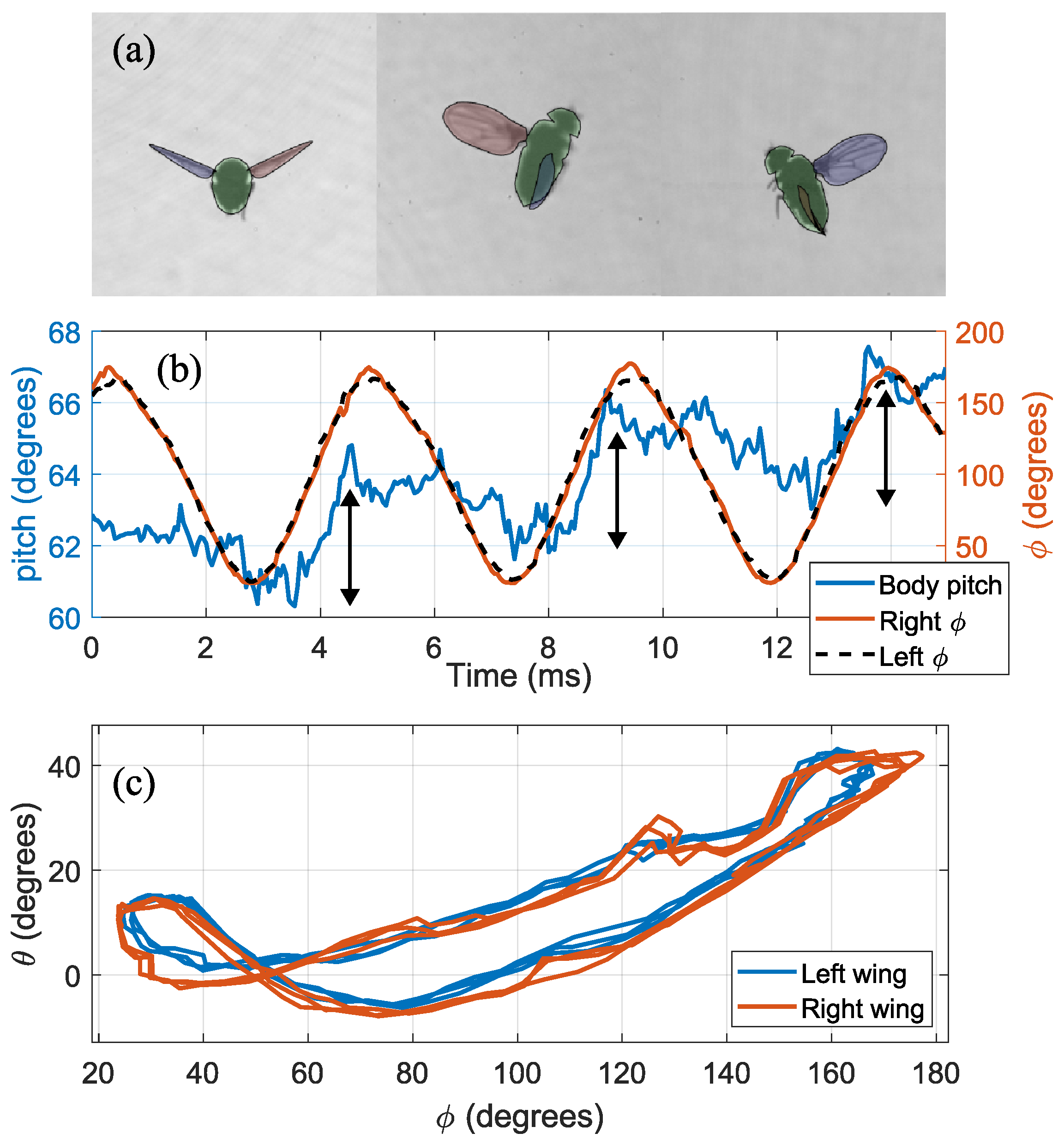
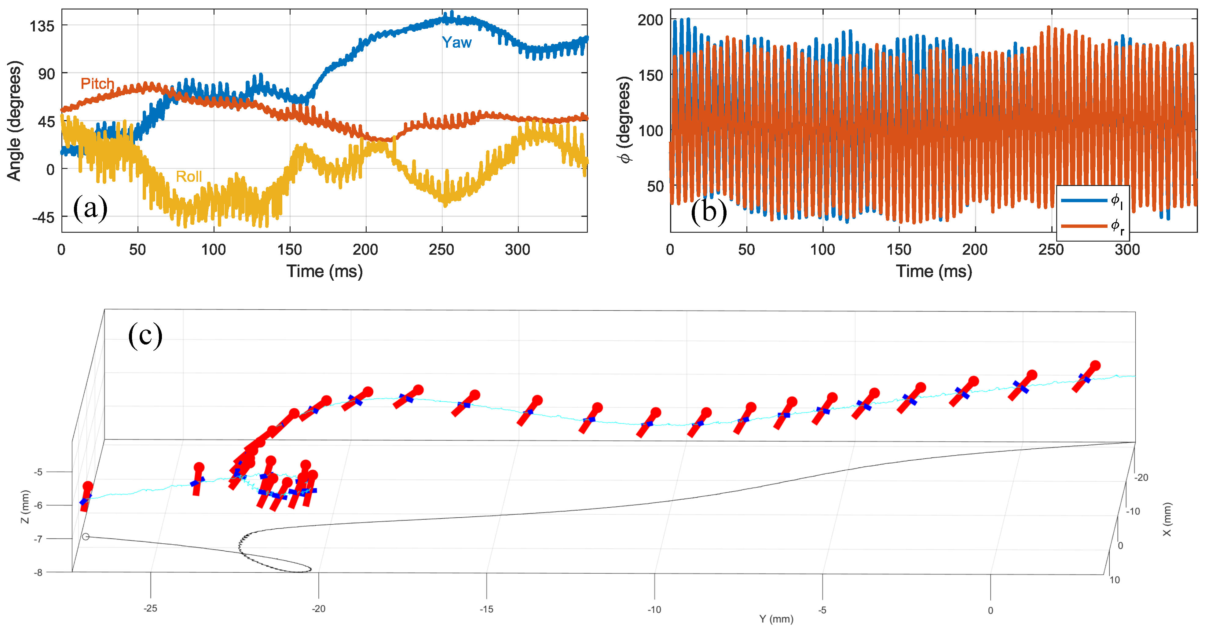
3.3. Free Flight Maneuver
3.4. Roll Correction Maneuver
4. Discussion and Conclusions
Supplementary Materials
Author Contributions
Funding
Data Availability Statement
Acknowledgments
Conflicts of Interest
Abbreviations
| DOF | degree of freedom |
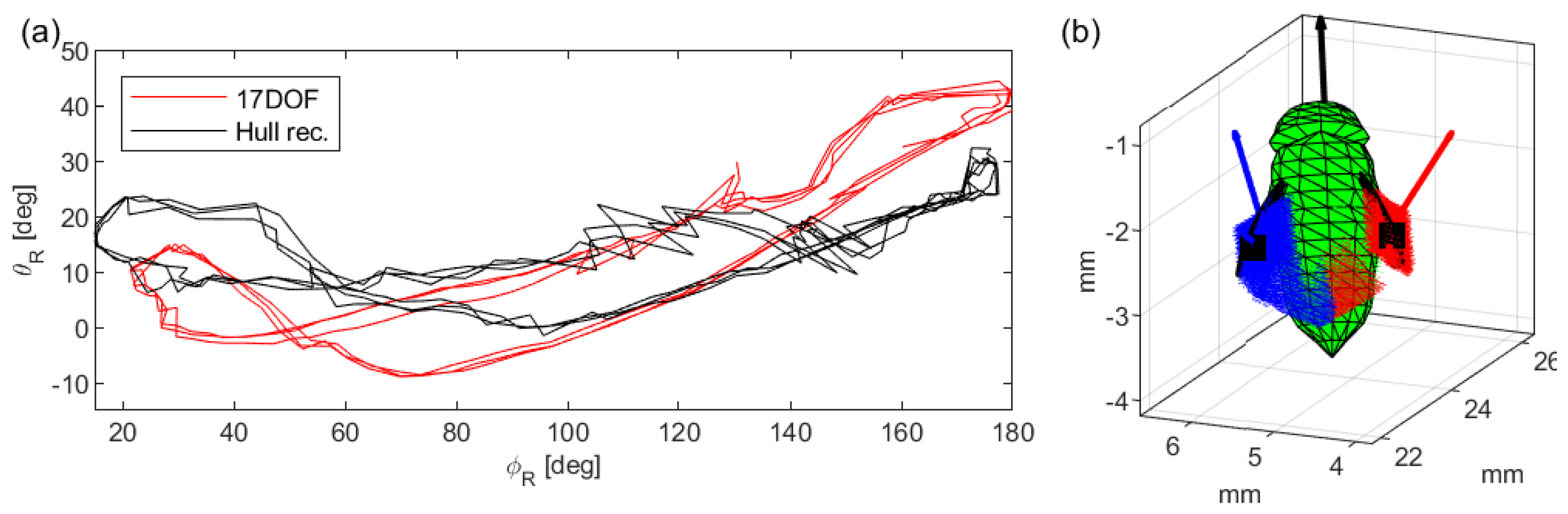
Appendix A. Comparison to 3-Camera Hull Reconstruction


References
- Dudley, R. The Biomechanics of Insect Flight: Form, Function, Evolution; Princeton University Press: Princeton, NJ, USA, 2002. [Google Scholar]
- Dickinson, M.H.; Muijres, F.T. The aerodynamics and control of free flight manoeuvres in Drosophila. Phil. Trans. R. Soc. B 2016, 371, 20150388. [Google Scholar] [CrossRef] [PubMed]
- Floreano, D.; Wood, R.J. Science, technology and the future of small autonomous drones. Nature 2015, 521, 460. [Google Scholar] [CrossRef] [PubMed]
- Fry, S.N.; Sayaman, R.; Dickinson, M.H. The aerodynamics of hovering flight in Drosophila. J. Exp. Biol. 2005, 208, 2303–2318. [Google Scholar] [CrossRef] [PubMed]
- Kassner, Z.; Dafni, E.; Ribak, G. Kinematic compensation for wing loss in flying damselflies. J. Insect Physiol. 2016, 85, 1–9. [Google Scholar] [CrossRef]
- Lyu, Y.Z.; Zhu, H.J.; Sun, M. Wing kinematic and aerodynamic compensations for unilateral wing damage in a small phorid fly. Phys. Rev. E 2020, 101, 012412. [Google Scholar] [CrossRef]
- Hedrick, T.L. Software techniques for two- and three-dimensional kinematic measurements of biological and biomimetic systems. Bioinspir. Biomim. 2008, 3, 034001. [Google Scholar] [CrossRef]
- Koehler, C.; Liang, Z.; Gaston, Z.; Wan, H.; Dong, H. 3D reconstruction and analysis of wing deformation in free-flying dragonflies. J. Exp. Biol. 2012, 215, 3018. [Google Scholar] [CrossRef]
- Nasir, N.; Mat, S. An automated visual tracking measurement for quantifying wing and body motion of free-flying houseflies. Measurement 2019, 143, 267–275. [Google Scholar] [CrossRef]
- Wang, H.; Zeng, L.; Yin, C. Measuring the body position, attitude and wing deformation of a free-flight dragonfly by combining a comb fringe pattern with sign points on the wing. Meas. Sci. Technol. 2002, 13, 903–908. [Google Scholar] [CrossRef]
- Ristroph, L.; Berman, G.J.; Bergou, A.J.; Wang, Z.J.; Cohen, I. Automated hull reconstruction motion tracking (HRMT) applied to sideways maneuvers of free-flying insects. J. Exp. Biol. 2009, 212, 1324–1335. [Google Scholar] [CrossRef]
- Walker, S.M.; Thomas, A.L.R.; Taylor, G.K. Operation of the alula as an indicator of gear change in hoverflies. J. R. Soc. Interface 2012, 9, 1194–1207. [Google Scholar] [CrossRef] [PubMed]
- Beatus, T.; Guckenheimer, J.; Cohen, I. Controlling roll perturbations in fruit flies. J. Roy. Soc. Interface 2015, 12, 20150075. [Google Scholar] [CrossRef] [PubMed]
- Whitehead, S.C.; Beatus, T.; Canale, L.; Cohen, I. Pitch perfect: How fruit flies control their body pitch angle. J. Exp. Biol. 2015, 218, 3508–3519. [Google Scholar] [CrossRef] [PubMed]
- Bomphrey, R.J.; Nakata, T.; Phillips, N.; Walker, S.M. Smart wing rotation and trailing-edge vortices enable high frequency mosquito flight. Nature 2017, 544, 92–95. [Google Scholar] [CrossRef]
- Fontaine, E.I.; Zabala, F.; Dickinson, M.H.; Burdick, J.W. Wing and body motion during flight initiation in Drosophila revealed by automated visual tracking. J. Exp. Biol. 2009, 212, 1307–1323. [Google Scholar] [CrossRef]
- Muijres, F.T.; Chang, S.W.; van Veen, W.G.; Spitzen, J.; Biemans, B.T.; Koehl, M.A.R.; Dudley, R. Escaping blood-fed malaria mosquitoes minimize tactile detection without compromising on take-off speed. J. Exp. Biol. 2017, 220, 3751–3762. [Google Scholar] [CrossRef]
- Kostreski, N.I. Automated Kinematic Extraction of Wing and Body Motions of Free Flying Diptera. Ph.D. Thesis, University of Maryland, College Park, MD, USA, 2012. [Google Scholar]
- Muijres, F.T.; Elzinga, M.J.; Melis, J.M.; Dickinson, M.H. Flies evade looming targets by executing rapid visually directed banked turns. Science 2014, 344, 172–177. [Google Scholar] [CrossRef]
- Wehmann, H.N.; Heepe, L.; Gorb, S.N.; Engels, T.; Lehmann, F.O. Local deformation and stiffness distribution in fly wings. Biol. Open 2019, 8, bio038299. [Google Scholar] [CrossRef]
- Theriault, D.H.; Fuller, N.W.; Jackson, B.E.; Bluhm, E.; Evangelista, D.; Wu, Z.; Betke, M.; Hedrick, T.L. A protocol and calibration method for accurate multi-camera field videography. J. Exp. Biol. 2014, 217, 1843–1848. [Google Scholar] [CrossRef]
- Ristroph, L.; Bergou, A.J.; Ristroph, G.; Coumes, K.; Berman, G.J.; Guckenheimer, J.; Wang, Z.J.; Cohen, I. Discovering the flight autostabilizer of fruit flies by inducing aerial stumbles. Proc. Natl. Acad. Sci. USA 2010, 107, 4820–4824. [Google Scholar] [CrossRef]
- Otsu, N. A Threshold Selection Method from Gray-Level Histograms. IEEE Trans. Syst. Man Cybern. 1979, 9, 62–66. [Google Scholar] [CrossRef]
- Beatus, T.; Cohen, I. Wing-pitch modulation in maneuvering fruit flies is explained by an interplay between aerodynamics and a torsional spring. Phys. Rev. E 2015, 92, 022712. [Google Scholar] [CrossRef] [PubMed]
- Nagesh, I.; Walker, S.M.; Taylor, G.K. Motor output and control input in flapping flight: A compact model of the deforming wing kinematics of manoeuvring hoverflies. J. R. Soc. Interface 2019, 16, 20190435. [Google Scholar] [CrossRef] [PubMed]
- Combes, S.; Daniel, T. Flexural stiffness in insect wings I. Scaling and the influence of wing venation. J. Exp. Biol. 2003, 206, 2979–2987. [Google Scholar] [CrossRef]
- Ma, Y.; Ma, T.; Ning, J.; Gorb, S. Structure and tensile properties of the forewing costal vein of the honeybee Apis mellifera. Soft Matter 2020, 16, 4057–4064. [Google Scholar] [CrossRef]
- Young, J.; Walker, S.M.; Bomphrey, R.J.; Taylor, G.K.; Thomas, A.L. Details of insect wing design and deformation enhance aerodynamic function and flight efficiency. Science 2009, 325, 1549–1552. [Google Scholar] [CrossRef]
- Arthur, D.; Vassilvitskii, S. k-means++: The advantages of careful seeding. In Proceedings of the Eighteenth Annual ACM-SIAM Symposium on Discrete Algorithms (SODA’07), New Orleans, LA, USA, 7–9 January 2007; Society for Industrial and Applied Mathematics: Philadelphia, PA, USA, 2007; pp. 1027–1035. [Google Scholar]
- Liu, S.; Li, T.; Chen, W.; Li, H. Soft rasterizer: A differentiable renderer for image-based 3d reasoning. In Proceedings of the IEEE/CVF International Conference on Computer Vision, Seoul, Korea, 27 October–2 November 2019; pp. 7708–7717. [Google Scholar]


| Name | Units | Description |
|---|---|---|
| mm | Center of mass position in the lab frame | |
| yaw | deg | Body azimuth angle (rotation around lab z) |
| pitch | deg | Body elevation angle |
| roll | deg | Body rotation around body x axis |
| deg | Wing stoke angles | |
| deg | Wing elevation angles | |
| deg | Wing pitch angles | |
| mm | Wing hinges translation in the body frame | |
| Wing twist per mm |
Publisher’s Note: MDPI stays neutral with regard to jurisdictional claims in published maps and institutional affiliations. |
© 2022 by the authors. Licensee MDPI, Basel, Switzerland. This article is an open access article distributed under the terms and conditions of the Creative Commons Attribution (CC BY) license (https://creativecommons.org/licenses/by/4.0/).
Share and Cite
Ben-Dov, O.; Beatus, T. Model-Based Tracking of Fruit Flies in Free Flight. Insects 2022, 13, 1018. https://doi.org/10.3390/insects13111018
Ben-Dov O, Beatus T. Model-Based Tracking of Fruit Flies in Free Flight. Insects. 2022; 13(11):1018. https://doi.org/10.3390/insects13111018
Chicago/Turabian StyleBen-Dov, Omri, and Tsevi Beatus. 2022. "Model-Based Tracking of Fruit Flies in Free Flight" Insects 13, no. 11: 1018. https://doi.org/10.3390/insects13111018
APA StyleBen-Dov, O., & Beatus, T. (2022). Model-Based Tracking of Fruit Flies in Free Flight. Insects, 13(11), 1018. https://doi.org/10.3390/insects13111018