


Response of Chironomids to Key Environmental Factors: Perspective for Biomonitoring


Abstract
Simple Summary
Abstract
1. Introduction
2. Materials and Methods
2.1. Chironomid Database
2.2. Data Analysis
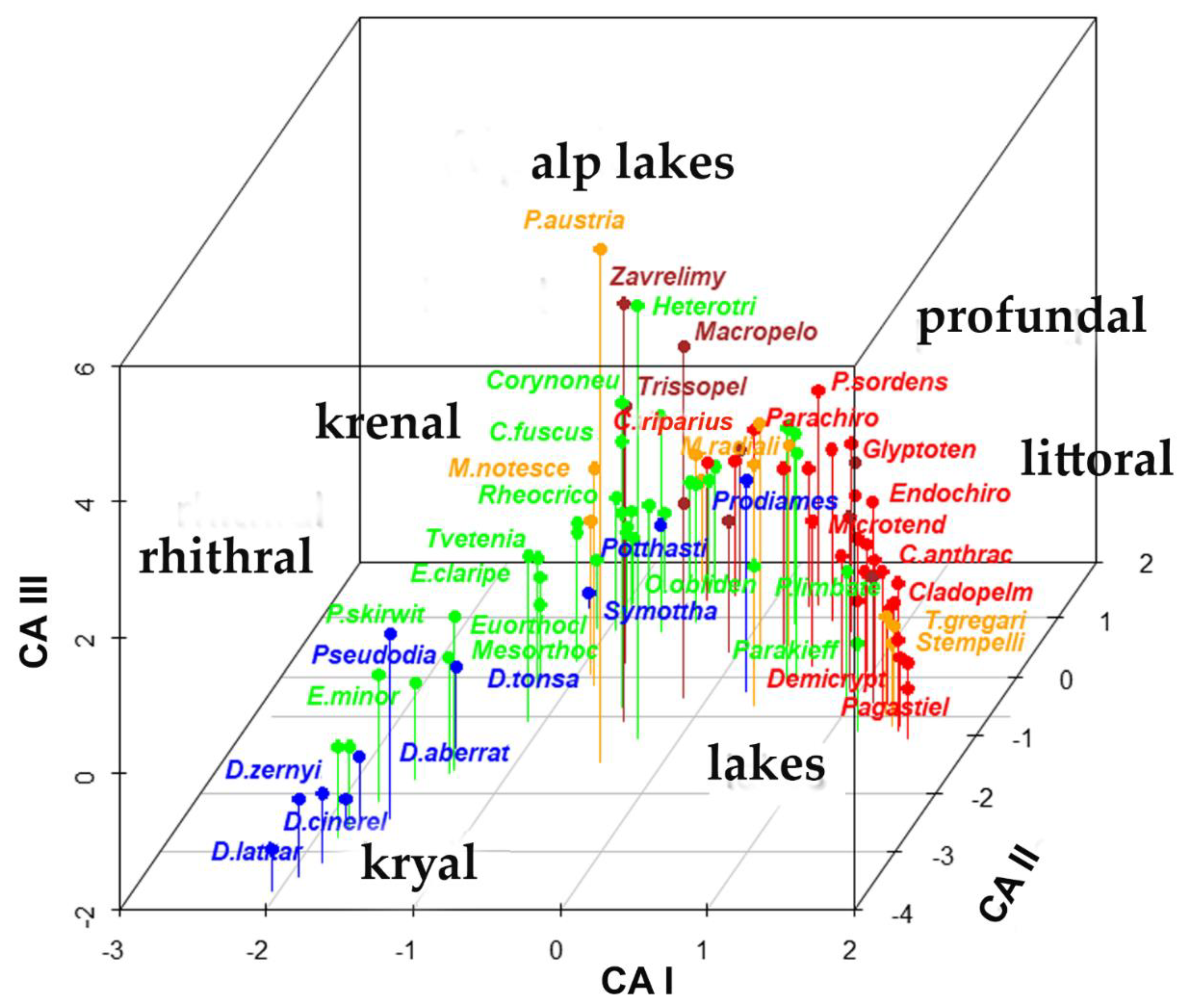
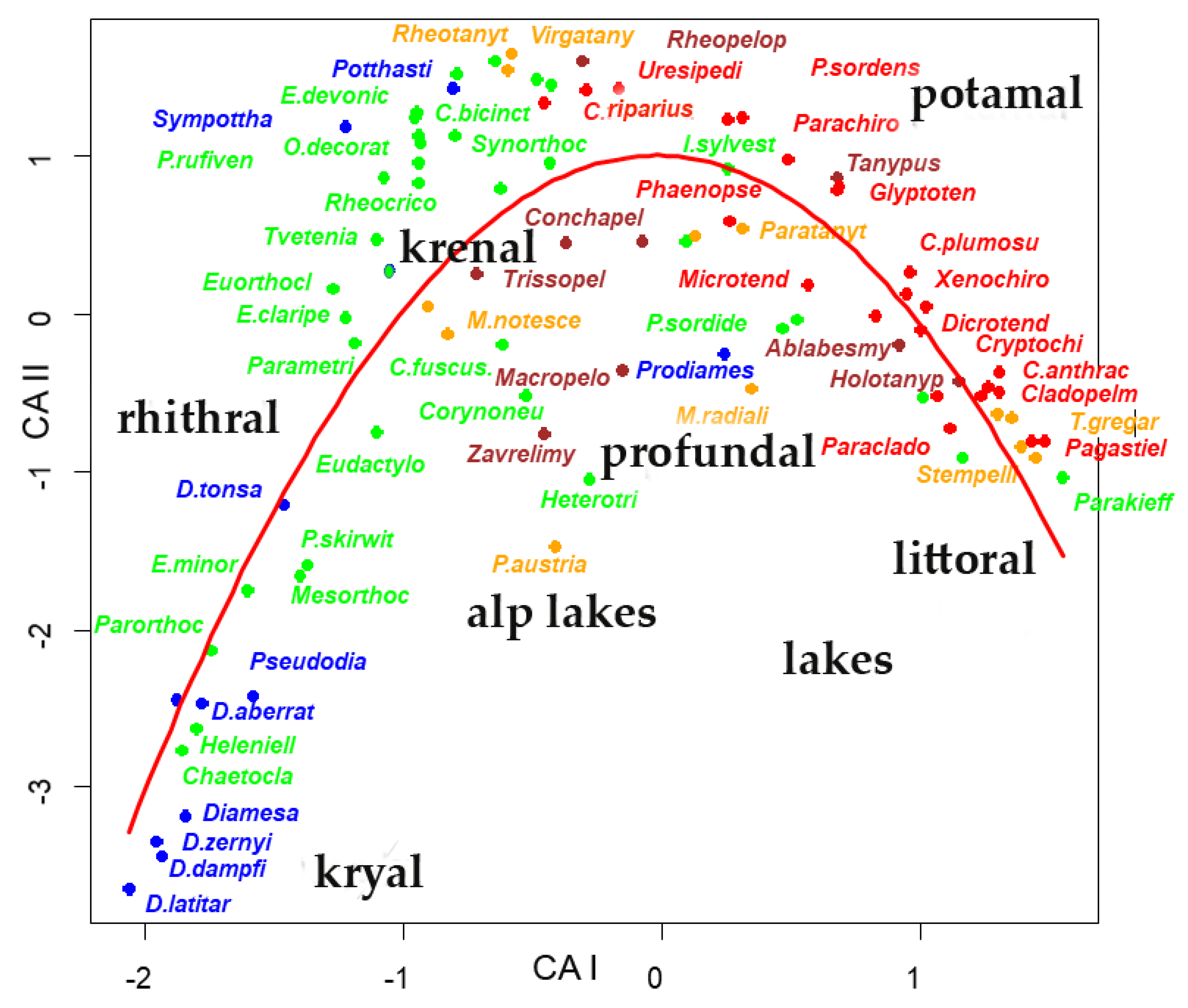
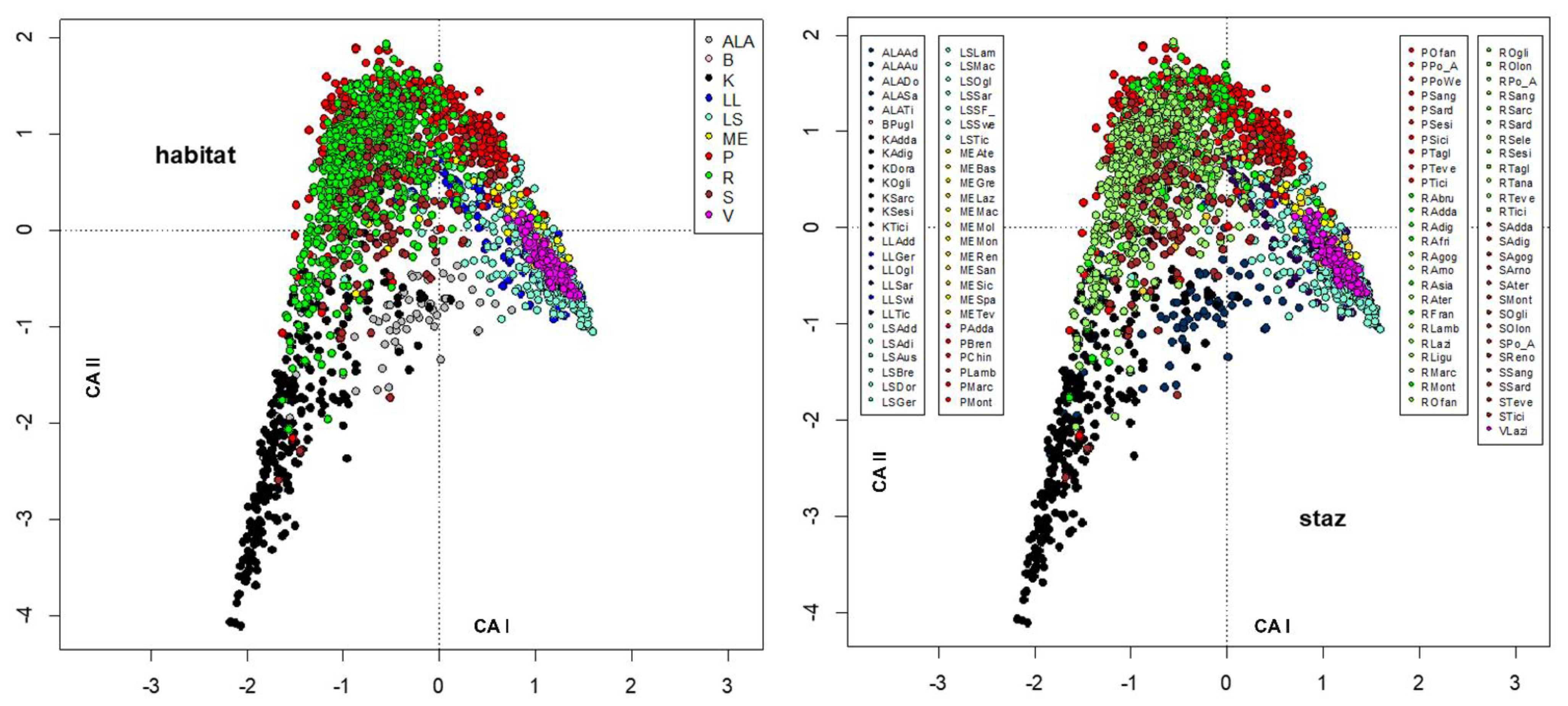
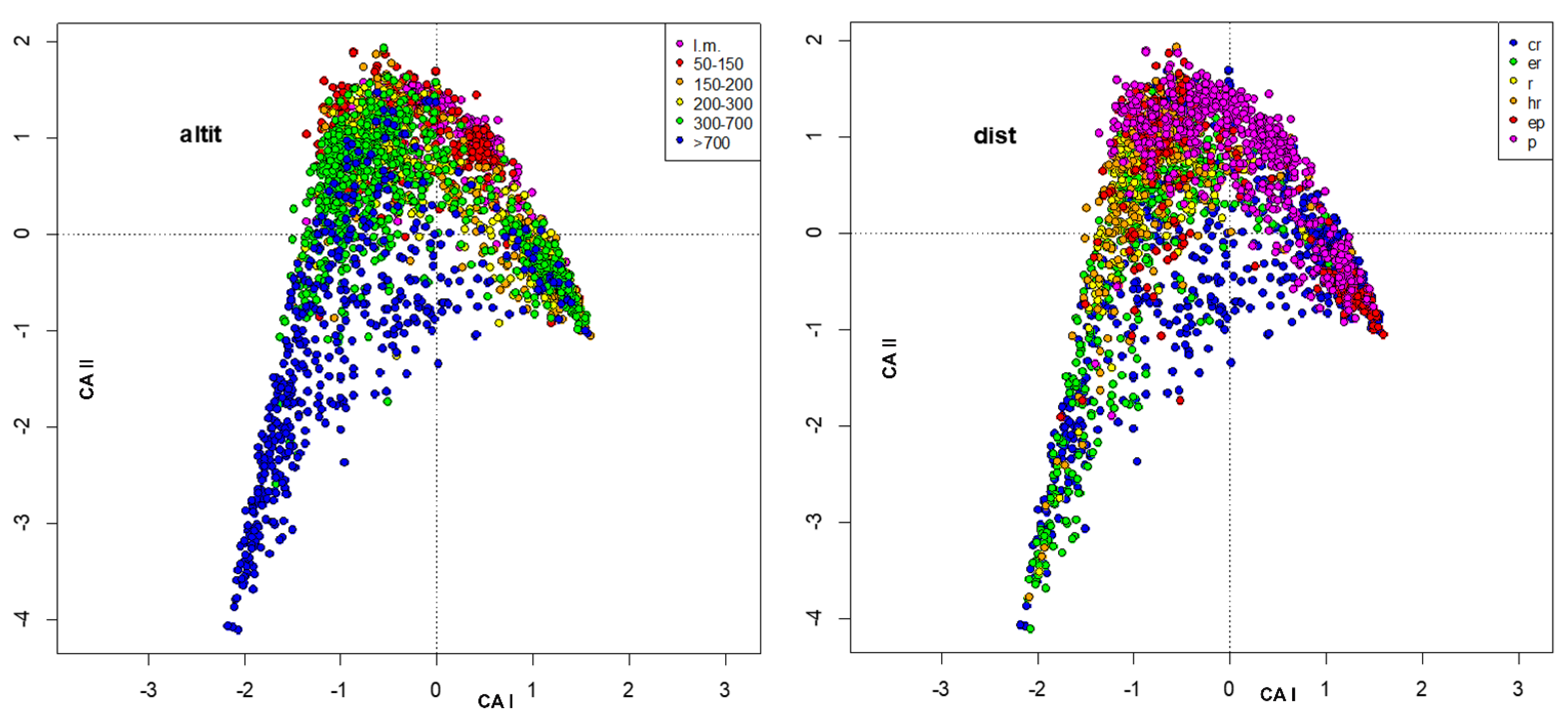
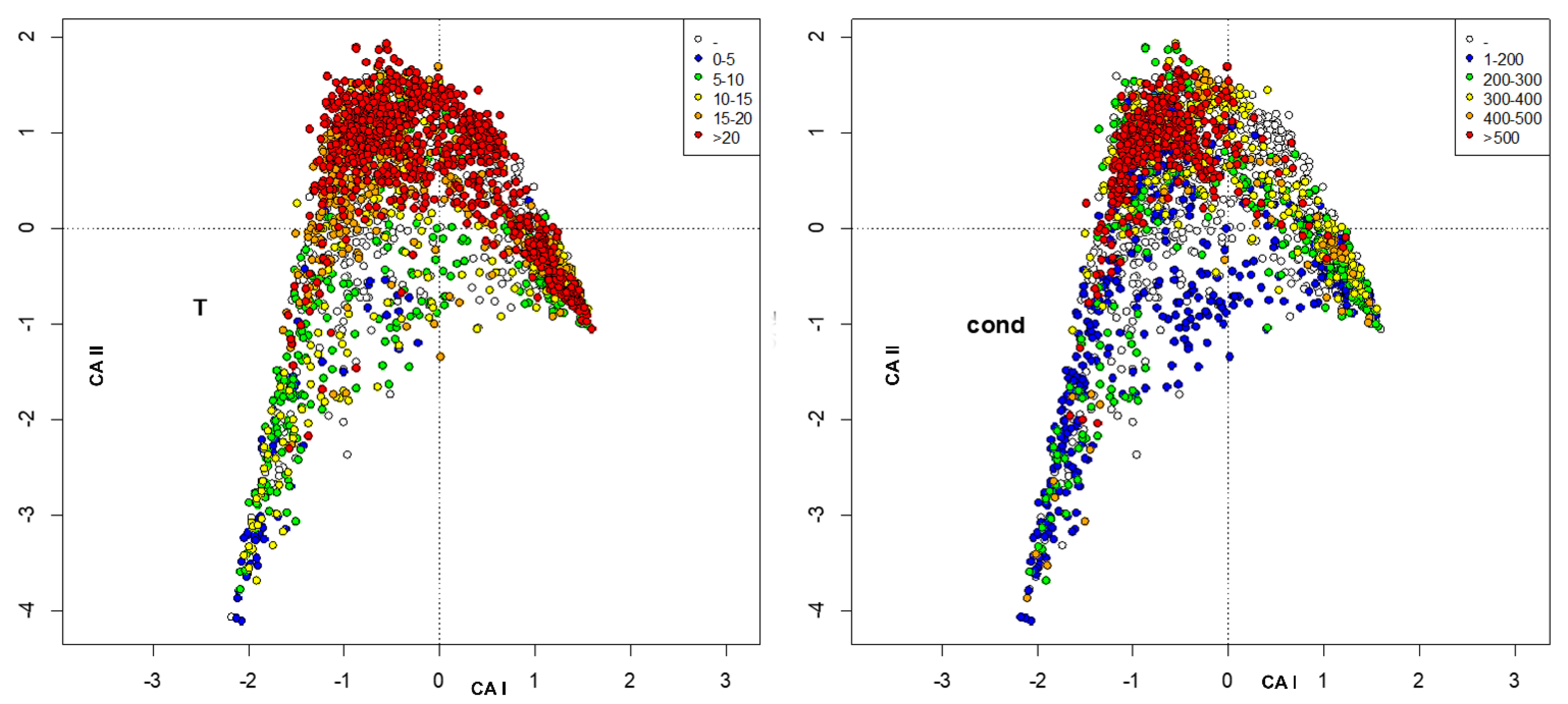
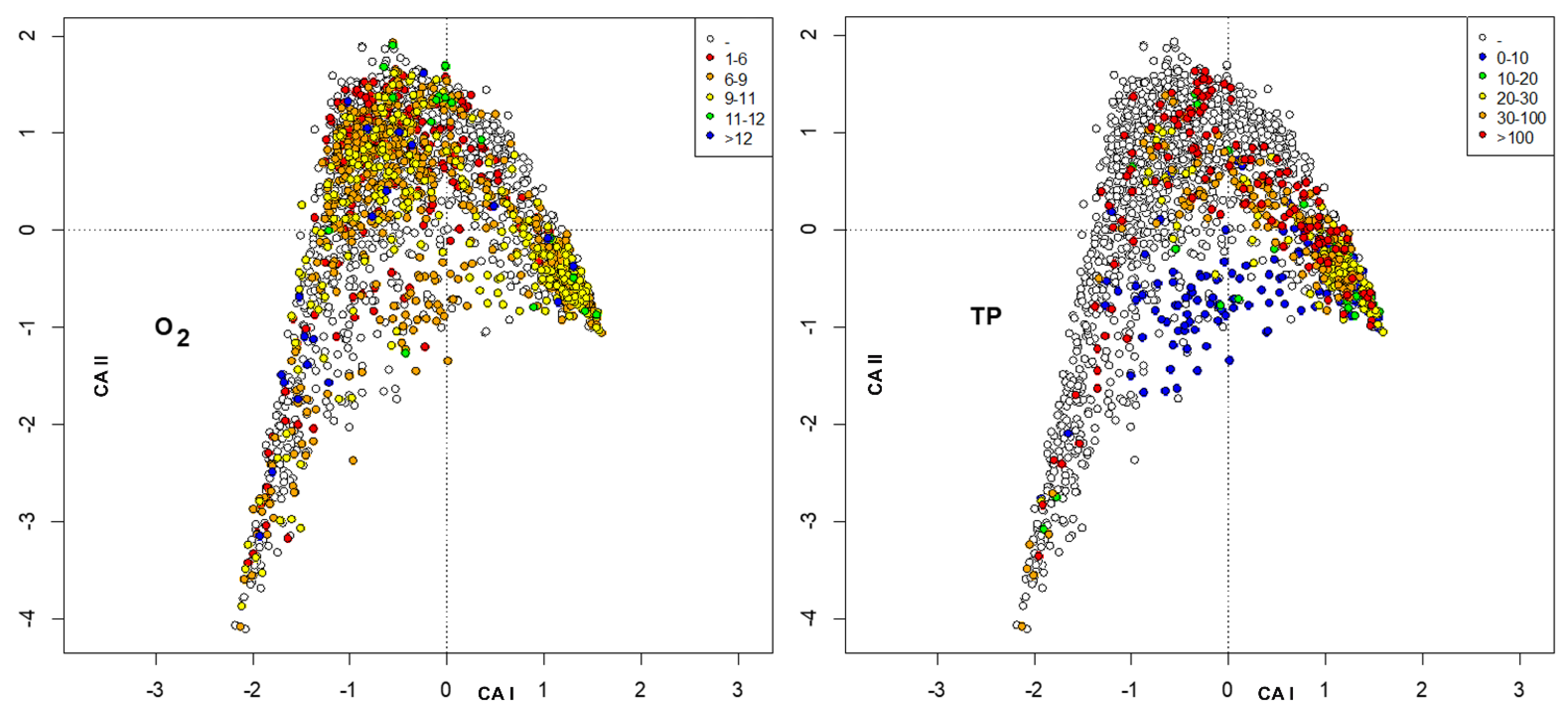
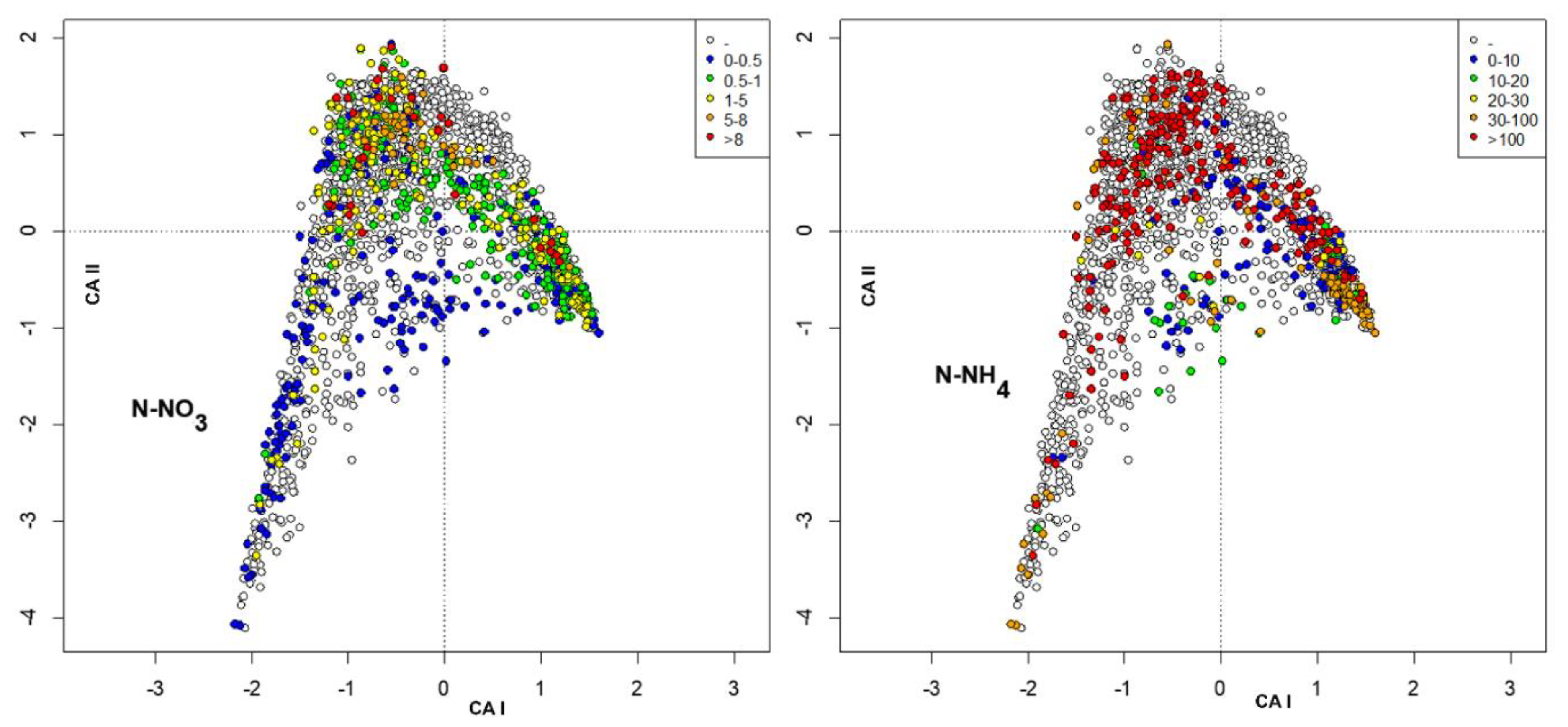
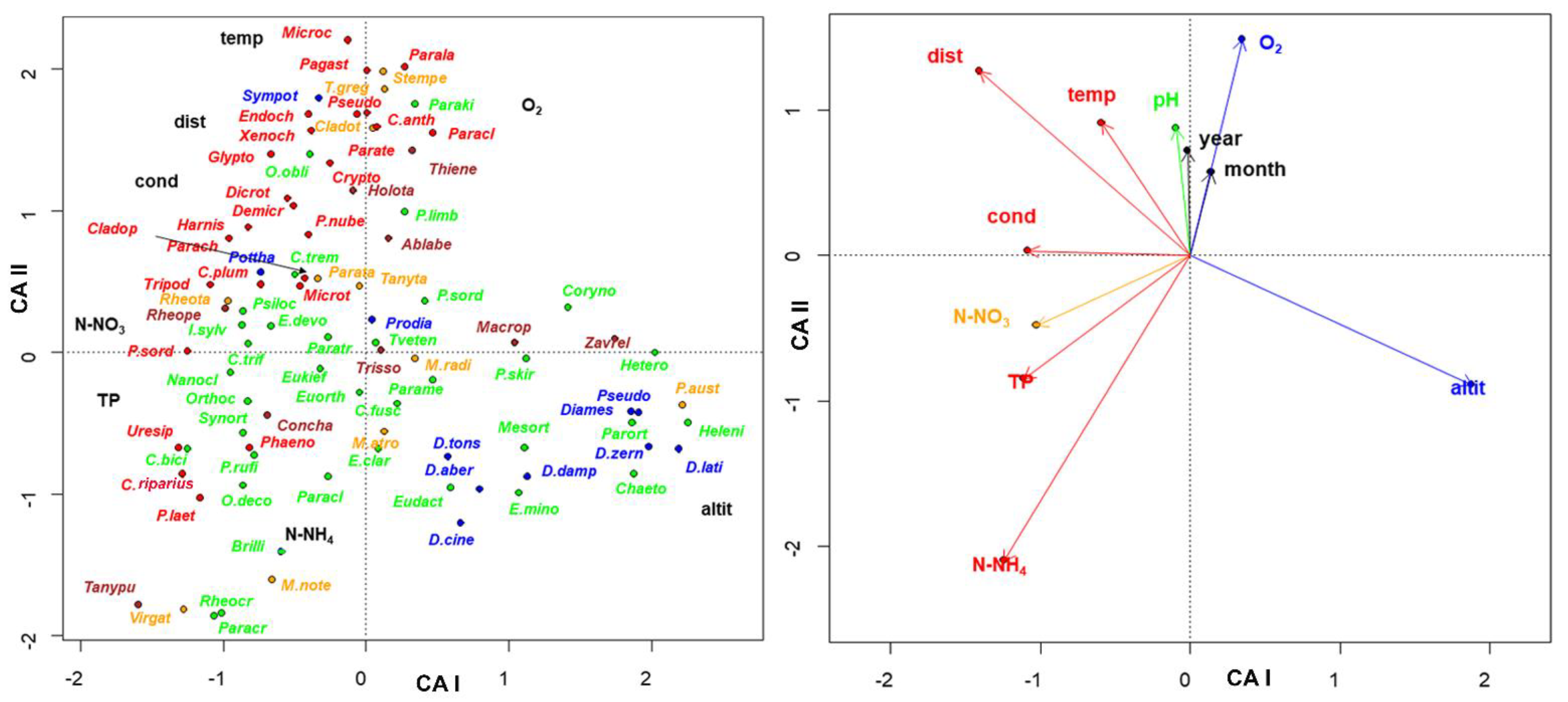
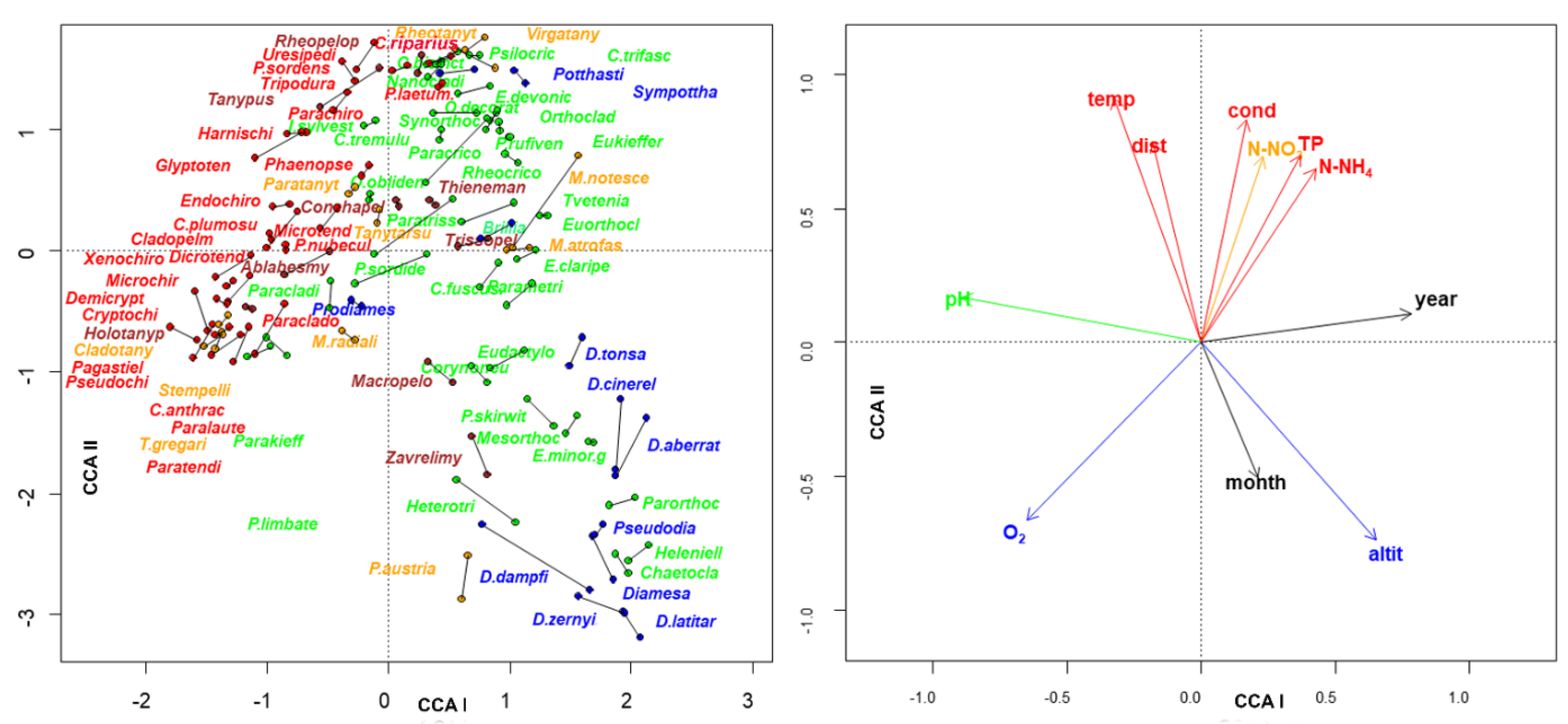
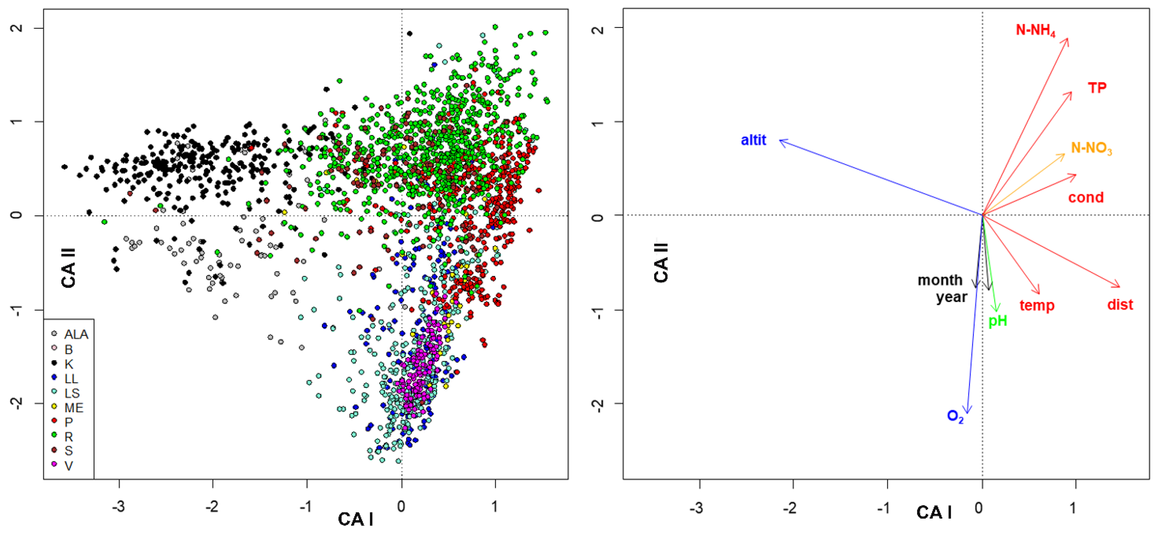
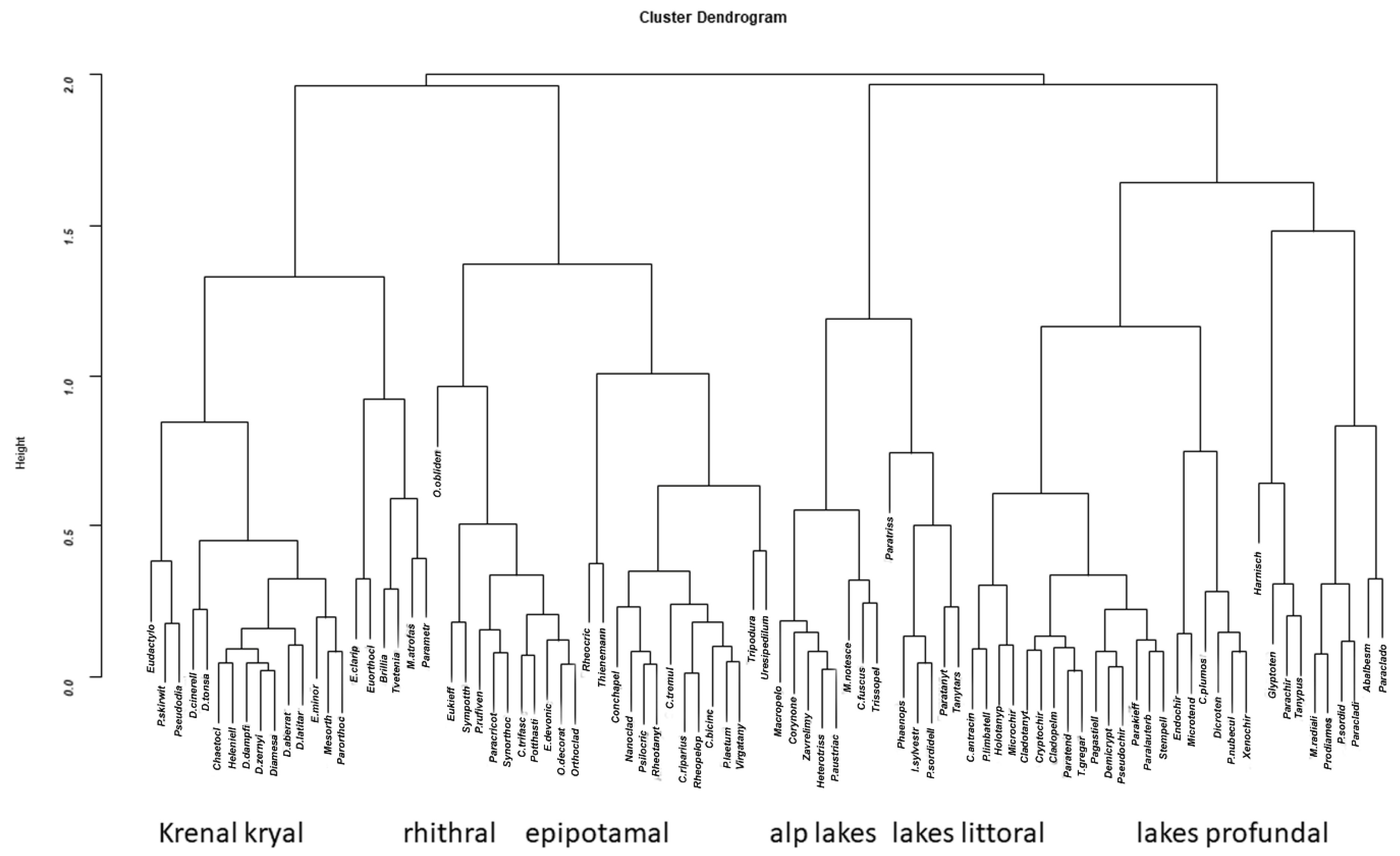
3. Results
4. Discussion
5. Conclusions
Supplementary Materials
Author Contributions
Funding
Institutional Review Board Statement
Data Availability Statement
Acknowledgments
Conflicts of Interest
References
- Li, L.; Zheng, B.; Liu, L. Biomonitoring and Bioindicators Used for River Ecosystems: Definitions, Approaches and Trends. Proc. Environ. Sci. 2010, 2, 1510–1524. [Google Scholar] [CrossRef]
- Armitage, P.D.; Cranston, P.S.; Pinder, L.C.V. Chironomidae: Biology and Ecology of Non-Biting Midges; Armitage, P.D., Cranston, P.S., Pinder, L.C.V., Eds.; Springer Science + Business Media, B.V.: Dordrecht, The Netherlands, 2012; ISBN 978-94-011-0715-0. [Google Scholar]
- Fornaroli, R.; Cabrini, R.; Zaupa, S.; Bettinetti, R.; Ciampittiello, M.; Boggero, A. Quantile Regression Analysis as a Predictive Tool for Lake Macroinvertebrate Biodiversity. Ecol. Indic. 2016, 61, 728–738. [Google Scholar] [CrossRef]
- Rossaro, B.; Marziali, L.; Montagna, M.; Magoga, G.; Zaupa, S.; Boggero, A. Factors Controlling Morphotaxa Distributions of Diptera Chironomidae in Freshwaters. Water 2022, 14, 1014. [Google Scholar] [CrossRef]
- Ni, Z.; Zhang, E.; Herzschuh, U.; Mischke, S.; Chang, J.; Sun, W.; Ning, D. Taxonomic and Functional Diversity Differentiation of Chironomid Communities in Northern Mongolian Plateau under Complex Environmental Impacts. Hydrobiologia 2020, 847, 2155–2167. [Google Scholar] [CrossRef]
- Sartori, L.; Canobbio, S.; Cabrini, R.; Fornaroli, R.; Mezzanotte, V. Macroinvertebrate Assemblages and Biodiversity Levels: Ecological Role of Constructed Wetlands and Artificial Ponds in a Natural Park. J. Limnol. 2015, 74, 335–345. [Google Scholar] [CrossRef]
- Free, G.; Solimini, A.; Rossaro, B.; Marziali, L.; Giacchini, R.; Paracchini, B.; Ghiani, M.; Vaccaro, S.; Gawlik, B.; Fresner, R.; et al. Modelling Lake Macroinvertebrate Species in the Shallow Sublittoral: Relative Roles of Habitat Lake Morphology Aquatic Chemistry and Sediment Composition. Hydrobiologia 2009, 633, 123–136. [Google Scholar] [CrossRef]
- Takamura, N.; Ito, T.; Ueno, R.; Ohtaka, A.; Wakana, I.; Nakagawa, M.; Ueno, Y.; Nakajima, H. Environmental Gradients Determining the Distribution of Benthic Macroinvertebrates in Lake Takkobu, Kushiro Wetland, Northern Japan. Ecol. Res. 2009, 24, 371–381. [Google Scholar] [CrossRef]
- Thienemann, A. Chironomus: Leben, Verbreitung und wirtschaftliche Bedeutung der Chironomiden; mit zahlr. Tabellen im Text. In Die Binnengewässer, 2nd ed.; Schweizerbart: Stuttgart, Germany, 1974; ISBN 978-3-510-40029-4. [Google Scholar]
- Tixier, G.; Wilson, K.P.; Williams, D.D. Exploration of the Influence of Global Warming on the Chironomid Community in a Manipulated Shallow Groundwater System. Hydrobiologia 2009, 624, 13–27. [Google Scholar] [CrossRef]
- Moore, J.W. Factors Influencing the Species Composition, Distribution and Abundance of Benthic Invertebrates in the Profundal Zone of a Eutrophic Northern Lake. Hydrobiologia 1981, 83, 505–510. [Google Scholar] [CrossRef]
- Verneaux, J.; Verneaux, V.; Guyard, A. Classification biologique des lacs jurassiens à l’aide d’une nouvelle méthode d’analyse des peuplements benthiques I. Variété et densité de la faune. Ann. Limnol. Int. J. Limnol. 1993, 29, 59–77. [Google Scholar] [CrossRef]
- Verneaux, V.; Verneaux, J.; Guyard, A. Classification biologique des lacs jurassiens à l’aide d’une nouvelle méthode d’analyse des peuplements benthiques II. Nature de la faune. Ann. Limnol. Int. J. Limnol. 1993, 29, 383–393. [Google Scholar] [CrossRef]
- Panis, L.I.; Goddeeris, B.; Verheyen, R. On the Relationship between Vertical Microdistribution and Adaptations to Oxygen Stress in Littoral Chironomidae (Diptera). Hydrobiologia 1996, 318, 61–67. [Google Scholar] [CrossRef]
- Boggero, A.; Zaupa, S.; Bettinetti, R.; Ciampittiello, M.; Fontaneto, D. The Benthic Quality Index to Assess Water Quality of Lakes May Be Affected by Confounding Environmental Features. Water 2020, 12, 2519. [Google Scholar] [CrossRef]
- Saether, O.A. Chironomid Communities as Water Quality Indicators. Ecography 1979, 2, 65–74. [Google Scholar] [CrossRef]
- Al-Shami, S.A.; Rawi, C.S.M.; HassanAhmad, A.; Nor, S.A.M. Distribution of Chironomidae (Insecta: Diptera) in Polluted Rivers of the Juru River Basin, Penang, Malaysia. J. Environ. Sci. 2010, 22, 1718–1727. [Google Scholar] [CrossRef]
- Resh, V.H.; Hildrew, A.G.; Statzner, B.; Townsend, C.R. Theoretical Habitat Templets, Species Traits, and Species Richness: A Synthesis of Long-Term Ecological Research on the Upper Rhone River in the Context of Concurrently Developed Ecological Theory. Freshw. Biol. 1994, 31, 539–554. [Google Scholar] [CrossRef]
- Doledec, S.; Statzner, B. Theoretical Habitat Templets, Species Traits, and Species Richness: 548 Plant and Animal Species in the Upper Rhone River and Its Floodplain. Freshw. Biol. 1994, 31, 523–538. [Google Scholar] [CrossRef]
- Statzner, B.; Hoppenhaus, K.; Arens, M.F.; Richoux, P. Reproductive Traits, Habitat Use and Templet Theory: A Synthesis of World-Wide Data on Aquatic Insects. Freshw. Biol. 1997, 38, 109–135. [Google Scholar] [CrossRef]
- Usseglio-Polatera, P.; Bournaud, M.; Richoux, P.; Tachet, H. Biological and Ecological Traits of Benthic Freshwater Macroinvertebrates: Relationships and Definition of Groups with Similar Traits. Freshw. Biol. 2000, 43, 175–205. [Google Scholar] [CrossRef]
- Serra, S.R.Q.; Cobo, F.; Graça, M.A.S.; Dolédec, S.; Feio, M.J. Synthesising the Trait Information of European Chironomidae (Insecta: Diptera): Towards a New Database. Ecol. Indic. 2016, 61, 282–292. [Google Scholar] [CrossRef]
- Jiang, X.; Pan, B.; Song, Z.; Xie, Z. Do Functional Traits of Chironomid Assemblages Respond More Readily to Eutrophication than Taxonomic Composition in Chinese Floodplain Lakes? Ecol. Indic. 2019, 103, 355–362. [Google Scholar] [CrossRef]
- Lemm, J.U.; Feld, C.K. Identification and Interaction of Multiple Stressors in Central European Lowland Rivers. Sci. Total Environ. 2017, 603–604, 148–154. [Google Scholar] [CrossRef] [PubMed]
- APAT & IRSA-CNR. Indice Biotico Esteso (I.B.E.). In Metodi Analitici per Le Acque. Indicatori Biologici; 3 sez. 9000; APAT & IRSA-CNR: Roma, Italy, 2003; pp. 1115–1136. [Google Scholar]
- Boggero, A.; Zaupa, S.; Cancellario, T.; Lencioni, V.; Marziali, L.; Rossaro, B. Italian Classification Method for Macroinvertebrates in Lakes Method Summary; CNR-Institute of Ecosystem: Verbania, Italy, 2017. [Google Scholar] [CrossRef]
- Rossaro, B.; Marziali, L.; Cardoso, A.C.; Solimini, A.; Free, G.; Giacchini, R. A Biotic Index Using Benthic Macroinvertebrates for Italian Lakes. Ecol. Indic. 2007, 7, 412–429. [Google Scholar] [CrossRef]
- Chaib, N.; Fouzari, A.; Bouhala, Z.; Samraoui, B.; Rossaro, B. Chironomid (Diptera, Chironomidae) Species Assemblages in Northeastern Algerian Hydrosystems. J. Entomol. Acarol. Res. 2013, 45, e2. [Google Scholar] [CrossRef]
- Buraschi, E.; Salerno, F.; Monguzzi, C.; Barbiero, G.; Tartari, G. Characterization of the Italian Lake-Types and Identification of Their Reference Sites Using Anthropogenic Pressure Factors. J. Limnol. 2005, 64, 75–84. [Google Scholar] [CrossRef]
- Tartari, G.; Buraschi, E.; Legnani, E.; Previtali, L.; Pagnotta, R.; Marchetto, A. Tipizzazione Dei Laghi Italiani Secondo Il Sistema B Della Direttiva 2000/60/CE. In Documento Presentato al Ministero dell’Ambiente e della Tutela del Territorio e del Mare; CNR-ISE: Roma, Italy, 2006; pp. 1–20. [Google Scholar]
- Braak, C.J.F.T.; Prentice, I.C. A Theory of Gradient Analysis. In Advances in Ecological Research; Elsevier: Amsterdam, The Netherlands, 1988; Volume 18, pp. 271–317. ISBN 978-0-12-013918-7. [Google Scholar]
- Legendre, P.; Legendre, L. Numerical Ecology Development in Environmental Modelling; Elsevier: Amsterdam, The Nethelands, 1998; Volume 20. [Google Scholar]
- R Core Team. R: A Language and Environment for Statistical Computing; The R Foundation: Vienna, Austria, 2018. [Google Scholar]
- Dixon, P. Vegan, a Package of R Functions for Community Ecology. J. Veg. Sci. 2003, 14, 927–930. [Google Scholar] [CrossRef]
- Van de Bund, W.; Solimini, A. Ecological Quality Ratios for Ecological Quality Assessment in Inland and Marine Waters; European Commission: Brussel, Belgium, 2007; pp. 1–24.
- Serra-Tosio, B. Ecologie et Biogéographie Des Diamesini d’Europe (Diptera, Chironomidae). Trav. Lab. Hydrobiol. Piscic. Univ. Grenoble. 1973, 63, 5–175. [Google Scholar]
- Larocque, I.; Hall, R.I.; Grahn, E. Chironomids as Indicators of Climate Change: A 100-lake Training Set from a Subarctic Region of Northern Sweden (Lapland). J. Paleolimnol. 2001, 26, 307–322. [Google Scholar] [CrossRef]
- Failla, A.J.; Vasquez, A.A.; Fujimoto, M.; Ram, J.L. The Ecological, Economic and Public Health Impacts of Nuisance Chironomids and Their Potential as Aquatic Invaders. Aqua. Invasions 2015, 9, 1–15. [Google Scholar] [CrossRef]
- Cranston, P.S.; Martin, J.; Spies, M. Cryptic Species in the Nuisance Midge Polypedilum Nubifer (Skuse) (Diptera: Chironomidae) and the Status of Tripedilum Kieffer. Zootaxa 2016, 4079, 429–447. [Google Scholar] [CrossRef]
- Rossaro, B. Chironomids and Water Temperature. Aqua. Insects 1991, 13, 87–98. [Google Scholar] [CrossRef]
- Marziali, L.; Rossaro, B. Response of Chironomid Species (Diptera, Chironomidae) to Water Temperature: Effects on Species Distribution in Specific Habitats. J. Entomol. Acarol. Res. 2013, 45, 14. [Google Scholar] [CrossRef]
- Brown, L.E.; Khamis, K.; Wilkes, M.; Blaen, P.; Brittain, J.E.; Carrivick, J.L.; Fell, S.; Friberg, N.; Füreder, L.; Gislason, G.M.; et al. Functional Diversity and Community Assembly of River Invertebrates Show Globally Consistent Responses to Decreasing Glacier Cover. Nat. Ecol. Evol. 2018, 2, 325–333. [Google Scholar] [CrossRef]
- Medeiros, A.S.; Milošević, Đ.; Francis, D.R.; Maddison, E.; Woodroffe, S.; Long, A.; Walker, I.R.; Hamerlík, L.; Quinlan, R.; Langdon, P.; et al. Arctic Chironomids of the Northwest North Atlantic Reflect Environmental and Biogeographic Gradients. J. Biogeogr. 2021, 48, 511–525. [Google Scholar] [CrossRef]
- Chevene, F.; Doleadec, S.; Chessel, D. A Fuzzy Coding Approach for the Analysis of Long-Term Ecological Data. Freshw. Biol. 1994, 31, 295–309. [Google Scholar] [CrossRef]
- Mabry, C.; Ackerly, D.; Gerhardt, F. Landscape and Species-Level Distribution of Morphological and Life History Traits in a Temperate Woodland Flora. J. Veg. Sci. 2000, 11, 213–224. [Google Scholar] [CrossRef]
- Gayraud, S.; Statzner, B.; Bady, P.; Haybachp, A.; Schöll, F.; Usseglio-Polatera, P.; Bacchi, M. Invertebrate Traits for the Biomonitoring of Large European Rivers: An Initial Assessment of Alternative Metrics: Invertebrate Traits and Human Impacts. Freshw. Biol. 2003, 48, 2045–2064. [Google Scholar] [CrossRef]
- Serra, S.R.Q.; Graça, M.A.S.; Dolédec, S.; Feio, M.J. Chironomidae Traits and Life History Strategies as Indicators of Anthropogenic Disturbance. Environ. Monit. Assess. 2017, 189, 326. [Google Scholar] [CrossRef] [PubMed]
- Rossaro, B. Factors That Determine Chironomid Species Distribution in Fresh Waters. Boll. Zool. 1991, 58, 281–286. [Google Scholar] [CrossRef]
- Rossaro, B.; Boggero, A.; Crozet, B.L.; Free, G.; Lencioni, V.; Marziali, L. A Comparison of Different Biotic Indices Based on Benthic Macro-Invertebrates in Italian Lakes. J. Limnol. 2011, 70, 109–122. [Google Scholar] [CrossRef]
- Serra, S.R.Q.; Graça, M.A.S.; Dolédec, S.; Feio, M.J. Discriminating Permanent from Temporary Rivers with Traits of Chironomid Genera. Ann. Limnol. Int. J. Limnol. 2017, 53, 161–174. [Google Scholar] [CrossRef]
- van Kleef, H.; Verberk, W.C.E.P.; Kimenai, F.F.P.; van der Velde, G.; Leuven, R.S.E.W. Natural Recovery and Restoration of Acidified Shallow Soft-Water Lakes: Successes and Bottlenecks Revealed by Assessing Life-History Strategies of Chironomid Larvae. Basic Appl. Ecol. 2015, 16, 325–334. [Google Scholar] [CrossRef]
- Serra, S.R.Q.; Graça, M.A.S.; Dolédec, S.; Feio, M.J. Chironomidae of the Holarctic Region: A Comparison of Ecological and Functional Traits between North America and Europe. Hydrobiologia 2017, 794, 273–285. [Google Scholar] [CrossRef]
- Bonada, N.; Dolédec, S. Does the Tachet Trait Database Report Voltinism Variability of Aquatic Insects between Mediterranean and Scandinavian Regions? Aqua. Sci. 2017, 80, 7. [Google Scholar] [CrossRef]
- Feio, M.J.; Dolédec, S. Integration of Invertebrate Traits into Predictive Models for Indirect Assessment of Stream Functional Integrity: A Case Study in Portugal. Ecol. Indic. 2012, 15, 236–247. [Google Scholar] [CrossRef]
- Legendre, P.; Galzin, R.; Harmelin-Vivien, M.L. Relating Behavior to Habitat: Solutions to The fourth-Corner Problem. Ecology 1997, 78, 547–562. [Google Scholar] [CrossRef]
- Dray, S.; Legendre, P. Testing the Species Traits–Environment Relationships: The Fourth-Corner Problem Revisited. Ecology 2008, 89, 3400–3412. [Google Scholar] [CrossRef] [PubMed]
- Reiss, F. Ökologische Und Systematische Untersuchungen an Chironomiden (Diptera) Des Bodensees. Ein Beitrag Zur Lakustrischen Chironomidenfauna des Nördlichen Alpenvorlandes. Arch. Hydrobiol. 1968, 64, 176–323. [Google Scholar]
- Brown, A.M.; Warton, D.I.; Andrew, N.R.; Binns, M.; Cassis, G.; Gibb, H. The Fourth-Corner Solution—Using Predictive Models to Understand How Species Traits Interact with the Environment. Methods Ecol. Evol. 2014, 5, 344–352. [Google Scholar] [CrossRef]


| Alt | Dist | Year | Month | Temp | pH | Cond | O2 | N-NO3 | TP | N-NH4 |
|---|---|---|---|---|---|---|---|---|---|---|
| 9127 | 7546 | 9127 | 9045 | 5951 | 4797 | 4823 | 5335 | 3530 | 2854 | 2045 |
| Species\Environmental Variables | Alt | Dist | Year | Month | Temp | pH | Cond | O2 | N-NO3 | TP | N-NH4 | |||||||||||
|---|---|---|---|---|---|---|---|---|---|---|---|---|---|---|---|---|---|---|---|---|---|---|
| Ablabesmyia spp. | + | * | − | * | + | * | + | − | * | + | * | − | * | + | * | − | − | * | − | |||
| Brillia spp. | − | − | − | + | − | − | * | − | * | − | + | − | − | |||||||||
| Chaetocladius spp. | + | * | − | * | + | * | + | − | − | * | − | + | − | + | − | |||||||
| Chironomus (Chironomus) anthracinus | + | * | − | + | + | − | + | * | − | + | − | − | − | |||||||||
| Chironomus (Chironomus) plumosus | + | * | − | * | − | * | − | * | − | * | + | * | − | + | * | + | − | * | − | |||
| Chironomus (Chironomus) riparius | + | − | + | + | − | + | * | − | − | + | + | − | ||||||||||
| Cladopelma spp. | + | − | * | + | + | * | + | + | − | + | − | − | − | |||||||||
| Cladotanytarsus spp. | + | * | − | * | − | − | − | * | + | * | − | + | * | + | − | − | * | |||||
| Conchapelopia spp. | + | − | − | * | + | − | * | + | * | + | + | * | − | − | * | − | * | |||||
| Corynoneura spp. | + | * | − | + | * | + | * | − | * | − | − | * | + | − | * | − | * | − | * | |||
| Cricotopus (Cricotopus) bicinctus | − | − | + | − | − | * | + | + | + | * | + | − | − | |||||||||
| Cricotopus (Cricotopus) fuscus | + | * | − | + | − | − | * | + | − | + | − | − | − | * | ||||||||
| Cricotopus (Cricotopus) tremulus | − | − | − | − | − | − | + | + | − | − | − | |||||||||||
| Cricotopus (Cricotopus) trifascia | − | + | − | − | − | + | + | + | + | − | − | |||||||||||
| Cricotopus (Isocladius) sylvestris | − | − | − | * | − | − | + | − | + | − | − | − | ||||||||||
| Cricotopus (Paratrichocladius) rufiventris | − | − | + | * | − | + | + | − | − | + | + | + | ||||||||||
| Cricotopus (Paratrichocladius) skirwithensis | − | + | + | − | − | + | − | − | − | − | − | |||||||||||
| Cryptochironomus spp. | + | * | − | * | − | * | − | − | * | + | * | − | * | + | * | − | − | * | − | * | ||
| Demicryptochironomus spp. | − | − | − | * | + | − | − | − | + | − | + | + | ||||||||||
| Diamesa aberrata | + | + | + | + | − | − | + | + | + | − | − | |||||||||||
| Diamesa cinerella | − | + | + | − | + | + | − | − | − | − | − | |||||||||||
| Diamesa dampfi | + | − | + | + | − | + | − | + | − | − | − | |||||||||||
| Diamesa latitarsis | + | * | − | * | + | * | + | − | * | − | * | − | * | + | − | − | − | |||||
| Diamesa spp. | + | * | − | + | * | + | − | * | − | − | * | + | − | − | − | |||||||
| Diamesa tonsa | + | * | − | + | + | − | * | − | * | − | * | + | − | − | − | * | ||||||
| Diamesa zernyi | + | * | − | + | * | + | − | * | − | * | − | * | + | − | * | − | − | |||||
| Dicrotendipes spp. | + | * | − | * | + | − | − | * | − | − | + | * | − | * | − | * | − | * | ||||
| Endochironomus spp. | + | * | − | * | − | + | − | + | − | + | − | − | * | − | ||||||||
| Eukiefferiella claripennis | + | * | − | * | + | − | − | − | * | − | − | − | − | − | ||||||||
| Eukiefferiella devonica | − | + | + | * | + | + | + | − | + | − | + | − | ||||||||||
| Eukiefferiella minor | + | * | − | + | * | + | − | * | − | * | − | * | − | − | * | − | − | |||||
| Eukiefferiella spp. | + | + | + | − | + | + | − | − | + | − | − | |||||||||||
| Glyptotendipes spp. | + | − | + | + | − | + | * | − | * | − | − | − | − | |||||||||
| Harnischia spp. | + | * | − | * | + | * | − | − | * | + | * | − | + | * | − | − | * | − | ||||
| Heleniella spp. | + | * | − | + | * | + | − | − | − | * | + | − | − | − | ||||||||
| Heterotrissocladius marcidus | + | * | − | + | * | + | * | − | * | − | − | * | + | * | − | * | − | − | * | |||
| Macropelopia spp. | + | * | + | + | * | + | − | * | − | − | * | + | − | − | − | |||||||
| Microchironomus spp. | − | + | − | − | − | + | − | + | * | − | − | − | * | |||||||||
| Micropsectra atrofasciata | + | * | − | * | + | * | − | − | * | − | * | − | * | − | − | * | − | * | − | |||
| Micropsectra notescens | + | + | + | − | + | + | + | − | + | + | + | |||||||||||
| Micropsectra radialis | + | + | − | − | − | + | − | * | + | * | − | − | − | |||||||||
| Microtendipes spp. | + | − | − | * | − | − | + | * | − | + | * | − | − | − | ||||||||
| Nanocladius spp. | − | − | + | + | + | − | * | + | − | − | − | − | ||||||||||
| Orthocladius (Eudactylocladius) spp. | + | + | * | + | * | − | − | − | − | + | − | − | − | |||||||||
| Orthocladius (Euorthocladius) spp. | + | * | − | * | + | * | − | − | − | * | + | − | − | − | * | − | * | |||||
| Orthocladius (Mesorthocladius) spp. | + | * | − | + | * | + | − | * | − | − | * | − | − | − | − | |||||||
| Orthocladius (Orthocladius) decoratus | + | − | * | + | * | − | − | − | + | + | + | − | − | |||||||||
| Orthocladius (Orthocladius) oblidens | + | − | − | * | − | − | * | − | − | + | − | − | * | − | ||||||||
| Orthocladius (Orthocladius) spp. | − | − | + | * | − | * | + | + | + | − | − | − | − | |||||||||
| Pagastiella orophila | + | − | * | + | − | − | + | + | * | + | − | − | − | |||||||||
| Parachironomus spp. | − | − | − | * | − | − | + | + | + | + | − | − | ||||||||||
| Paracladius spp. | + | − | + | + | − | + | − | + | − | − | + | |||||||||||
| Paracladopelma spp. | + | * | − | * | + | * | − | * | − | + | − | + | + | * | + | − | ||||||
| Paracricotopus niger | − | − | + | − | + | − | + | − | − | + | + | |||||||||||
| Parakiefferiella spp. | − | + | + | − | + | + | − | + | * | + | − | − | ||||||||||
| Paralauterborniella nigrohalteralis | + | * | − | * | + | * | − | − | * | + | * | + | + | + | − | − | ||||||
| Parametriocnemus spp. | + | * | − | + | * | + | − | * | − | * | − | + | − | − | − | |||||||
| Paratanytarsus austriacus | + | − | + | + | − | + | − | + | − | − | + | |||||||||||
| Paratanytarsus spp. | + | * | − | * | − | − | − | + | − | + | * | − | − | − | ||||||||
| Paratendipes spp. | − | * | − | * | − | * | − | * | − | + | * | − | + | * | − | − | * | − | ||||
| Paratrissocladius excerptus | + | + | + | − | + | − | + | − | + | − | − | |||||||||||
| Parorthocladius nudipennis | + | * | − | + | * | + | − | * | − | − | * | + | − | − | − | |||||||
| Phaenopsectra flavipes | + | * | − | + | − | − | + | − | + | * | − | − | * | − | ||||||||
| Polypedilum (Pentapedilum) sordens | − | + | − | − | − | + | + | − | − | − | + | |||||||||||
| Polypedilum (Polypedilum) laetum | + | − | + | + | − | + | + | + | + | − | − | |||||||||||
| Polypedilum (Polypedilum) nubeculosum | + | − | * | − | * | − | − | + | * | − | * | + | * | − | − | − | * | |||||
| Polypedilum (Tripodura) spp. | + | * | − | * | + | * | + | − | + | + | + | − | − | − | ||||||||
| Polypedilum (Uresipedilum) spp. | + | − | − | − | − | + | + | + | − | − | − | |||||||||||
| Potthastia spp. | − | − | + | * | − | + | + | − | − | − | − | − | ||||||||||
| Procladius (Holotanypus) choreus | + | − | * | − | − | − | * | + | * | − | * | + | * | − | − | * | − | * | ||||
| Prodiamesa spp. | + | + | * | + | + | − | * | + | * | − | * | + | − | − | − | |||||||
| Psectrocladius (Psectrocladius) limbatellus | + | − | * | − | * | − | − | * | + | − | * | + | * | − | − | − | ||||||
| Psectrocladius (Psectrocladius) sordidellus | + | − | + | + | − | + | − | + | − | * | − | − | ||||||||||
| Pseudochironomus prasinatus | + | − | * | − | − | − | + | − | + | * | − | − | * | − | ||||||||
| Pseudodiamesa spp. | + | * | + | + | * | + | − | * | − | * | − | * | − | − | − | − | ||||||
| Rheocricotopus (Psilocricotopus) spp. | − | − | + | + | + | + | + | − | − | − | − | |||||||||||
| Rheocricotopus (Rheocricotopus) spp. | − | − | + | − | + | + | − | − | − | + | + | |||||||||||
| Rheopelopia ornate | + | + | * | + | + | − | * | + | − | − | + | − | − | |||||||||
| Rheotanytarsus spp. | + | − | + | + | − | + | − | + | − | + | − | |||||||||||
| Stempellina bausei | + | * | − | * | + | + | − | + | + | + | * | + | + | − | ||||||||
| Sympotthastia spinifera | + | − | + | * | − | − | + | − | − | − | − | − | ||||||||||
| Synorthocladius semivirens | + | * | − | + | * | − | − | − | − | − | − | − | − | |||||||||
| Tanypus (Tanypus) punctipennis | − | + | − | + | + | + | − | − | − | + | + | |||||||||||
| Tanytarsus gregarious | + | * | − | * | + | + | − | − | − | + | * | − | − | − | * | |||||||
| Tanytarsus spp. | + | * | − | * | + | * | − | − | * | + | * | − | + | * | − | − | * | − | * | |||
| Thienemannimyia spp. | + | * | − | + | + | − | + | − | + | − | − | − | ||||||||||
| Trissopelopia longimanus | + | + | − | * | − | − | − | − | − | − | − | − | ||||||||||
| Tvetenia spp. | + | + | + | * | − | + | + | − | − | − | − | − | ||||||||||
| Virgatanytarsus spp. | + | − | + | + | + | + | + | − | − | − | − | |||||||||||
| Xenochironomus xenolabis | + | − | * | − | * | − | − | + | * | − | + | * | − | − | − | |||||||
| Zavrelimyia spp. | + | * | − | + | * | + | − | * | − | − | + | − | − | − |
| Species\Traits | Alt | Dist | Year | Month | Temp | pH | Cond | O2 | N-NO3 | TP | N-NH4 |
|---|---|---|---|---|---|---|---|---|---|---|---|
| Ablabesmyia spp. | 516 | 41 | 1999 | 6 | 18 | 7 | 273 | 7 | 1 | 69 | 239 |
| Brillia spp. | 522 | 19 | 1988 | 6 | 17 | 7 | 328 | 5 | 2 | 207 | 973 |
| Chaetocladius spp. | 1872 | 4 | 1996 | 8 | 8 | 6 | 75 | 7 | 1 | 80 | 241 |
| Chironomus (Chironomus) anthracinus | 319 | 55 | 1981 | 6 | 17 | 8 | 239 | 8 | 1 | 53 | 119 |
| Chironomus (Chironomus) plumosus | 212 | 95 | 1981 | 6 | 20 | 7 | 349 | 6 | 1 | 127 | 469 |
| Chironomus (Chironomus) riparius | 223 | 122 | 1993 | 6 | 22 | 7 | 669 | 4 | 2 | 335 | 920 |
| Cladopelma spp. | 284 | 40 | 1983 | 7 | 19 | 7 | 281 | 7 | 1 | 98 | 410 |
| Cladotanytarsus spp. | 361 | 24 | 1989 | 6 | 17 | 8 | 318 | 8 | 1 | 57 | 101 |
| Conchapelopia spp. | 414 | 53 | 1987 | 6 | 18 | 7 | 632 | 5 | 2 | 99 | 696 |
| Corynoneura spp. | 1229 | 33 | 1995 | 7 | 15 | 7 | 180 | 6 | 0 | 26 | 84 |
| Cricotopus (Cricotopus) bicinctus | 220 | 109 | 1993 | 6 | 21 | 7 | 775 | 5 | 3 | 212 | 885 |
| Cricotopus (Cricotopus) fuscus | 809 | 28 | 1992 | 6 | 16 | 7 | 415 | 4 | 2 | 34 | 502 |
| Cricotopus (Cricotopus) tremulus | 354 | 94 | 1990 | 6 | 20 | 7 | 455 | 4 | 1 | 143 | 372 |
| Cricotopus (Cricotopus) trifascia | 269 | 65 | 1996 | 6 | 21 | 7 | 569 | 3 | 3 | 141 | 560 |
| Cricotopus (Isocladius) sylvestris | 280 | 118 | 1990 | 6 | 22 | 7 | 649 | 4 | 1 | 126 | 543 |
| Cricotopus (Paratrichocladius) rufiventris | 432 | 42 | 1996 | 6 | 20 | 7 | 678 | 4 | 2 | 176 | 778 |
| Cricotopus (Paratrichocladius) skirwithensis | 1193 | 20 | 1994 | 7 | 11 | 7 | 249 | 5 | 1 | 70 | 200 |
| Cryptochironomus spp. | 269 | 54 | 1982 | 6 | 18 | 7 | 281 | 8 | 1 | 67 | 218 |
| Demicryptochironomus spp. | 217 | 62 | 1977 | 7 | 20 | 7 | 314 | 8 | 1 | 116 | 298 |
| Diamesa aberrata | 1329 | 15 | 1985 | 6 | 12 | 7 | 279 | 4 | 2 | 246 | 457 |
| Diamesa cinerella | 1272 | 35 | 1998 | 6 | 11 | 7 | 218 | 4 | 1 | 178 | 626 |
| Diamesa dampfi | 1384 | 7 | 1990 | 6 | 11 | 7 | 147 | 8 | 1 | 114 | 428 |
| Diamesa latitarsis | 2089 | 4 | 1999 | 8 | 7 | 6 | 108 | 8 | 1 | 61 | 90 |
| Diamesa spp. | 1735 | 6 | 1992 | 8 | 8 | 6 | 158 | 6 | 0 | 50 | 118 |
| Diamesa tonsa | 1051 | 22 | 1991 | 6 | 15 | 7 | 253 | 5 | 2 | 124 | 509 |
| Diamesa zernyi | 1917 | 6 | 1996 | 8 | 8 | 6 | 127 | 7 | 0 | 53 | 153 |
| Dicrotendipes spp. | 254 | 74 | 1987 | 6 | 20 | 7 | 513 | 6 | 1 | 72 | 278 |
| Endochironomus spp. | 215 | 90 | 1981 | 7 | 19 | 8 | 352 | 4 | 1 | 64 | 165 |
| Eukiefferiella claripennis | 830 | 33 | 1994 | 6 | 17 | 7 | 433 | 5 | 1 | 101 | 606 |
| Eukiefferiella devonica | 305 | 79 | 1998 | 6 | 21 | 7 | 441 | 4 | 2 | 154 | 505 |
| Eukiefferiella minor | 1433 | 15 | 1993 | 7 | 11 | 7 | 219 | 5 | 1 | 76 | 486 |
| Eukiefferiella spp. | 511 | 81 | 2000 | 6 | 19 | 7 | 352 | 3 | 1 | 190 | 509 |
| Glyptotendipes spp. | 164 | 176 | 1985 | 7 | 21 | 7 | 264 | 4 | 1 | 86 | 297 |
| Harnischia spp. | 205 | 155 | 1991 | 6 | 21 | 8 | 535 | 5 | 1 | 73 | 397 |
| Heleniella spp. | 1978 | 6 | 1998 | 8 | 8 | 6 | 62 | 7 | 0 | 29 | 59 |
| Heterotrissocladius marcidus | 1604 | 14 | 1995 | 7 | 11 | 7 | 69 | 7 | 0 | 13 | 28 |
| Macropelopia spp. | 1081 | 32 | 1998 | 7 | 13 | 7 | 180 | 7 | 1 | 61 | 219 |
| Microchironomus spp. | 233 | 64 | 1988 | 6 | 16 | 8 | 296 | 7 | 1 | 38 | 49 |
| Micropsectra atrofasciata | 807 | 35 | 1994 | 6 | 17 | 7 | 382 | 4 | 1 | 105 | 559 |
| Micropsectra notescens | 651 | 45 | 1989 | 6 | 19 | 7 | 600 | 2 | 4 | 180 | 1107 |
| Micropsectra radialis | 743 | 62 | 1996 | 7 | 16 | 7 | 187 | 8 | 1 | 81 | 414 |
| Microtendipes spp. | 341 | 48 | 1990 | 6 | 20 | 7 | 459 | 6 | 2 | 80 | 409 |
| Nanocladius spp. | 252 | 108 | 1990 | 7 | 24 | 7 | 497 | 4 | 1 | 267 | 616 |
| Orthocladius (Eudactylocladius) spp. | 1144 | 39 | 1995 | 7 | 15 | 7 | 248 | 6 | 1 | 100 | 596 |
| Orthocladius (Euorthocladius) spp. | 702 | 59 | 1994 | 6 | 18 | 7 | 394 | 4 | 1 | 218 | 467 |
| Orthocladius (Mesorthocladius) spp. | 1354 | 16 | 1994 | 6 | 13 | 7 | 224 | 5 | 1 | 64 | 381 |
| Orthocladius (Orthocladius) decoratus | 425 | 107 | 1997 | 5 | 21 | 7 | 528 | 5 | 2 | 242 | 886 |
| Orthocladius (Orthocladius) oblidens | 261 | 66 | 1987 | 5 | 19 | 7 | 422 | 6 | 1 | 87 | 186 |
| Orthocladius (Orthocladius) spp. | 331 | 69 | 1994 | 5 | 20 | 7 | 560 | 4 | 2 | 199 | 663 |
| Pagastiella orophila | 294 | 50 | 1979 | 6 | 20 | 7 | 263 | 9 | 1 | 60 | 54 |
| Parachironomus spp. | 136 | 143 | 1986 | 6 | 23 | 7 | 466 | 4 | 2 | 161 | 409 |
| Paracladius spp. | 607 | 54 | 1992 | 6 | 17 | 7 | 291 | 6 | 1 | 105 | 772 |
| Paracladopelma spp. | 530 | 54 | 1997 | 5 | 17 | 8 | 213 | 8 | 1 | 57 | 50 |
| Paracricotopus niger | 391 | 38 | 1996 | 6 | 19 | 7 | 506 | 5 | 1 | 225 | 1292 |
| Parakiefferiella spp. | 426 | 36 | 1987 | 5 | 16 | 7 | 208 | 9 | 1 | 47 | 51 |
| Paralauterborniella nigrohalteralis | 378 | 48 | 1992 | 6 | 13 | 7 | 236 | 9 | 1 | 16 | 31 |
| Parametriocnemus spp. | 896 | 19 | 1994 | 6 | 15 | 7 | 360 | 5 | 1 | 73 | 382 |
| Paratanytarsus austriacus | 1899 | 3 | 2000 | 8 | 10 | 7 | 81 | 8 | 0 | 5 | 51 |
| Paratanytarsus spp. | 408 | 85 | 1988 | 6 | 21 | 7 | 427 | 5 | 2 | 60 | 391 |
| Paratendipes spp. | 370 | 33 | 1979 | 6 | 16 | 8 | 308 | 7 | 1 | 45 | 102 |
| Paratrissocladius excerptus | 535 | 17 | 1996 | 6 | 16 | 7 | 623 | 7 | 1 | 75 | 428 |
| Parorthocladius nudipennis | 1806 | 4 | 1997 | 8 | 10 | 6 | 187 | 6 | 0 | 55 | 122 |
| Phaenopsectra flavipes | 335 | 69 | 1995 | 6 | 21 | 7 | 450 | 6 | 1 | 127 | 812 |
| Polypedilum (Pentapedilum) sordens | 123 | 179 | 1990 | 6 | 22 | 7 | 596 | 2 | 1 | 116 | 718 |
| Polypedilum (Polypedilum) laetum | 312 | 111 | 1990 | 6 | 23 | 7 | 681 | 4 | 3 | 283 | 974 |
| Polypedilum (Polypedilum) nubeculosum | 302 | 72 | 1983 | 6 | 19 | 7 | 357 | 6 | 1 | 78 | 334 |
| Polypedilum (Tripodura) spp. | 214 | 156 | 1995 | 7 | 23 | 7 | 853 | 5 | 1 | 202 | 459 |
| Polypedilum (Uresipedilum) spp. | 249 | 129 | 1990 | 7 | 22 | 7 | 998 | 5 | 4 | 191 | 909 |
| Potthastia spp. | 211 | 107 | 1996 | 5 | 22 | 7 | 349 | 4 | 2 | 140 | 448 |
| Procladius (Holotanypus) choreus | 367 | 48 | 1985 | 6 | 17 | 7 | 300 | 8 | 1 | 67 | 216 |
| Prodiamesa spp. | 557 | 53 | 1990 | 6 | 16 | 7 | 263 | 7 | 1 | 92 | 389 |
| Psectrocladius (Psectrocladius) limbatellus | 497 | 29 | 1980 | 6 | 17 | 7 | 207 | 7 | 1 | 66 | 194 |
| Psectrocladius (Psectrocladius) sordidellus | 693 | 35 | 2001 | 6 | 19 | 7 | 214 | 6 | 1 | 92 | 283 |
| Pseudochironomus prasinatus | 290 | 36 | 1981 | 6 | 20 | 7 | 273 | 8 | 1 | 55 | 123 |
| Pseudodiamesa spp. | 1733 | 16 | 1993 | 7 | 9 | 7 | 109 | 5 | 0 | 28 | 135 |
| Rheocricotopus (Psilocricotopus) spp. | 237 | 90 | 1994 | 7 | 22 | 7 | 503 | 4 | 2 | 265 | 457 |
| Rheocricotopus (Rheocricotopus) spp. | 501 | 46 | 1992 | 6 | 18 | 7 | 698 | 4 | 3 | 225 | 1300 |
| Rheopelopia ornata | 226 | 249 | 1993 | 6 | 18 | 7 | 395 | 5 | 3 | 201 | 573 |
| Rheotanytarsus spp. | 225 | 152 | 1992 | 6 | 20 | 7 | 452 | 4 | 2 | 456 | 393 |
| Stempellina bausei | 322 | 51 | 1984 | 6 | 16 | 7 | 215 | 9 | 1 | 55 | 52 |
| Sympotthastia spinifera | 246 | 88 | 2003 | 4 | 21 | 7 | 365 | 4 | 1 | 122 | 94 |
| Synorthocladius semivirens | 313 | 81 | 1996 | 6 | 21 | 7 | 444 | 4 | 1 | 188 | 764 |
| Tanypus (Tanypus) punctipennis | 170 | 133 | 1990 | 7 | 24 | 7 | 763 | 4 | 2 | 283 | 1448 |
| Tanytarsus gregarius | 339 | 50 | 1981 | 6 | 17 | 7 | 228 | 8 | 1 | 42 | 74 |
| Tanytarsus spp. | 573 | 65 | 1996 | 6 | 19 | 7 | 480 | 6 | 2 | 67 | 320 |
| Thienemannimyia spp. | 599 | 55 | 2002 | 6 | 17 | 7 | 492 | 6 | 1 | 16 | 38 |
| Trissopelopia longimanus | 680 | 38 | 1992 | 7 | 16 | 7 | 438 | 3 | 0 | 22 | 428 |
| Tvetenia spp. | 668 | 38 | 1995 | 6 | 18 | 7 | 429 | 5 | 2 | 93 | 387 |
| Virgatanytarsus spp. | 375 | 49 | 1995 | 7 | 22 | 7 | 951 | 3 | 5 | 114 | 1417 |
| Xenochironomus xenolabis | 224 | 56 | 1976 | 6 | 20 | 7 | 387 | 7 | 1 | 59 | 174 |
| Zavrelimyia spp. | 1480 | 11 | 1997 | 7 | 12 | 7 | 176 | 7 | 0 | 29 | 41 |
| ALA | B | K | LL | LS | ME | P | R | S | V | ||
|---|---|---|---|---|---|---|---|---|---|---|---|
| nLp | hits | 56 | 100 | 79 | 9 | 11 | 28 | 40 | 38 | 33 | 68 |
| misses | 44 | 0 | 21 | 91 | 89 | 72 | 60 | 62 | 68 | 32 | |
| nLpUs | Hits | 59 | 100 | 83 | 14 | 10 | 28 | 36 | 34 | 38 | 72 |
| misses | 41 | 0 | 17 | 86 | 90 | 72 | 64 | 66 | 63 | 28 |
Publisher’s Note: MDPI stays neutral with regard to jurisdictional claims in published maps and institutional affiliations. |
© 2022 by the authors. Licensee MDPI, Basel, Switzerland. This article is an open access article distributed under the terms and conditions of the Creative Commons Attribution (CC BY) license (https://creativecommons.org/licenses/by/4.0/).
Share and Cite
Rossaro, B.; Marziali, L.; Boggero, A. Response of Chironomids to Key Environmental Factors: Perspective for Biomonitoring. Insects 2022, 13, 911. https://doi.org/10.3390/insects13100911
Rossaro B, Marziali L, Boggero A. Response of Chironomids to Key Environmental Factors: Perspective for Biomonitoring. Insects. 2022; 13(10):911. https://doi.org/10.3390/insects13100911
Chicago/Turabian StyleRossaro, Bruno, Laura Marziali, and Angela Boggero. 2022. "Response of Chironomids to Key Environmental Factors: Perspective for Biomonitoring" Insects 13, no. 10: 911. https://doi.org/10.3390/insects13100911
APA StyleRossaro, B., Marziali, L., & Boggero, A. (2022). Response of Chironomids to Key Environmental Factors: Perspective for Biomonitoring. Insects, 13(10), 911. https://doi.org/10.3390/insects13100911