Characterization and Simulation of a Bush Plane Tire

Abstract

This paper deals with a Bush plane tire rolling in critical and extreme conditions as shocks and rebounds. The approach adopted is based on previous works on the modelling of Jumbo-Jet tires. A numerical finite element model is used in the simulation of the tire. Firstly, an experimental part is dedicated to study the inner features of the tire. The tire geometry and the materials within it are described. Secondly, a 2D embedded mesh model is developed based on the tire cross-section. Then a 3D model is generated and a runway with rocks and ramps is modelled. The tire behavior while rolling over obstacles is investigated. The simulation results, such as tire deformation, are analyzed. The results show significant deformation of the tire while rolling over ramps and a low lateral stiffness, giving it a significant capacity to absorb shocks. The numerical simulation was developed in order to predict the tire behavior during landing, especially in critical and extreme conditions. Cornering simulations were realized to evaluate the self-aligning moment. The numerical simulation is an efficient tool to estimate the forces transferred to the rim axis in critical and extreme conditions.

1. Introduction

Bush planes (Figure 1a) [1] are small planes designed to be used in both developed and undeveloped areas of a country. They are used where ground transportation infrastructure is inadequate or does not even exist and land on unsuitable runways or irregular landing strips. Bush tires (Figure 1b) [2] are the crucial component of the Bush plane connecting road and the plane body and play an important role in reducing the effect of road irregularities by attenuating the forces transmitted to the plane suspensions. These tires are large and low-pressured. Hence, they would not sink or burst while landing on rocks. The aim of this work is to study Bush tires and understand their particular specificities that allow the plane to land on rough surfaces, unsuitable for normal tires.

Most studies on tires have been performed in automobile field. Several approaches were proposed to model tire behavior. Numerous tire models exist in the literature, from the empirical model to the numerical model through various analytical models. The most known analytical models are Magic Formula [3], Swift Mathematical model (Short Wavelength and Intermediate Frequency Tire) [4]. However, these models are no longer efficient when considering tire high complexities. Considering the large deformations seen on Bush tires, the finite element numerical method (FEM) seems more adequate for studying their performance. Faria et al. [5] worked on vehicle tires and performed a finite element analysis of free rolling, cornering, acceleration and braking considering contact and friction. A layered shell finite element with shear deformation was developed. Orthotropic Hookean materials or Mooney-Rivlin type materials with fiber reinforcements are used in each layer. This work offered a numerical example of a developed tire numerical model.

Tire enveloping characteristics were the subject of multiple works [6,7,8]. Chongfeng et al. [6] worked on vehicle dynamics simulation and carried out tests on tire traversing obstacles of different sizes. Experimental tests were performed in order to validate the numerical simulation. Chongfeng proved that with the increase of the height of road obstacle, the dynamic stiffness in the longitudinal direction decreased and tire deformation increased. Particularly, the sidewall of the tire has a significant deflection when the tire impacts large obstacles (more than 0.02 m height). However, due to the increase of the stiffness of the carcass belt when the tire rolls over an obstacle, the tire could not envelop the whole obstacle.

Alkan et al. [8] investigated also tire-enveloping characteristics. Four different types of vehicle tires were studied. The parameters such as different tire inflation pressures, vertical loads and types of obstacles (cleats) are considered. Static test results showed that after a certain vertical displacement, all curves in force–deflection diagrams plotted with and without cleat intersect regardless of cleat and tire types, depending on the inflation pressure of the tire. Test results at low velocity showed a considerable influence of the vertical load on the vertical and lateral response of the tire. On the contrary, the inflation pressure was proved to have less effect on force and moment responses of the tire.

In the field of aeronautics, few studies focused on tire modelling [9,10,11]. Some recent studies by Kongo et al. [9,10] presented numerical tools used to simulate the thermo-mechanical behavior of aircraft tires in cornering. They presented the approach adopted for the setting up of a numerical model based on Finite Element Method for jumbo-jet tire. The model takes into account the real geometry of the tire, the complex material structure and its properties, as well as the interactions between the tire and the ground (contact, friction, and thermo-mechanical coupling due to friction). Static and dynamic simulations of a cornering tire were carried out using Abaqus. Difficulties of modelling the reinforcement plies were presented. The rebar model developed in Abaqus code [12] proved to be one accurate mean of modelling tires behavior under static and quasi-static loading conditions with a view to dynamic simulations [10].

In this paper, the tires currently used for Bush planes are examined in order to determine their mechanical behavior under different conditions. A 3D FEM model is developed with detailed geometry described from experiments on the tire. Numerical simulations of tire rolling on large obstacles, as well as cornering simulations, were performed in order to predict Bush plane tires’ behavior in critical situations.

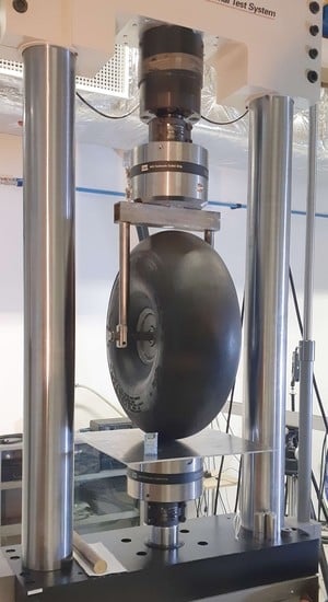
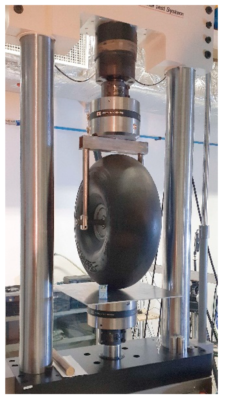
2. Experimental Tests

The tire studied here is a radial 26 in tire, without grooves, used under-inflated for certain types of ground and has a specific structure, different from conventional tires.

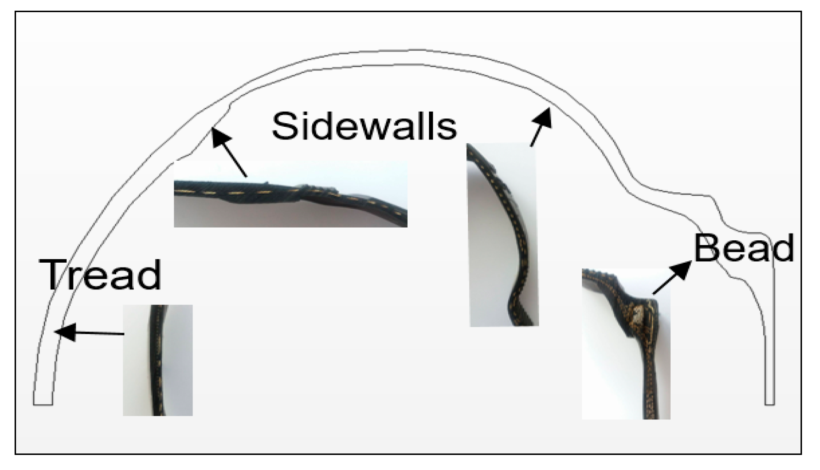
2.1. Cross Section

Experimental investigations were conducted in order to study the inner structure of the tire and to evaluate the material parameters. The tire cross-section was obtained using the water jet cutting technique. This tire showed lower thickness then classic tires. The thickness of the tread is about 6 mm. The thickness of the sidewalls does not exceed 4 mm.

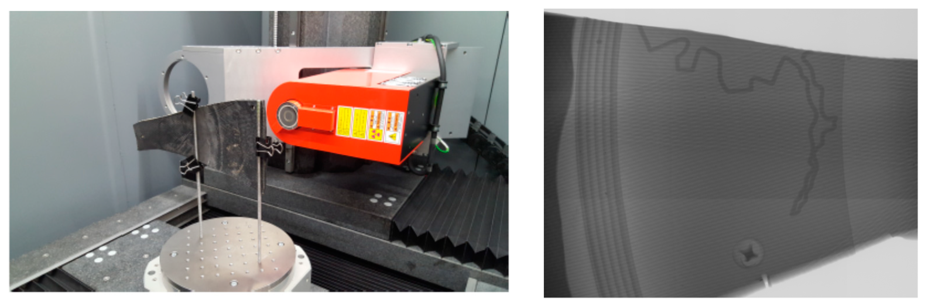
2.2. Inner Structure

The tire is composed of the body, the sidewalls, the beads, and the tread. The body is made of rubberized fabric layers called plies, which give the tire its strength and flexibility. The fabric is made with Kevlar and Nylon fiber. The beads, supporting the rim of the tire, are embedded with steel cords. Different specimen of the reinforced rubber from different parts (tread, side-walls, …) were cut in order to characterize the plies: orientation, spacing between cords, cords diameter, … The different materials of the non-homogeneous areas were separated using custom cut-off tools. Figure 2 presents some of the tire inner structure details in the tire cross-section.

Tomography technology was used to determined the Kevlar and Nylon fiber layers (Figure 3). This technology allowed us to determine with details the reinforcement cords section, spacing, and orientation as mentioned in

Table 1. Reinforcement cords specifications.

Fiber	Section (m2)	Spacing (m)	Orientation (°)
Aramid (Kevlar)	2.46 × 10−8	0.0012	0.0
Nylon	2.45 × 10−7	0.00175	0.0 and 90.0

.

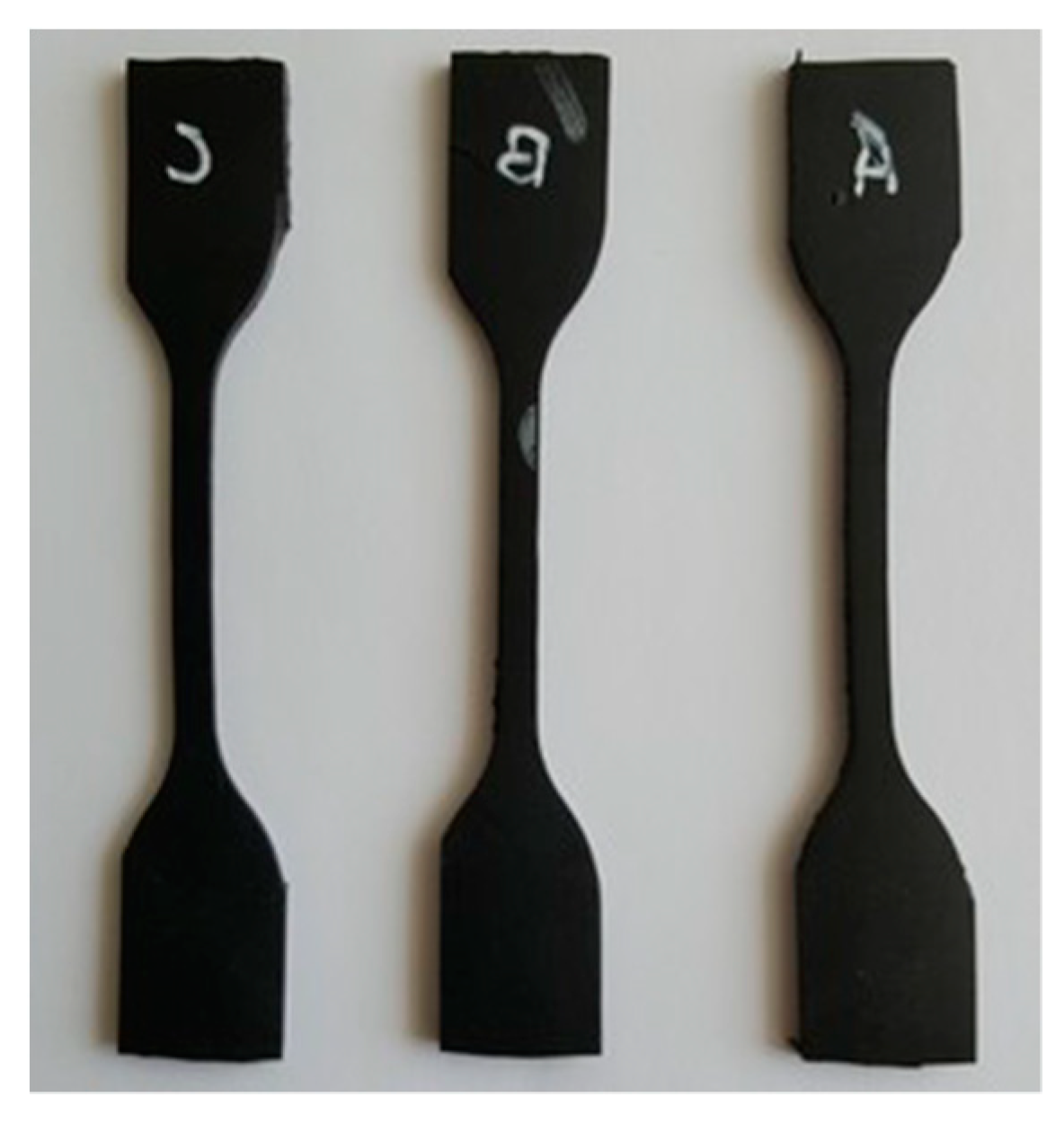
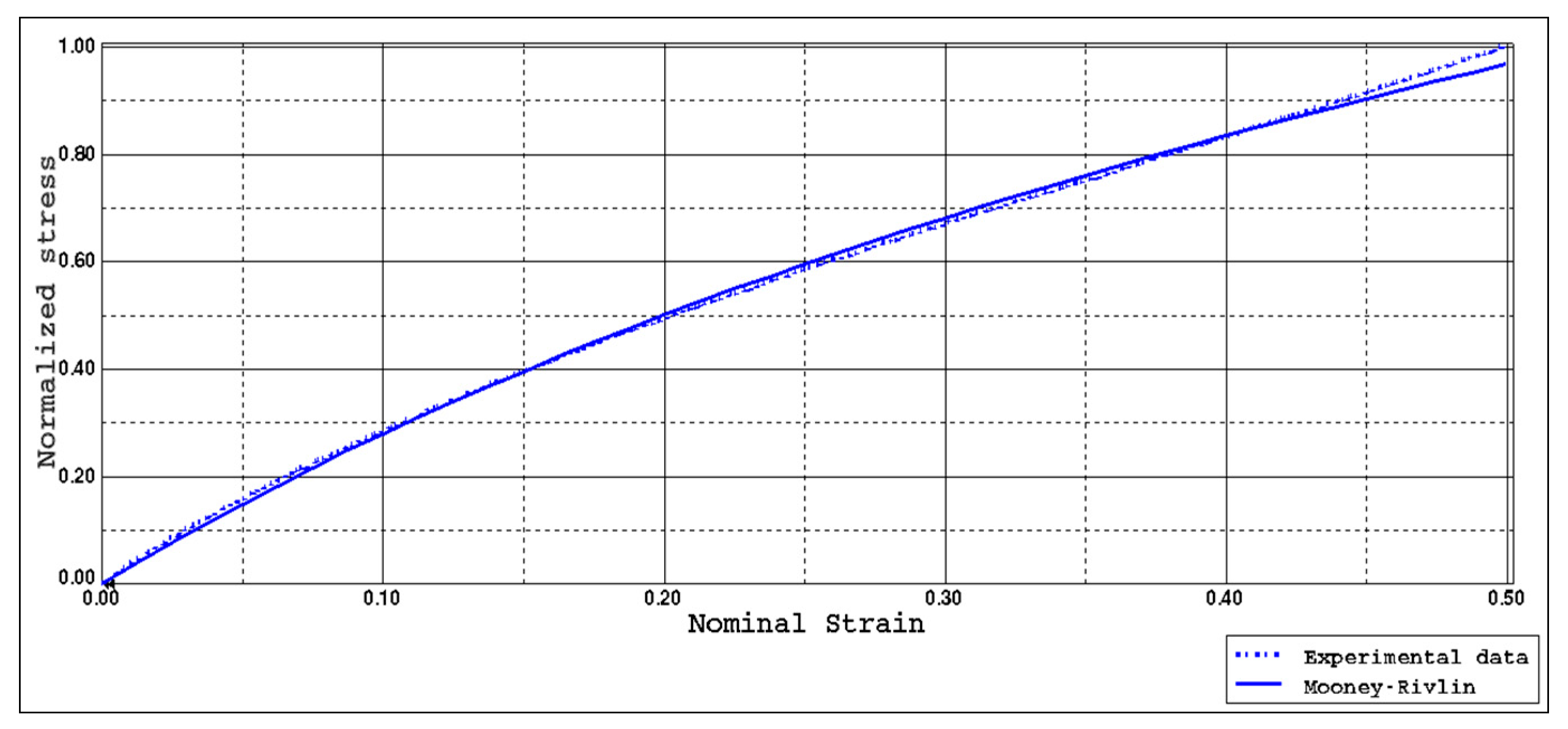
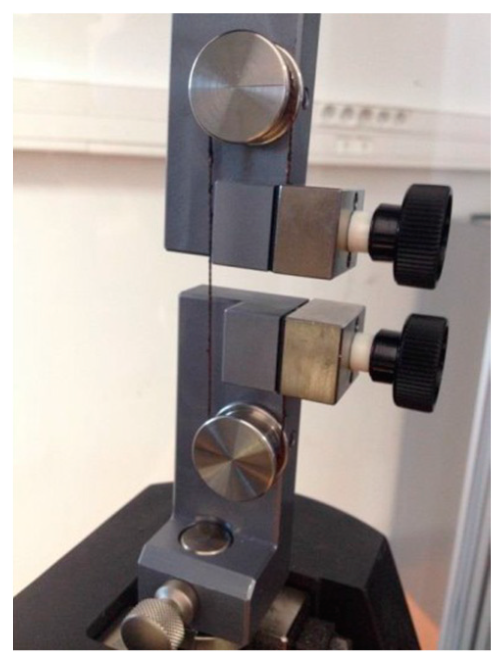
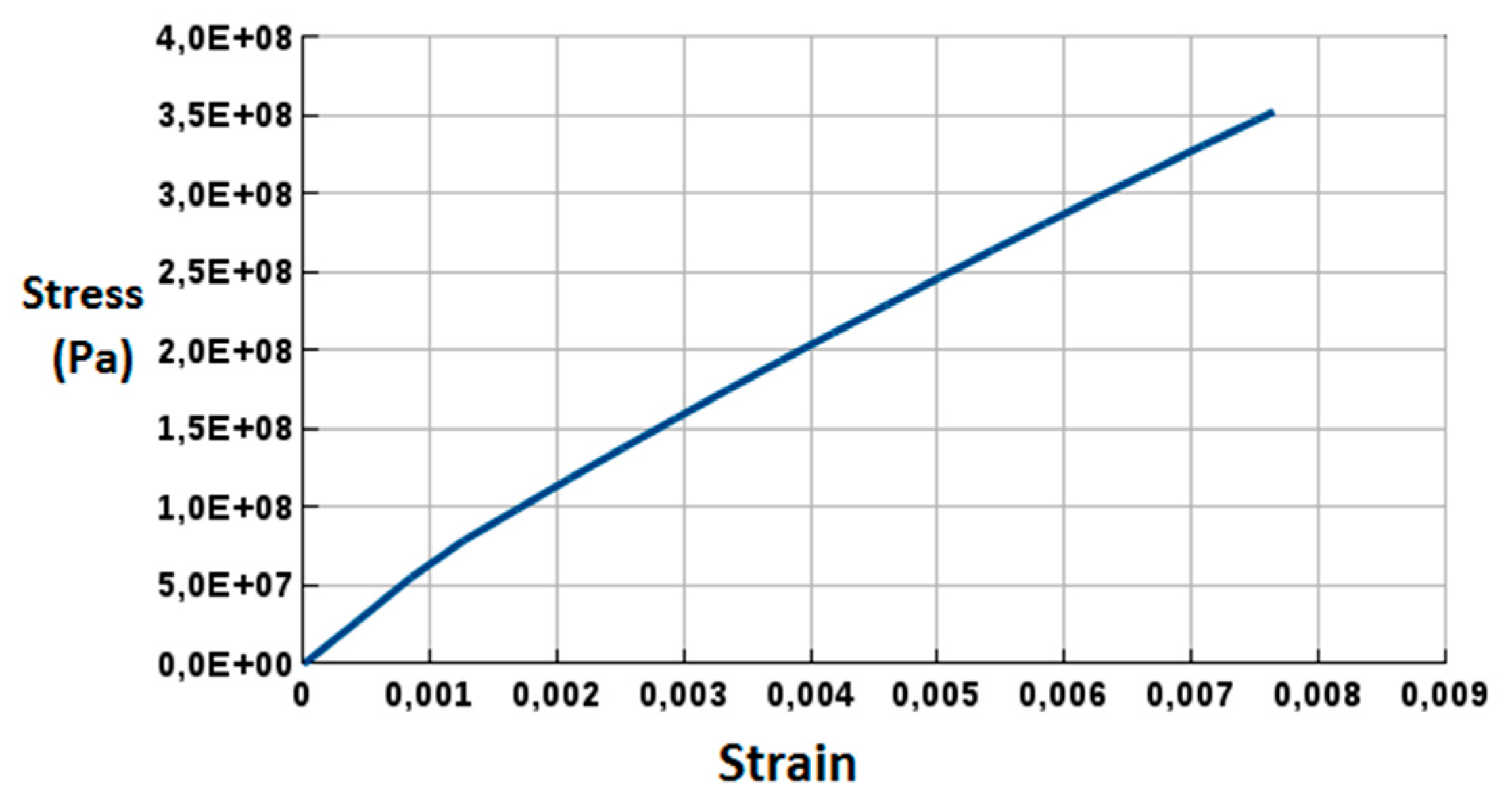
2.3. Materials

The rubber material is considered as hyper-elastic material. Different models are proposed in the literature to describe the non-linear stress–strain relationship of rubbers. Among these models are Arruda-Boyce [13], Ogden et al. [14] and polynomial ones (Neo-Hookean, Yeoh, Mooney-Rivlin) [11]. The hyper-elastic model of Mooney-Rivlin [15] is a polynomial model largely used to describe the tires rubber behavior [5,16]. In this model, the strain energy density function is a linear combination of the two first invariants of the left Cauchy–Green deformation tensor:

$$W=C_{01}\left(I_1-3\right)+C_{02}\left(I_2-3\right)$$

(1)

Mooney-Rivlin model generally suits well the experimental data if the strain level does not reach 30%. Otherwise, the Yeoh model is more appropriate. The rubber specimens were prepared from the tire tread, sidewalls and shoulder (Figure 4).

Figure 5 shows the normalized stress–strain curve obtained. The hyper-elastic model of Mooney–Rivlin predictions matched the experimental test data. The material constants of Mooney–Rivlin law obtained at 20 °C are C₀₁ = 0.3056 MPa and C₀₂ = 0.2134 MPa.

Experimental tests were performed on Kevlar fibers from the carcass. The Figure 6 presents the experimental setup for tensile test of fibers. Figure 7 shows the stress–deformation. The reinforcement cords are described using an elastic model and the Young modulus obtained is 50.8 GPa.

3. Numerical Simulations

The Kongo et al. approach [9,10] concerning the Jumbo-Jet tire was adopted in this study. Experimental investigations are necessary for developing a reliable numerical model of the tire.

3.1. 2D Mesh

In the absence of any CAD tire geometry data, some image acquisition techniques are used to provide the 2D cross-section of tire from the cross-section tire cut. Abaqus code was used to model the final section with clear contours. As shown in the experimental part, the tire is made up of layers of cords embedded in different formulations of rubber. This internal geometric complexity needs to be modelled in order to predict many of the important performance features required from a tire analysis. A typical mesh of the tire cross-section is shown in Figure 8. The reinforcement planes are taken into account in the construction of the 2D model. An embedded 2D axisymmetric mesh model is then obtained. Solid axisymmetric elements are used to mesh the homogeneous rubber (green surfaces in Figure 9) and surface axisymmetric elements are used to mesh the plies (pink and blue lines present the plies planes in Figure 10). Rebars are attached to the surface elements in order to provide the stiffness and the directional response of the cord layers.

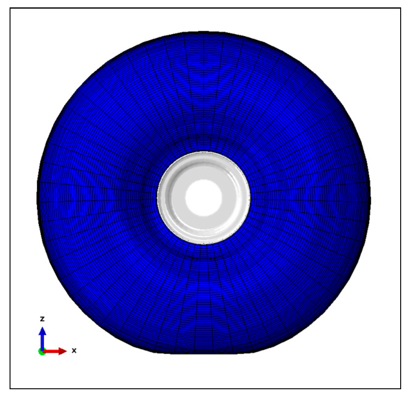
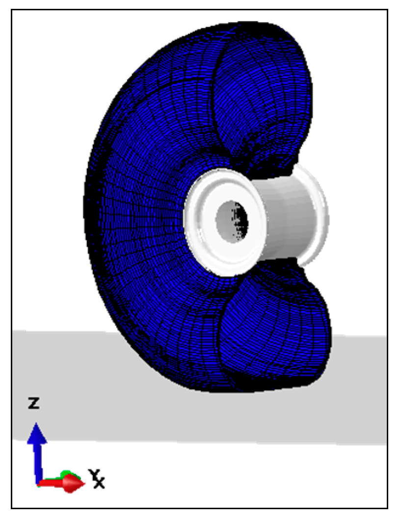
3.2. 3D Mesh

A 3D model was developed by revolving the 2D mesh with 51 parts, as shown in Figure 10. It is considered that the X–Y plane is the runway plane with X the straight rolling direction and Z is the normal vertical loading direction (Figure 11). The rim is modelled using rigid elements. As the contact between rim and tire may not affect the F&M (forces and moments) properties significantly [17], both of them are tied together for convenience and computational efficiency. The nodes at the tire/rim contact are fixed to the rim by a rigid body assumption.

3.3. Simulation Hypothesis

Multiple necessary conditions and different settings are specified:

-

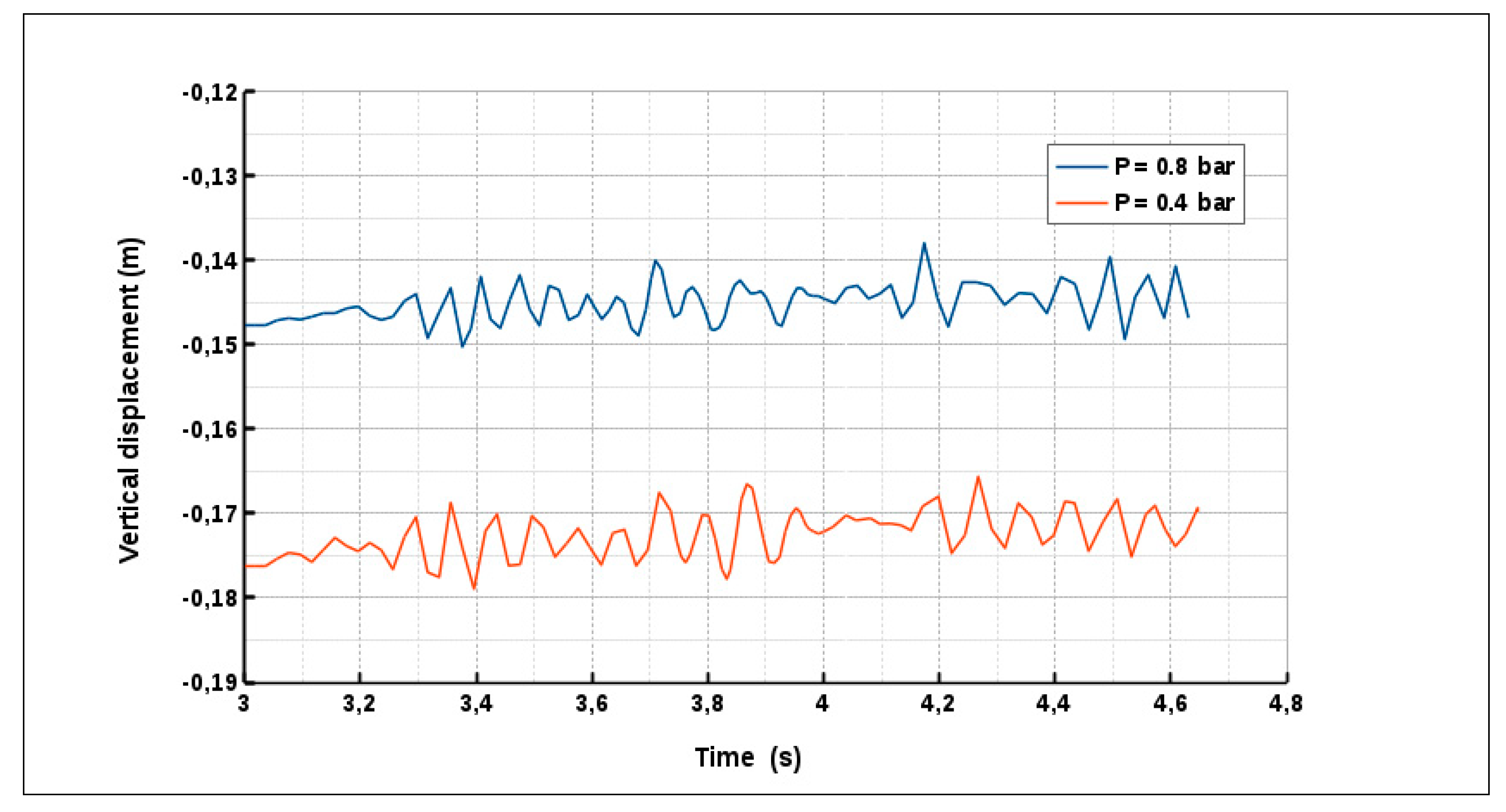
the tire is subjected to a constant inflation pressure according to some specifications (between 0.4 bar and 1.2 bar).

-

a vertical load corresponding to half of the weight of the structure is applied on the rim.

-

the longitudinal displacement/velocity of the tire is applied directly on the rim centre.

-

the runway, considered as a rigid body, is fixed during the simulation.

-

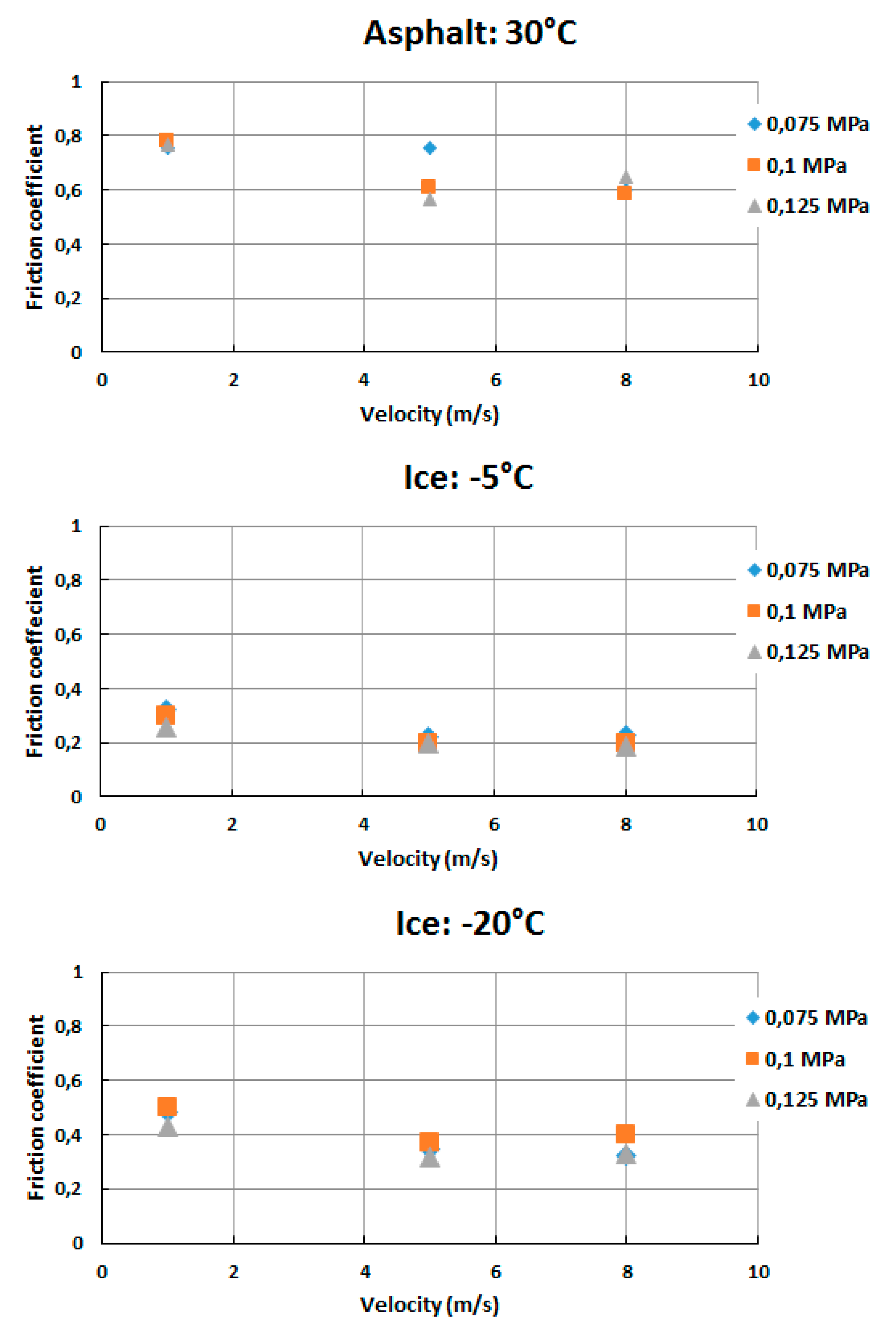
the frictional contact problem in the FEM model is described between a deformable body (tire) and a rigid body (ground). The contact is modelled using non smooth Coulomb and Signorini laws. The friction coefficient is assumed to be constant during one rolling, but different coefficients measured on different surfaces by mean of a tribometer were used.

Bearing in mind that a Bush plane could land on different kinds of grounds, several friction coefficients have been measured on asphalt, ice, clay, or river boulders. Some of these measurements have been done on the HiLiTe friction linear test rig from IDS at Hanover University [18] and some others on a pin-on-disc tribometer in our laboratory.

The Figure 12 present some values of the friction coefficient for asphalt at 30 °C and ice at −5 °C and −20 °C. For river boulders and clay, most of the friction measurements have been done for temperatures ranging from −18 °C to +40 °C.

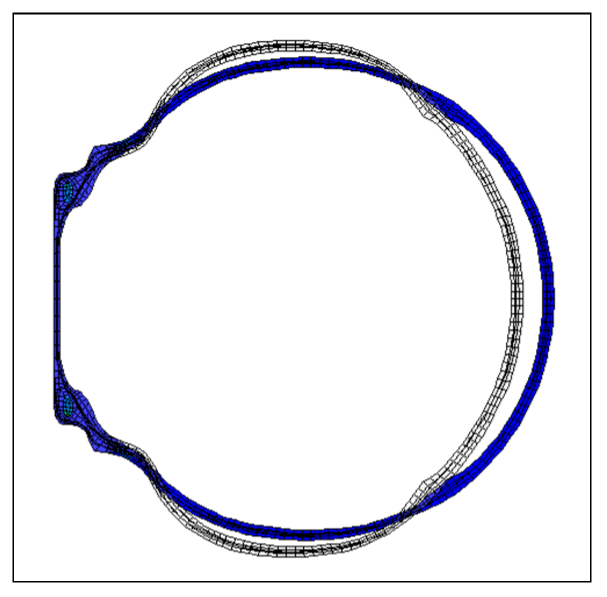
3.4. Model Validation

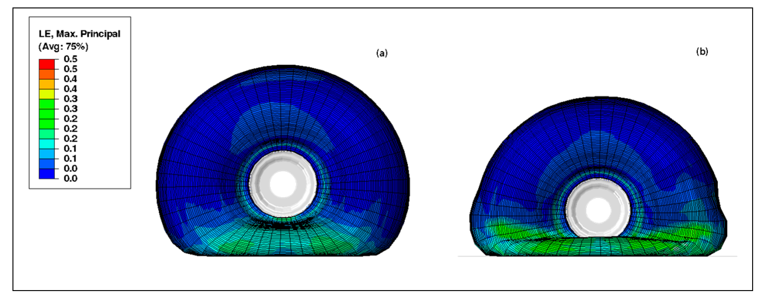
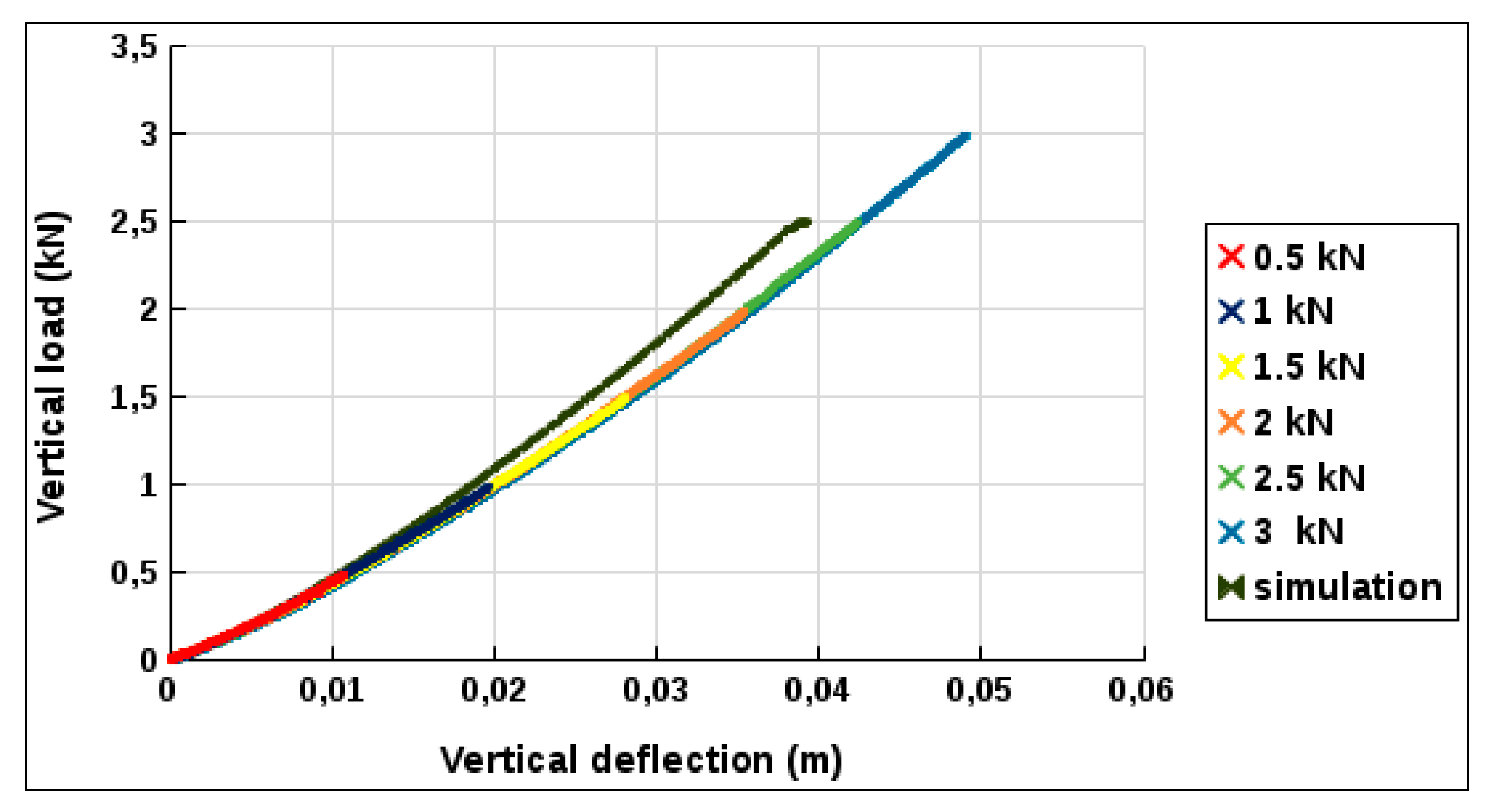
3.4.1. Vertical Loaded Tire

In the validation step, the numerical vertical deflection and the contact area obtained were compared with the experimental results. Using the vertical stiffness measurement test bench (Figure 13), the vertical stiffness of the tire inflated at 0.8 bar is measured at different loads (from 0.5 kN to 3 kN). Figure 14 shows the load–deflection curve obtained numerically in comparison with the experimental results. On one hand, it can be seen from these comparisons that the Bush tire vertical deflection is reproduced through the different measurements. On the other hand, there is a good agreement between the experimental data and the values obtained with the FEM model.

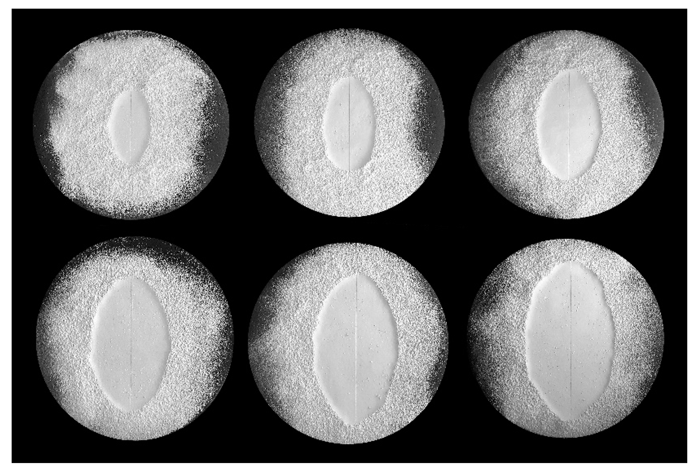
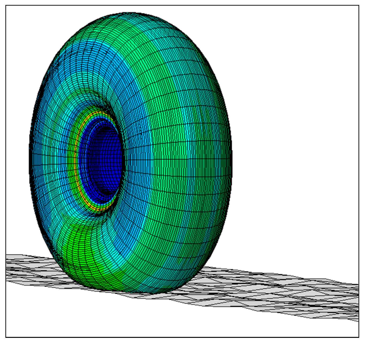
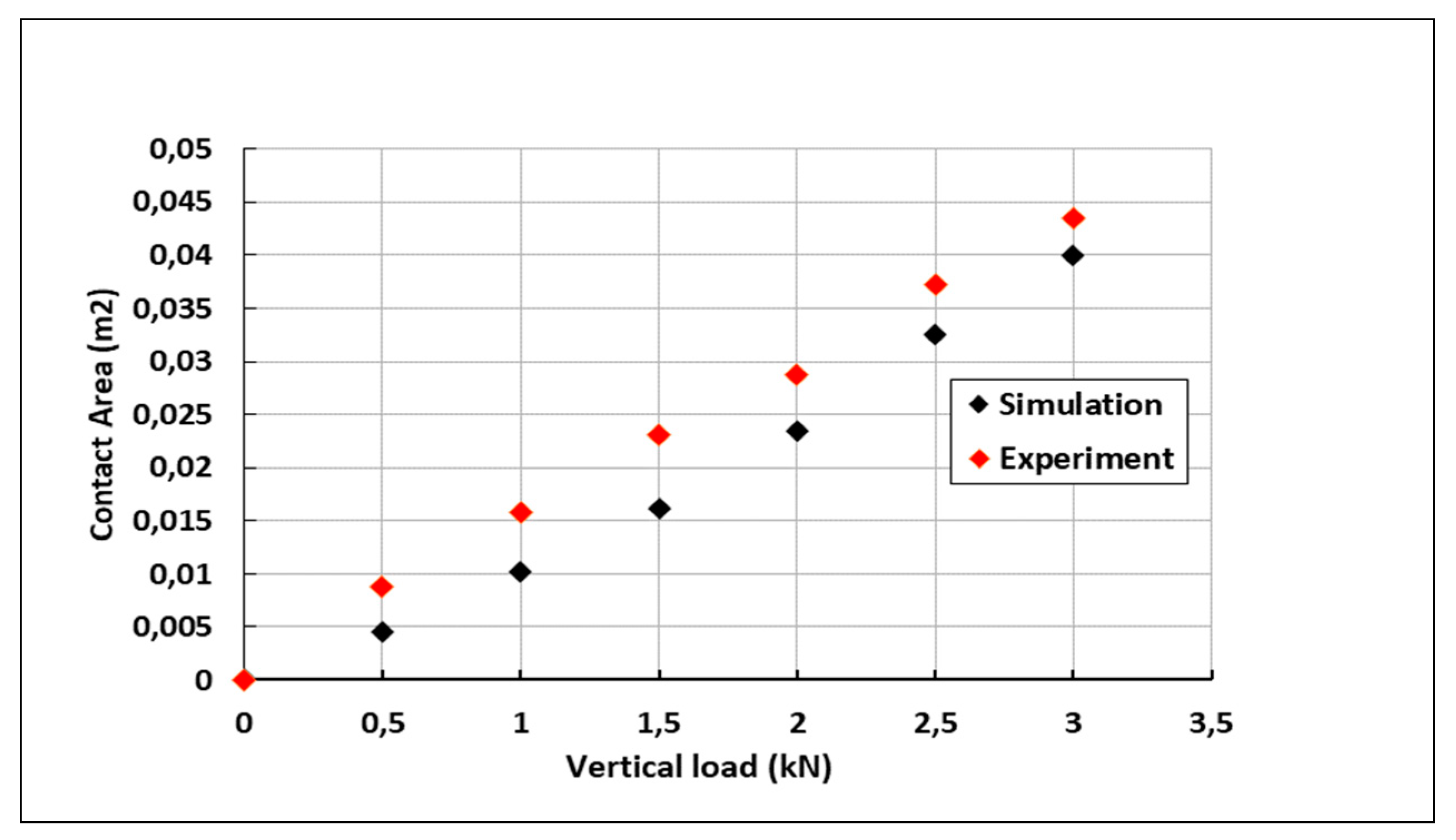
3.4.2. Contact Area

In order to visualize the contact patch, a powder is spread on the contact surface and the surface area of the crushed powder after loading (Figure 15) is measured. Figure 15 shows the evolution of the contact patch of the tire loaded at 0.5, 1, 1.5, 2, 2.5, and 3 kN. The increase of the vertical load leads to an increase of the contact area of the loaded tire. The comparison with the numerical results (Figure 16) shows a good agreement, especially at nominal load.

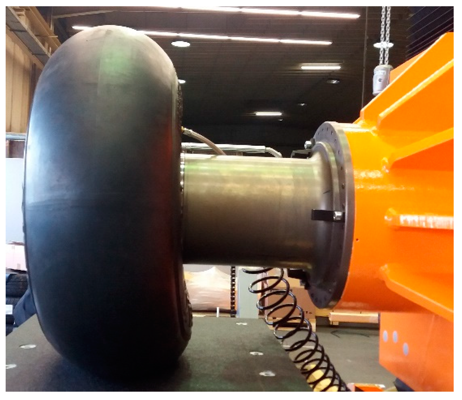
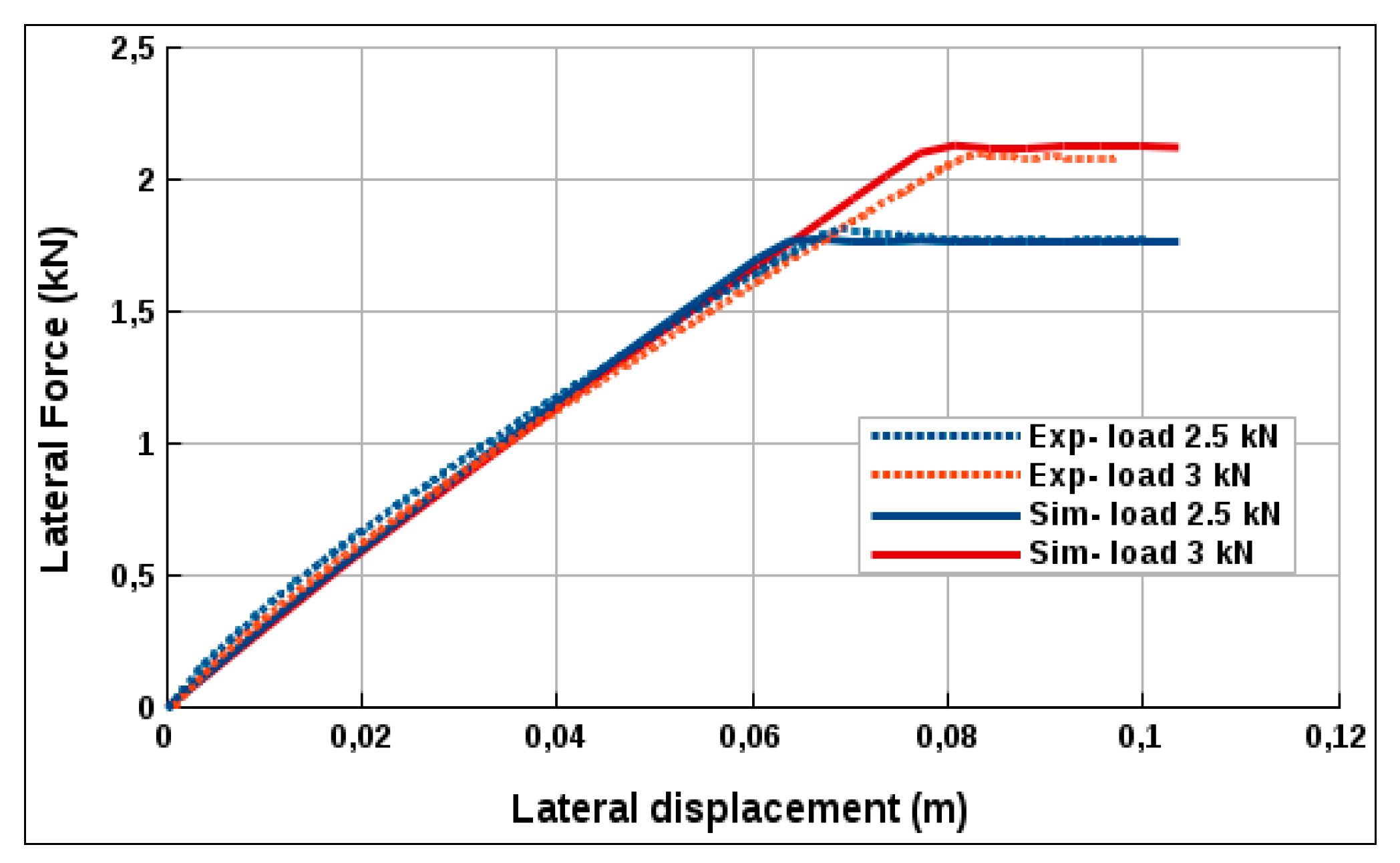
3.4.3. Lateral Loading

For the same reasons as above, we studied the behavior of the Bush tire in lateral loading with the help of the Universal Tire Testing Machine from Testing Systems Company in Aachen, Germany. The experimental setup is presented in Figure 17.

Lateral stiffness measurements were conducted with a tire inflated at 0.8 bar, subjected to two types of vertical loads (Figure 18). The lateral force Fy is plotted as a function of the lateral displacement of the tire center Uy. Each curve has 2 phases: an almost-linearly increasing phase and a flat one that corresponds to the sliding phase where the tangential force is constant at a given vertical load. Numerical results show also great agreement with the experimental data.

4. Dynamic Simulations

4.1. Simulation Steps

The numerical dynamic simulations of tire rolling were conducted in the following manner. First, quasi-static analysis was carried out by inflating the tire and pushing it toward the road surface up to a vertical load of 2.5 kN, which was taken as initial conditions in the transient dynamic analysis. The conditions under which simulation was implemented in each stage are as described in the previous section. Dynamic implicit simulations of the tire rolling are performed within 2 steps:

• acceleration phase: a progressive velocity is applied on the rim to reach a prescribed velocity of 50 kph.
• a steady phase of rolling: a constant velocity of 50 kph along the x-axis is applied on the rim while rolling on different types of runways: flat runway, runway with two successive ramps, and a runway with cleats.

Cornering simulations are also performed:

• acceleration phase: a progressive velocity is applied to reach a prescribed velocity of 50 kph.
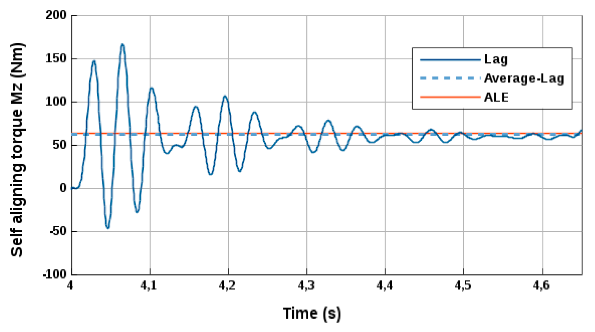
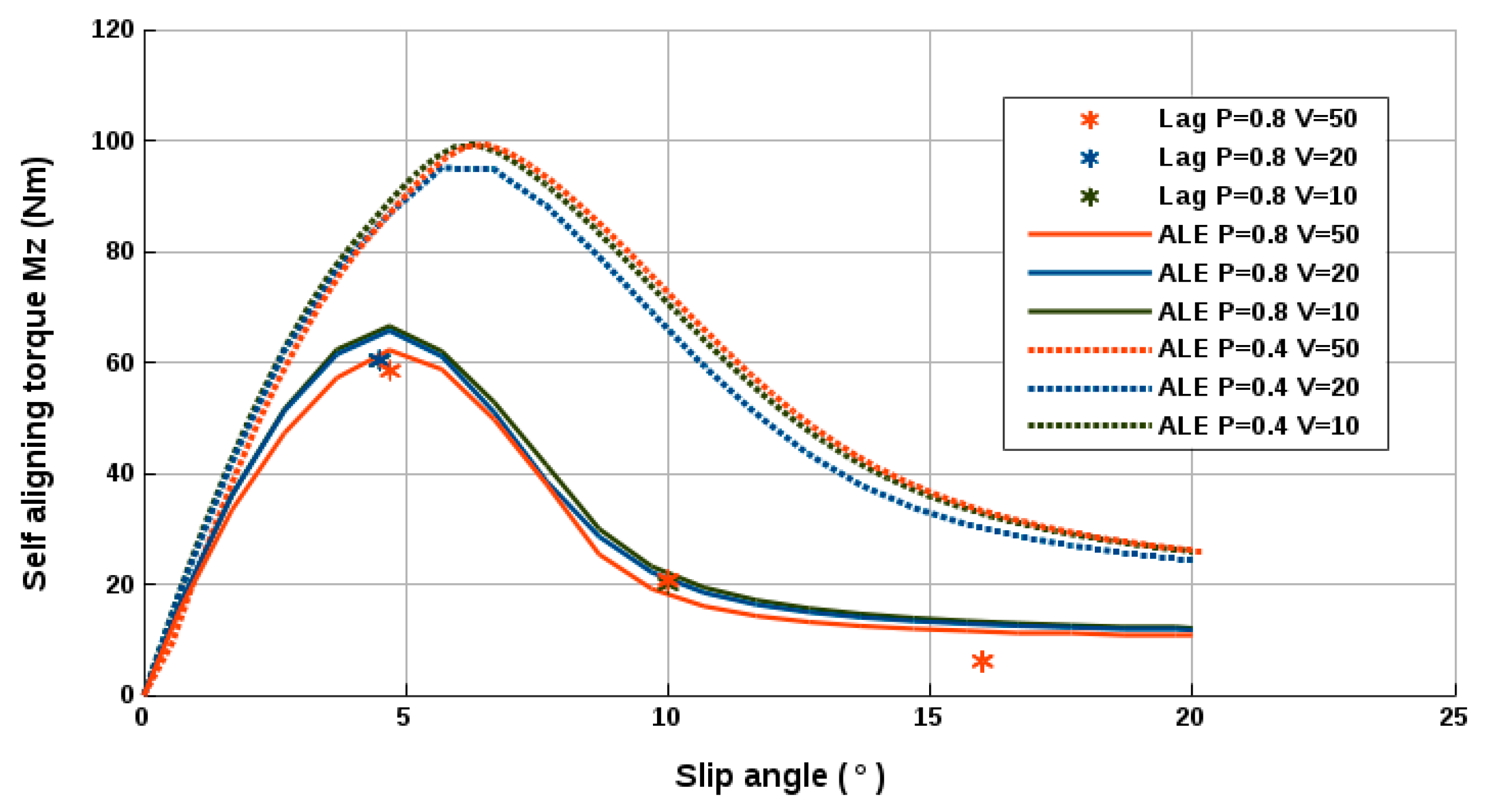
• a steady phase of cornering with constant velocity and slipping angle. By varying the slip angle, cornering simulations allow evaluating the self-aligning moment M_z and the limiting slip angle before the total loss of the adhesion.

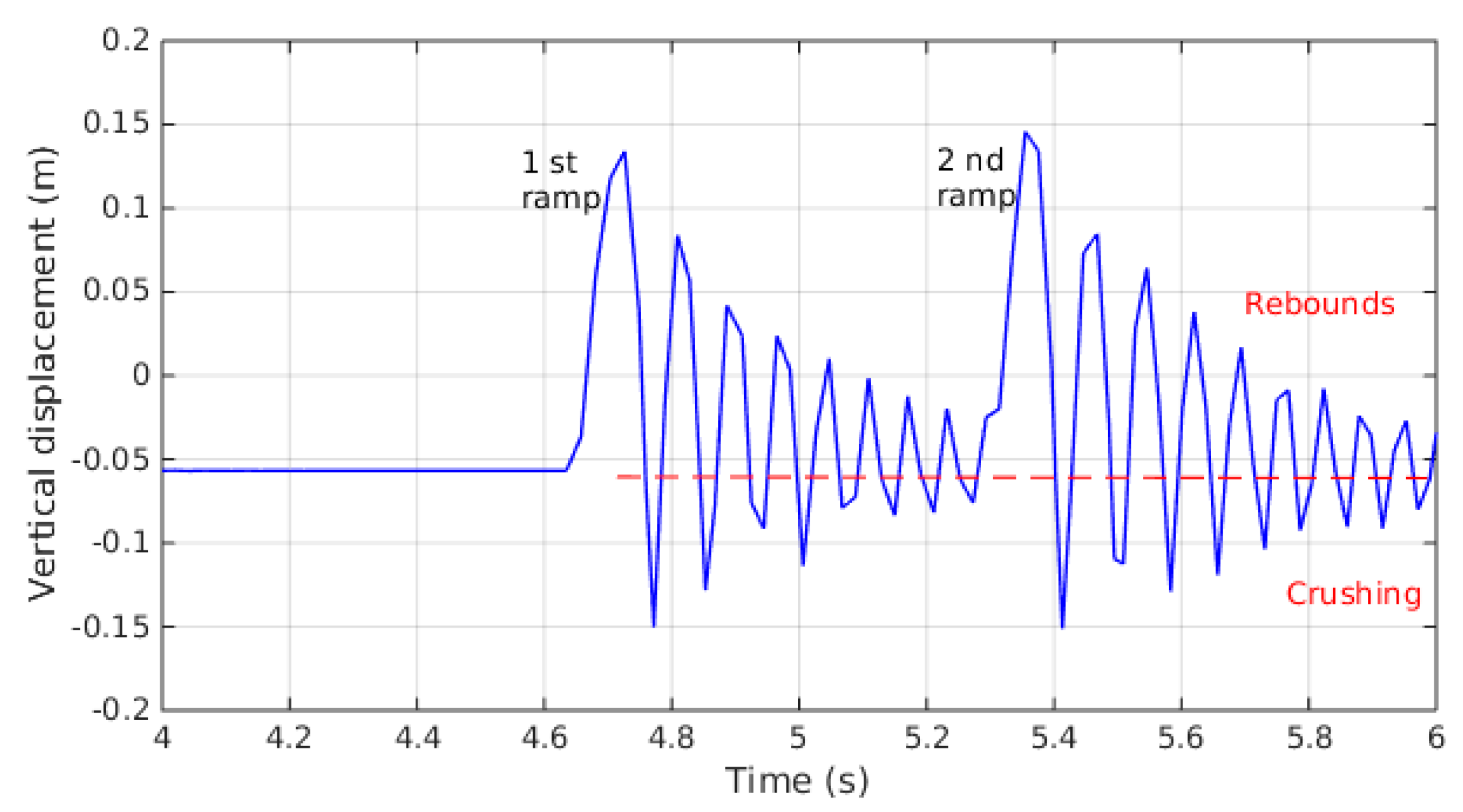
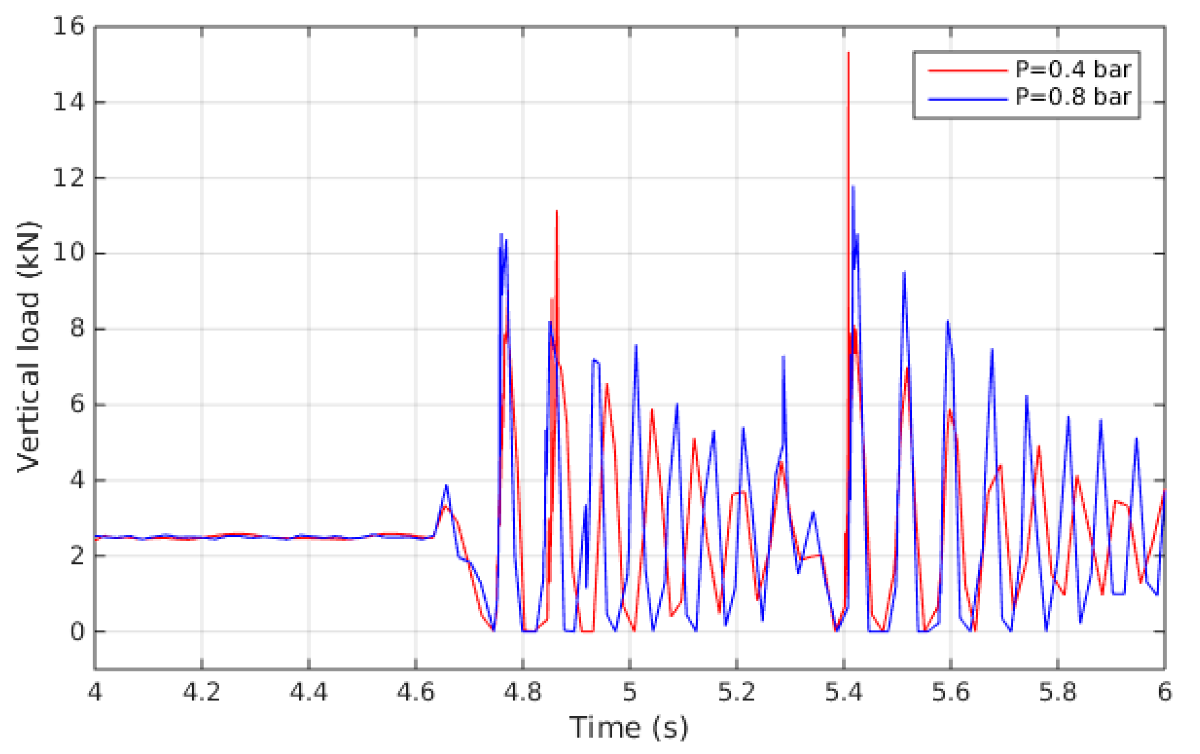
4.2. Rebounds over Ramps

The possible rocks or bumps of the runway are modelled by considering ramps in the ground geometry. Rolling simulations on a runway with two successive ramps of 0.2 m of height are carried out (Figure 19). The first ramp was positioned ahead of the tire to make sure the rolling tire can reach a steady state condition before it reaches the ramp. Figure 20 shows the vertical displacement of the tire. The rebounds during rolling are analyzed. The non-zero initial position indicates the vertical deflection of the tire after loading. The sidewalls of the tire present the most deformed zones with deformation extending from 15% to 30%.

Two cases of inflation pressure P₀ of 0.8 and 0.4 bar respectively are presented. The vertical responses of a rolling tire on a runway with 2 ramps are shown in Figure 21.

The vertical load on the rim during the rolling on a ramp is shown in Figure 21. The vertical load reaches a high value equivalent to 4 times the initial load. It is very important to consider these values while designing the landing gear because this load would be transferred to the frame body. In addition, vertical load shows similar amplitudes in both presented cases, which are in agreement with results shown in Alkan et al. [14]. Rolling over cleats at low velocity was investigated and experiments showed that the inflation pressure does not have any considerable effect on force and moment responses of the tire [8]. On the other hand, the deformations undergone by the tire at the first contact after going beyond the ramp are shown in Figure 22. The results have shown that the pressure of 0.8 bar would be more adequate for runways with large obstacles (~0.2 m). A very low pressure of 0.4 bar would be adapted for runways with sand or mud (Figure 22).

4.3. Rolling over Cleats

Rolling simulations with a velocity of 50 kph on 3D runway with triangular cleats of 0.01 m in height are carried out (Figure 23).

The tread rubber of the tire deforms according to the cleats of the runway. The displacements of the rim during rolling over asperities are shown in Figure 24. Two cases of inflation pressure P₀ of 0.8 and 0.4 bar are presented. The initial gap is due to the difference of the vertical deflection of the inflated tire with two different inflation pressures. The displacements of the tire are almost similar for the two cases. The low pressure did not filter the roughness while rolling under these conditions.

4.4. Cornering

The self-aligning moment M_z is an important characteristic of tires, which directly affects the cornering performance and expresses the ability of a tire to turn back to its steering direction when it is no longer steered. The self-aligning moment (M_z) produces a restoring moment on the tire to realign the direction of travel with the direction of heading when the slip angle is non-zero. Several studies have been carried out on the cornering of vehicle tires [17] and jumbo-jet tires [9,10]. In this study, the response of Bush plane tires in cornering is investigated.

4.4.1. Simulation Approach

Featuring a classical transient dynamic analysis, rolling simulations with cornering are performed. The cornering was obtained by splitting the rolling velocity into longitudinal and lateral components, Vx and Vy. The same rolling steps presented in Section 4.1 are performed. When the classical rolling method obtained from a pure Lagrangian analysis (Lag) is used, only one point is obtained for the chosen loading parameters. As Figure 25 shows, the tire response is time-dependent with this method. It must be noted that several tire rotations are required to reach the stationary phase at which M_z is evaluated.

Thus, a cornering analysis using transient analysis is typically time-consuming. In this application where the detailed transient dynamic behavior is not the primary concern, one can significantly simplify the analysis with the Arbitrary Lagrangian Eulerian (ALE) formulation [7,9,17,19]. The mixed Lagrangian Eulerian computational algorithm is found to be the most efficient and cost-effective tool to simulate steady state behavior [16]. For a rolling body such as a Bush tire, the mesh for ALE analysis deforms but does not rotate in space. In fact, the material flows through the mesh, where a steady-state solution can be obtained for each deformed mesh. An advantage of the non-rotating mesh is that it allows the mesh in the critical region (contact area) to be selectively refined, enhancing simulation efficiency and accuracy. In this case, one simulation is needed to obtain all the M_z values for all the slip angles, while many simulations and much time are required using the classical method (Figure 25).

4.4.2. Simulation Results

Figure 26 shows the self-aligning moment M_z as a function of the slip angle of a tire inflated at different inflation pressures (0.4 bar and 0.8 bar) and rolling with different velocities (10, 20, and 50 kph). The curves mentioned with ALE are obtained with the ALE method. Three cornering simulations with the classical Lagrangian method (Lag) are performed showing the self-aligning moment maximum values and are quite in agreement with the ALE results. Note that the classic shape of a self-aligning moment curve is obtained [9,17,19]. The peak presents the critical slip angle. The effects of inflation pressure variation on M_z are studied. The moment M_z increases by decreasing the inflation pressure. Also, the critical slip angle is greater for smaller inflation pressures. Thus, the tire is increasingly stable by decreasing the inflation pressure, which can be explained by the increase in the contact area. Moreover, the velocity variation has no considerable influence on the self-aligning moment comparing to tire inflation pressure.

5. Conclusions

The present study describes the development of a numerical model for Bush plane tires. The aim of this work is to study the characteristics of this tire in order to predict its rolling behavior on non-regular runways. The different steps of modelling a complicated layered structure, such as aircraft tires, with many plies of rubbers and cords are presented. Also, the tire finite element model is validated through experimental static tests (vertical and lateral loading). The tire rolling behavior is studied through three steps. Simulations of rolling over small cleats were conducted, and it was shown that low pressure did not dampen the roughness while rolling under these conditions. Furthermore, simulations of rolling over ramps were presented. Tires have been deformed and undergone multiple rebounds due to the shocks. Analyzing rebounds is a critical step for studying Bush plane landing gears [20]. Finally, the tire self-aligning moment was studied with ALE analysis and the critical slip angle was determined. The inflation pressure influence and the velocity influence on the self-aligning moment were highlighted.

References

- Bush Plane. Available online: http://www.micheljulien.com (accessed on 1 January 2018).
- Bush Tire. Available online: http://www.beringer-aero.com (accessed on 1 January 2018).
- Pacejka, H.B.; Bakker, E. The magic formula tyre model. Veh. Syst. Dyn. 1993, 21, 1–18. [Google Scholar] [CrossRef]
- Besselink, I.J.M.; Schmeitz, A.J.C.; Pacejka, H.B. An improved Magic Formula/Swift tyre model that can handle inflation pressure changes. Veh. Syst. Dyn. 2010, 48, 337–352. [Google Scholar] [CrossRef]
- Faria, L.O.; Bass, J.M.; Oden, J.T.; Becker, E.B. A Three-Dimensional Rolling Contact Model for a Reinforced Rubber Tire. Tire Sci. Technol. 1989, 17, 217–233. [Google Scholar] [CrossRef]
- Chongfeng, W.; Oluremi, A.O. Transient dynamic behaviour of finite element tire traversing obstacles with different heights. J. Terramech. 2014, 56, 1–16. [Google Scholar]
- Palanivelu, S.; Rao, K.V.; Kumar, R.K. Determination of rolling tyre modal parameters using Finite Element techniques and Operational Modal Analysis. Mech. Syst. Signal Process. 2015, 64–65, 385–402. [Google Scholar] [CrossRef]
- Alkan, V.; Karamihas, S.M. Experimental analysis of tire-enveloping characteristics at low velocity. Veh. Syst. Dyn. 2009, 47, 575–587. [Google Scholar] [CrossRef]
- Kondé, A.K.; Rosu, I.; Lebon, F.; Brardo, O.; Devésa, B. Thermo-Mechanical analysis of an aircraft tire in cornering using coupled ALE and Lagrangian formulation. Cent. Eur. J. Eng. 2012, 3, 191–205. [Google Scholar]
- Kondé, A.K.; Rosu, I.; Lebon, F.; Brardo, O.; Devésa, B. On the modeling of aircraft tire. Aerosp. Sci. Technol. 2013, 27, 67–75. [Google Scholar] [CrossRef]
- Behroozi, M.; Olatunbosun, O.A.; Ding, W. Finite element analysis of aircraft tyre—Effect of model complexity on tyre performance characteristics. Mater. Des. 2012, 35, 810–819. [Google Scholar] [CrossRef]
- The 3DEXPERIENCE Company. Rebar modeling in shell, membrane, and surface elements. In Abaqus Theory Guide; The 3DEXPERIENCE Company: Vélizy-Villacoublay, France, 2014. [Google Scholar]
- Boyce, M.C.; Arruda, E.M. Constitutive models of rubber elasticity. Rubber Chem. Technol. 2000, 73, 504–523. [Google Scholar] [CrossRef]
- Ogden, R.W.; Saccomandi, G.; Sgura, I. Fitting hyperelastic models to experimental data. Comput. Mech. 2004, 34, 484–502. [Google Scholar] [CrossRef]
- Rivlin, R.S.; Saunders, D.W. Large elastic deformations of isotropic materials VII. Experiments on the deformation of rubber. Philos. Trans. R. Soc. Lond. Ser. A 1995, 2243, 251–288. [Google Scholar] [CrossRef]
- Crudu, M. Étude Expérimentale et Numérique des Joints Hydrauliques. Ph.D. Thesis, University of Poitiers, Poitiers, France, 2012. [Google Scholar]
- Rao, K.V.N.; Kumar, R.K. Simulation of Tire Dynamic Behavior Using Various Finite Element Techniques. Int. J. Comput. Methods Eng. Sci. Mech. 2007, 8, 363–372. [Google Scholar]
- Linke, T.; Wangenheim, M.; Lind, H.; Ripka, S. Experimental Friction and Temperature Investigation on Aircraft Tires. Tire Sci. Technol. 2014, 42, 116–144. [Google Scholar]
- Nackenhorst, U. The ALE-formulation of bodies in rolling contact—Theoretical foundations and finite element approach. Comput. Methods Appl. Mech. Eng. 2004, 193, 4299–4322. [Google Scholar] [CrossRef]
- Arif, N.; Rosu, I.; Lebon, F.; Elias-Birembaux, H. On the Modeling of Light Aircraft Landing Gears. J. Aeronaut. Aerosp. Eng. 2018, 7, 3. [Google Scholar]