Article

Thermal Turbulent Flow in Leading Edge Grooved and Conventional Tilting Pad Journal Bearing Segments—A Comparative Study

Division of Machine Elements, Luleå University of Technology, 971 87 Luleå, Sweden
*
Author to whom correspondence should be addressed.
Lubricants 2018, 6(4), 97; https://doi.org/10.3390/lubricants6040097
Submission received: 1 August 2018 / Revised: 16 October 2018 / Accepted: 24 October 2018 / Published: 2 November 2018
(This article belongs to the Special Issue Multiphysics and Multiscale Models of Tribology)

Abstract

:
A comparative study between a conventional- and leading edge grooved (LEG) tilting pad journal bearing (TPJB) segment is performed. The developed model uses the Shear Stress Transport (SST) turbulence model, coupled with the energy equation and a partial differential equation for the fluid domain mesh displacement to predict the thermal flow characteristics. Instead of using an effective boundary condition to determine the inlet temperature of the LEG pad and excluding the additional LEG portion, as is common practice, the whole geometry of the LEG is modeled. Several sizes of the LEG portion is investigated and it is shown to have quite a small influence on pressure, temperature, film thickness and turbulence intensity. Moreover, the results also show that the conventional pad gives rise to higher levels of turbulence in the mid plane compared to its LEG counterpart, while the latter has a marginally higher value of turbulence when the volume average value is computed. The maximum value of turbulence is however present in the conventional model.

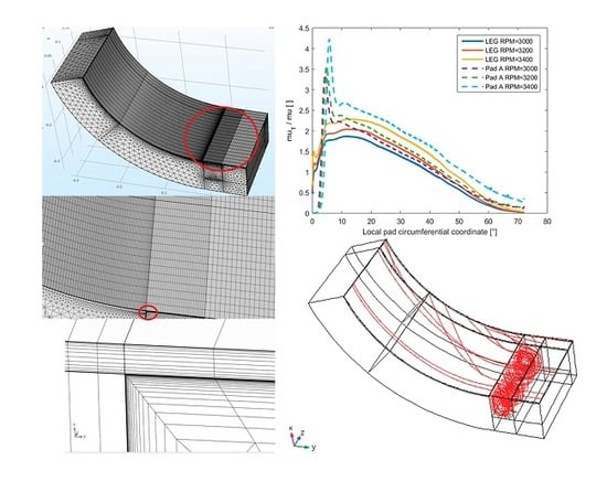
Graphical Abstract

1. Introduction

The leading edge groove (LEG) design has been proven more effective in reducing temperature and power losses in tilting pad thrust bearings in comparison to other methods of lubrication, as shown in e.g., Mikula et al. [1,2]. Studies on the benefits of an LEG in tilting pad journal bearings (TPJBs) has, however, been less conclusive. See, for example, [3,4]. Though generally speaking, it seems to be the consensus that the LEG TPJB operates under lower metal temperatures and power losses than its conventional counterpart. When it comes to modeling the LEG TPJB, it has traditionally been done by assuming an effective mixing model for the inlet temperature at each pad. See, for example, [5,6]. He et al. [7] also considered different profiles across the film thickness for their inlet temperature but could not match their experimental data until they lowered their transitional Reynolds number for turbulence in their model, implying that the LEG introduces a disturbance to the flow which causes an onset of turbulence to occur. Very few studies can be found where the actual geometry of the LEG has been modeled and they are either in 2D or do not involve any turbulence model, e.g., [8,9]. The latter article did, however, present an interesting work on controllable (“smart”) lubrication in an LEG TPJB. While the study of turbulence in journal bearings typically uses classic thin film theory, see e.g., [10,11,12,13], more advanced models are now being implemented as Computational Fluid Dynamics (CFD) becomes more of a mainstream tool, see e.g., [14,15]. Armentrout et al. [16] performed a comparison between a classic thin film turbulence model with a Shear Stress Transport ( k ω ) model in a water lubricated TPJB. The results showed an initial discrepancy which was reduced as the model constants for the simpler model were updated and the grid refined in the radial direction. They did, however, not take any temperature effects into account. Furthermore, there exist several experimental studies on large TPJBs, similar in size to the one considered in this article, see e.g., [17,18], where the results in the latter article indicated that turbulence effects need to be considered at a rotational speed of around 2500 rpm for a moderate load. With this background, the current work is a first step towards assessing whether or not modeling the actual geometry of an LEG portion gives rise to any significant discrepancies between results when compared to the traditional way of modeling the LEG, i.e., with an effective temperature boundary condition at the inlet and ignoring the additional geometry that is the LEG portion. To simplify the analysis, no deformations of the surrounding solids are included, although they have been shown to play a significant role in the performance of bearings [17,19]. More specifically, the work in this article also seeks out to answer the notion of triggered turbulence from [7]. Generally, high levels of turbulence in a bearing is something that is unwanted due to the increase of friction power losses. A successful, realistic, model of an LEG would also be useful in terms of being able to perform any meaningful shape optimization of the LEG geometry. To the author’s best knowledge, the model presented in this work represents the state of the art when it comes to multi physics modeling of an LEG TPJB.

2. Geometry

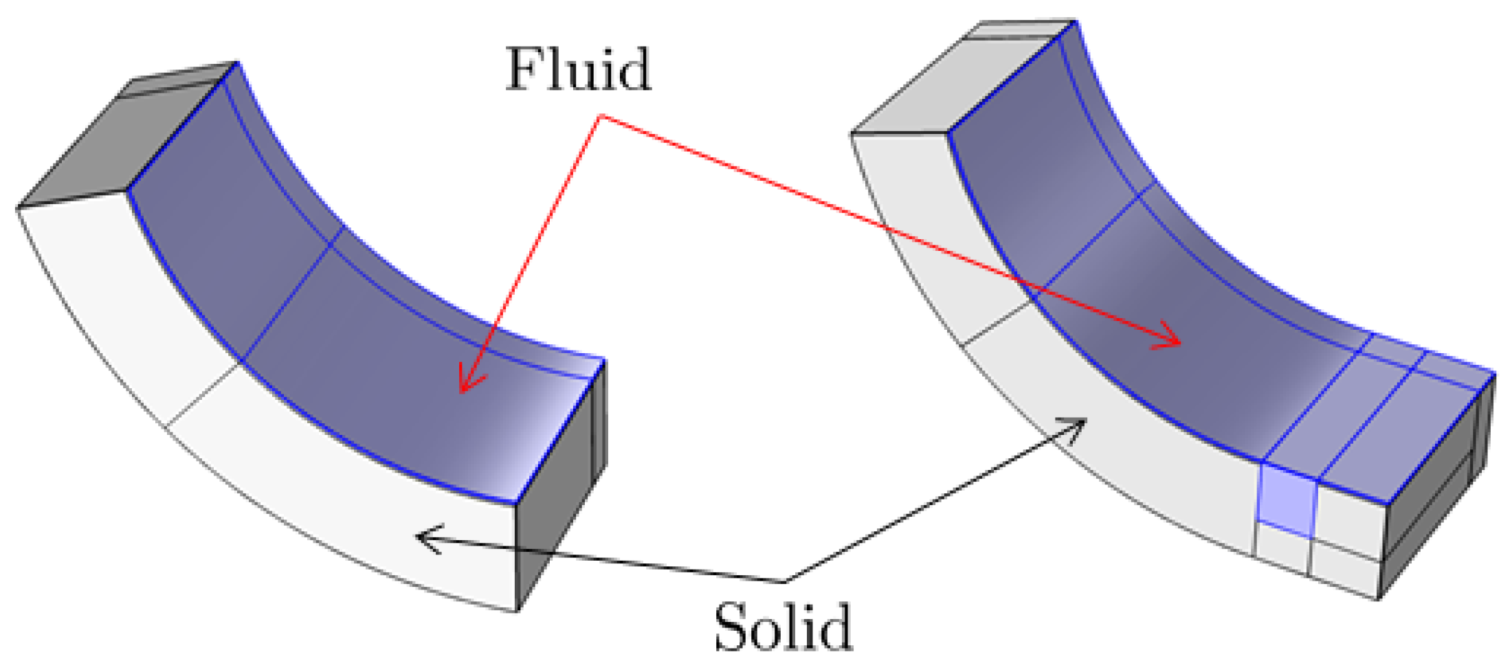
Two different concepts, or geometries, are investigated and compared in this study. The first geometry concept is referred to as “Pad A” and the second one “Pad B”, they represent the conventional- and LEG pad design respectively, as is illustrated in Figure 1. Note the inlet hole in the LEG of Pad B, marked with blue color.
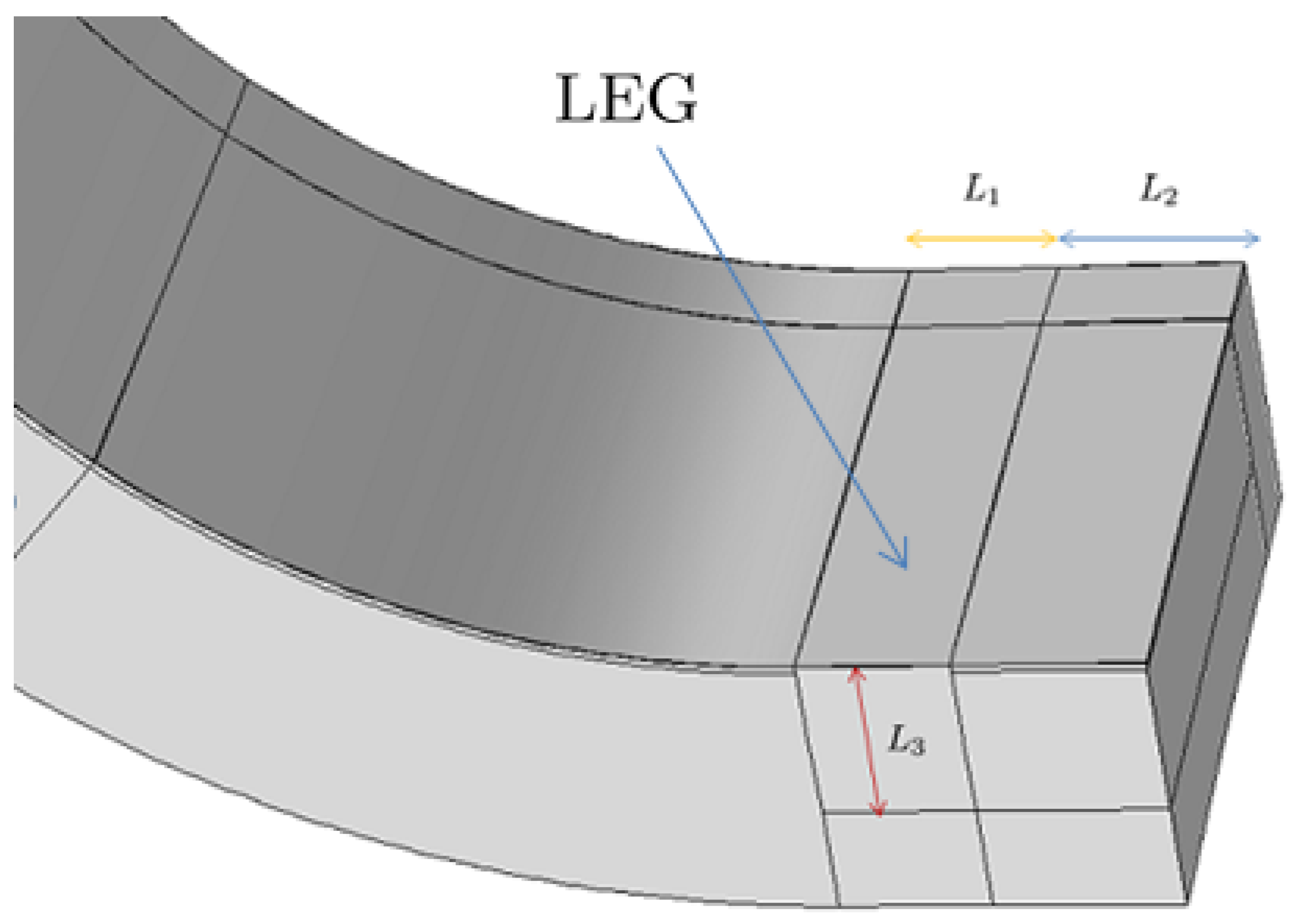
Note that, in Figure 1, only half of the axial length is modeled due to symmetry reasons. The two pads are of the exact same size and the only thing separating them, geometrically speaking, is the additional LEG portion seen on Pad B. Throughout this article, the term “LEG portion” will refer to the total geometry of the LEG and the small pad section that precedes it. For extra clarity, Figure 2 shows the fluid and solid domains of the pads highlighted in blue and gray, respectively, while the additional geometry of the LEG portion is further illustrated in Figure 3.
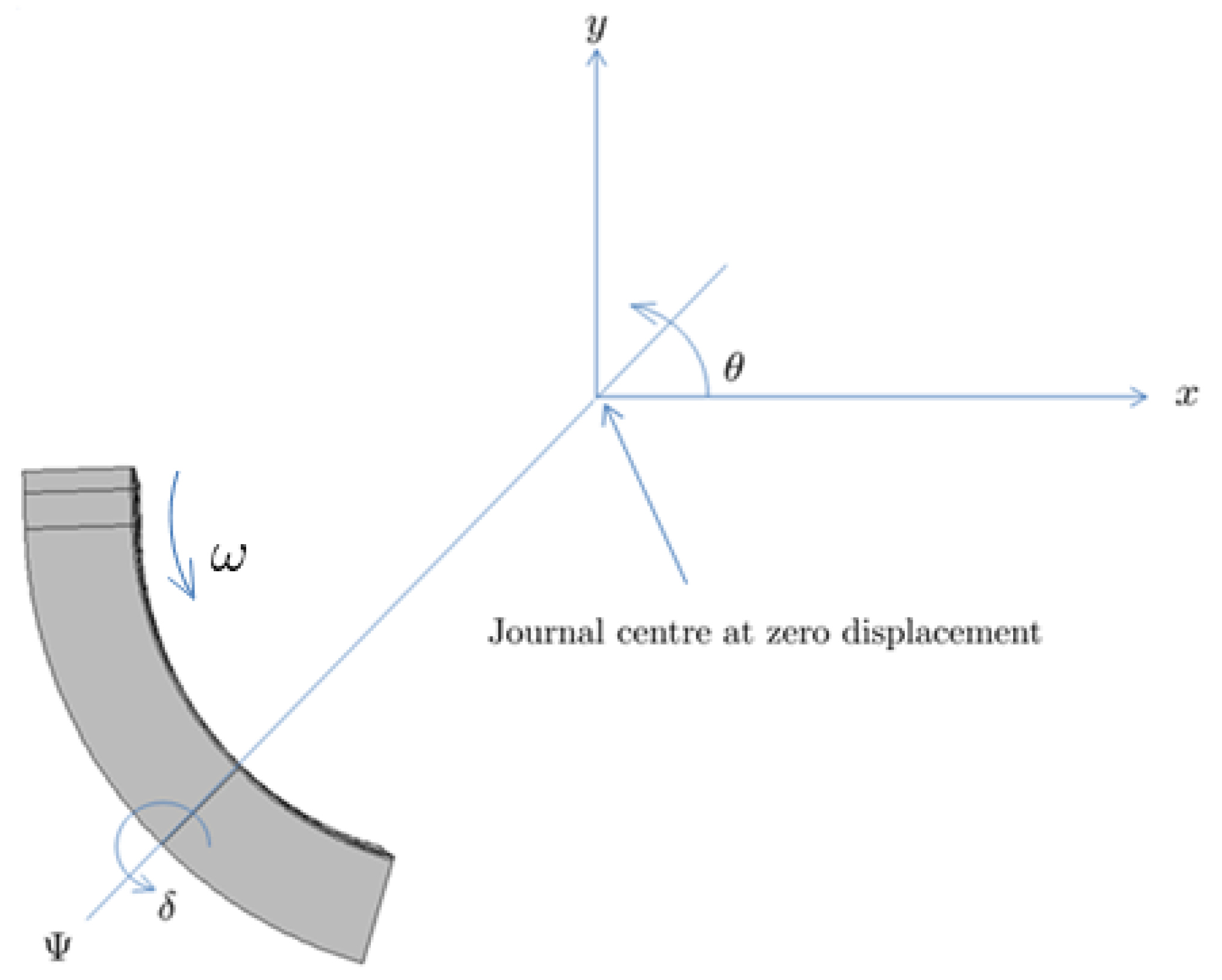
The spatial position and orientation of the pad with respect to a right-handed x y z coordinate system is shown in Figure 4. Moreover, the LEG portion does not follow the pad radius of curvature but is simply an extrusion normal to its adjacent pad surface. Although this was done to simplify the geometry and the corresponding meshing, it is still not an un-realistic design since some LEG pads are manufactured in this manner.

3. Model

All of the equations presented below are in their steady state form for an incompressible fluid. The only material parameter that is assumed non constant, but changes with temperature, is the molecular dynamic viscosity μ . As for the geometry, the shaft eccentricity is fixed throughout the simulations. A schematic 2D view of the pad geometry is illustrated in Figure 1. Moreover, all equations presented in this article are solved using the FE software COMSOL Multiphysics.

3.1. Fluid Dynamics

The characteristics of the flow are governed by the Reynolds Averaged Navier Stokes (RANS) Shear Stress Transport (SST) turbulence model [20,21]. This model combines the free stream predictions of the k ε -model with the robust near wall predictions of the k ω -model. Moreover, it is based on the eddy viscosity concept and uses, apart from the RANS equations, two additional PDE:s for k and ω to calculate this turbulent (eddy) viscosity. The main equations of the model are given below:
ρ U ¯ · U ¯ + · ( ρ u u ¯ ) = P + · μ ( U ¯ + ( U ¯ ) T ,
ρ U ¯ = 0 ,
( ρ u u ¯ ) = μ T ( U ¯ + ( U ¯ ) T ) + 2 3 ρ k ,
μ T = ρ a 1 k max ( a 1 ω , S f v 2 ) ,
ρ U ¯ · k = P ρ β 0 k ω + · ( ( μ + σ k μ T ) k ) ,
ρ U ¯ · ω = ρ γ μ T P ρ β ω 2 + · ( ( μ + σ ω μ T ) ω ) + 2 ( 1 f v 1 ) ρ σ ω 2 ω ω · k .
In Equations (3)–(6), U ¯ is the temporal mean velocity vector, u is the turbulent velocity fluctuation vector, k and ω are the turbulent kinetic energy and specific dissipation rate respectively, ρ is the fluid density and μ T is the dynamic turbulent viscosity. Furthermore, P is the turbulent production term, S = S i j S i j is a characteristic magnitude of the mean rate of strain tensor S ¯ , f v 1 , f v 2 are interpolation functions and a 1 , β 0 , σ k , σ ω 2 , σ ω , β , γ are model constants. More details on the model can be found in the references given above. Furthermore, no cavitation model was considered in this work since only positive pressures were encountered.

3.2. Thermal Equations

The temporal mean temperature in the fluid film is governed by the Reynolds Averaged energy equation of the following form (see e.g., [22])
ρ C p U ¯ · T ¯ = · ( ( λ + λ T ) T ¯ ) + τ ¯ : S ¯ ,
λ T = μ T C p Pr T ,
Pr T = ( 1 2 Pr T + 0.3 C p μ T Pr T λ ( 0.3 C p μ T λ ) 2 ( 1 exp ( λ 0.3 C p μ T Pr T ) ) ) 1 .
In Equations (8) and (9), T ¯ is the temporal mean temperature, C p is the specific heat capacity, λ , λ T are the laminar and turbulent heat conductivity, respectively, τ ¯ is the viscous stress tensor based on the mean rate of strain tensor S ¯ , Pr T is the turbulent Prandtl number and Pr T is the turbulent Prandtl number in the far field, see [23], with Pr T = 0.85 . The molecular viscosity-temperature dependence in the fluid is modeled by the Vogel equation:
μ ( T ) = A exp ( B T C ) .
Moreover, the heat conduction in the solids is governed by the classic Laplace equation:
λ s 2 T = 0 ,
where λ s is the heat conductivity in the solid materials.

3.3. Dynamic Meshing

Since the pad is free to rotate around its pivot, the fluid domain will deform as a function of the tilt angle δ . This deformation is taken care of by using the Moving mesh interface in COMSOL. The shape of the fluid domain is completely determined by the film thickness which is given by
h ( θ ) = C p ˜ + ( C p ˜ C b ˜ ) cos ( θ Ψ ) e x cos ( θ ) e y sin ( θ ) ( R a + d ) δ sin ( θ Ψ ) ,
where C p ˜ , C b ˜ are the radial pad- and bearing clearances, respectively, d is the pad thickness, R a is the journal radius and e x , e y are the journal x and y eccentricities, respectively. Moreover, Ψ is the angular position of the pivot (see Figure 4). This film thickness is imposed in COMSOL by adding a mesh displacement equal to d 0 + h ( θ ) in the normal direction to the pad surface on the top surface of the fluid domain (fluid–shaft interface). The parameter d 0 is arbitrary but should be of the same order as h. It represents the (constant) film thickness of the original geometry. To find the tilt angle δ , an equation for the moment balance around the pivot is added to the set of governing equations, it has the form
A p · ( d + R a ) sin ( θ Ψ ) d A = 0 ,
where p is the hydrodynamic pressure and A is the surface area of the fluid domain. Note that, in Equation (13), no contribution from viscous forces has been included. Moreover, to deform the mesh inside the boundaries with prescribed displacement, the Yeoh smoothing method was used with a stiffening factor of 100 (see, e.g., [24]).

3.4. Boundary Conditions

The terminology used here for the boundary conditions is the one that COMSOL Multiphysics uses. For more information, the reader is referred to [24]. For all the physics, the axial symmetry in the model was ensured by using a condition of zero gradient in the direction normal to the symmetry plane.

3.4.1. Fluid Flow

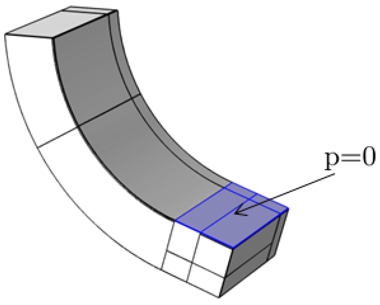
A zero pressure inlet condition is put on the inlet at the leading edge and a zero pressure outlet condition on the outlets of the fluid domain. In the LEG, a velocity condition normal to the inlet hole is used, the value of this velocity is such that the supply flow Q s is satisfied given the area of the inlet, which is determined by its radius r i . Moreover, the pressure in the domain of the LEG portion adjacent to the imaginary shaft was constrained to zero. This is further illustrated in Figure 5. A non-slip sliding wall condition was put on the fluid–shaft interface and on the fluid-bearing interface a stationary wall condition was used. The turbulence variables k and ω were prescribed at the inlets by specifying a turbulent length scale and intensity at the default values that COMSOL suggests. As a test, simulations were performed using both zero and a high turbulence intensity with a negligible difference results wise.

3.4.2. Thermal

Constant temperatures T i 2 and T i were prescribed at the fluid domain leading edge inlet and at the LEG injection hole, respectively. Outflow conditions were put on the outlets and a convection condition was used on the pad external surfaces at temperature T c and convection coefficient h c . As for the fluid–shaft interface, the locally insulated condition from [25] was used, stating that T ¯ · n = 0 at each point along the fluid–shaft interface boundary, where n is its outward normal. For the inlet temperature in Pad A, the simple mixing formula from [6] was used.

3.4.3. Mesh Deformation

As mentioned earlier, the fluid–shaft surface was prescribed a normal displacement of d 0 + h ( θ ) . The fluid domain outlets and leading edge inlet were constrained to deform with a zero normal displacement.

4. Simulation

The numerical values for the bearing characteristic parameters are summarized in Table 1.
Moreover, the parameters for the lubricant are those typically associated with the standard ISO VG 32. Explicit values are given by A = 0.0000736317, B = 797.7122 , C = 177.3562 . These values were also used in e.g., [26].

Finite Element Mesh

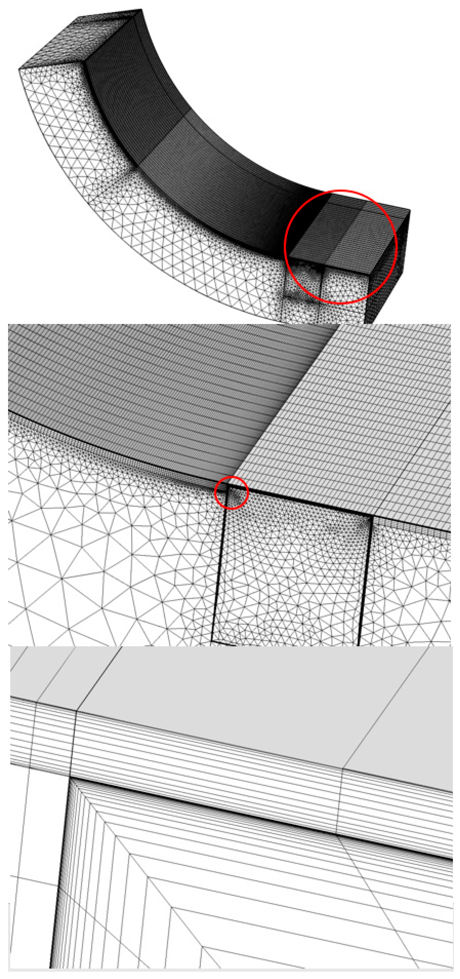
The mesh consists of brick elements in the fluid domain with the exception of the LEG where tetrahedal elements were used along with brick elements clustered to the wall, as illustrated in Figure 6.
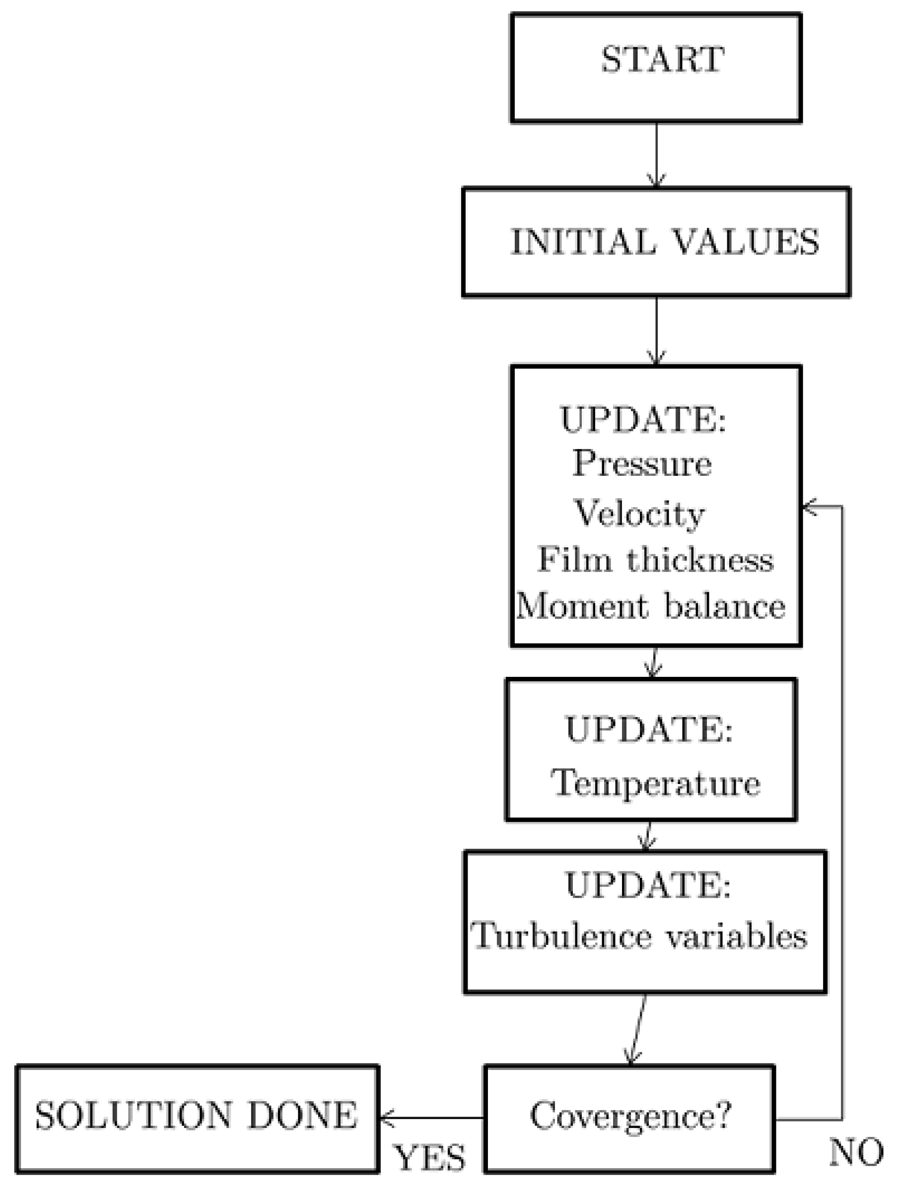
The babbit coating was meshed with brick elements and the remaining, bulk part, of the pad was meshed with tetrahedal elements. Only linear shape functions were used. Since the turbulence variables k and ω proved very sensitive to the wall resolution in the groove, a total of 20 layers were used with an initial thickness of 1 μ m and a stretching factor of 1.3 . Using this mesh, the maximum y + values was always such that y + < 11 , which is typically considered as a well resolved boundary layer. More specifically, the mesh on the bulk part of the pad was made up by 101,509 tetrahedals and 3255 pyramids; the babbit coating mesh consisted of 6510 hexahedral elements; the mesh in the LEG consisted of 34,973 tetrahedals, 1107 pyramids, 38,352 prisms and 13,100 hexahedrals; finally, the deforming part of the fluid domian consisted of 45,360 hexahedrals with 12 elements, most of them close to the walls as illustrated in Figure 6, across the film thickness, 160 elements along the circumferential direction with a higher density closer to the inlet and, finally, 18 elements across (half) the axial length. To assess the grid independence of the simulations, this mesh was refined by using twice the amount of elements in the axial and circumferential direction and 16 elements across the film thickness. The mesh in the LEG was also refined, by cutting the maximum element size in half. This refinement was only done for the fluid domain with the exception of the upper LEG domain, adjacent to the journal, where the number of elements in the circumferential direction could not be increased without causing the meshing algorithm to crash. It was, however, deemed that this part of the mesh was already fine enough. With this refined mesh, the relative differences between maximum temperature- and pressure were 0.4 % and 3.5 % , respectively, or, in absolute terms, 1.5 K and 0.24 MPa. Due to the rapid increase in computational burden with the finer mesh, the original mesh was deemed as an acceptable trade-off between accuracy and numerical efficiency. Moreover, the relative tolerance level was put to 0.01. The reason for this relatively high value was that the convergence rate was very slow while still the solution monitoring probes exhibited a more or less steady state behavior well before a relative solution error of 0.01 was passed. This indicates that it is probable that the solution was converged in an averaged sense. Moreover, a schematic scheme of the iteration process is outlined in Figure 7. In each update block, the variables are solved for simultaneously using a damped Newton algorithm.

5. Results and Discussion

In Section 5.1, the results from the simulations on the original geometry of Pad B are compared, in terms of surface coating temperature, pressure, film thickness and turbulent through molecular viscosity ratio in the mid (symmetry) plane, with those from Pad A. In Section 5.2 and Section 5.3, in order to study the influence of the LEG geometry, the same type of results are presented for Pad B as the size of the LEG portion is stepwise reduced to a more realistic one. Finally, in Section 5.4, the rotational speed of the journal is increased to see if the potential flow disturbances, here quantified by turbulent through molecular viscosity ratio, caused by the LEG becomes increasingly pronounced as the speed increases. The reason for starting with a somewhat over sized LEG portion is because it allowed for a much better convergence of the Newton algorithm that COMSOL uses. Also note that the circumferential coordinate in the following plots start from the leading edge of Pad A.

5.1. Pad A vs. Pad B

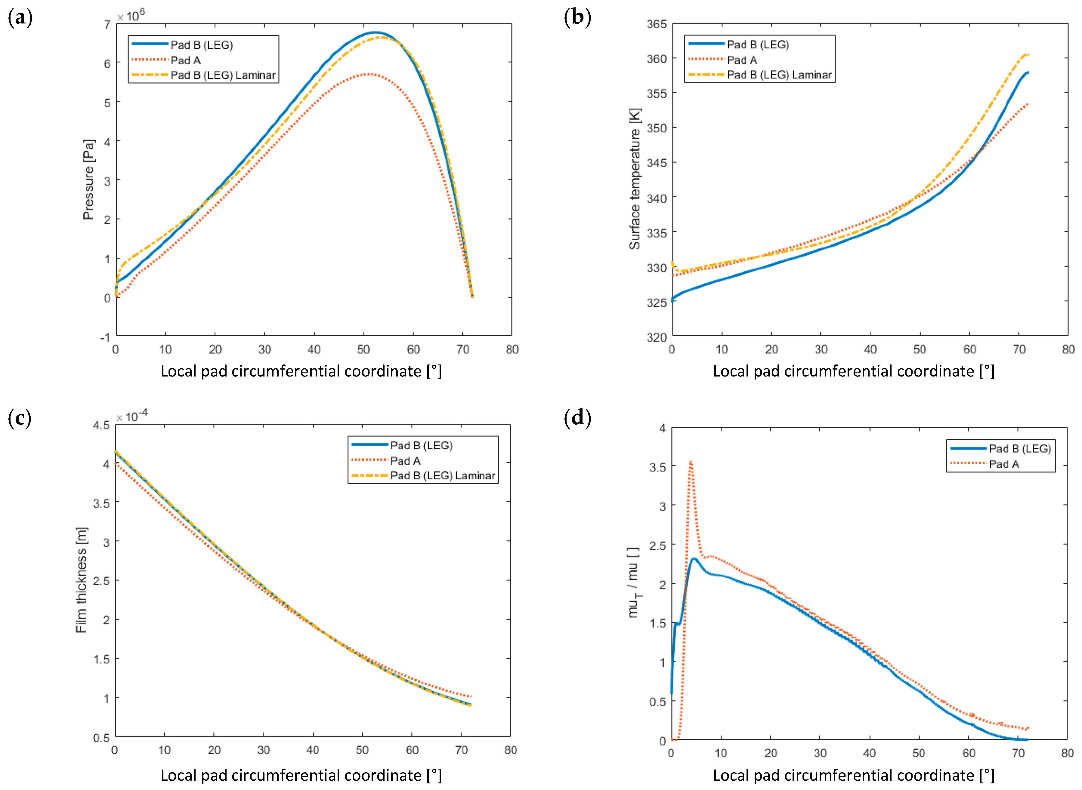
As can be seen from Figure 8a, excluding the LEG geometry from the model (Pad A) estimates a lower load carrying capacity and a somewhat lower maximum pressure. It is also noted than the Pad B models (LEG) manage to capture some of the ram pressure feature that is commonly observed at the inlet of tilting pad bearings; this is even more notable for the laminar model than the turbulent. From Figure 8b, it is observed that the Pad A model (no LEG) yields approximately a 5 ° C higher inlet temperature. It does, however, predict a lower maximum mid plane pad surface temperature than the Pad B model (LEG) due to the lower slope of the curve towards the trailing edge of the pad. The higher temperature slope towards the trailing edge, predicted by the Pad B model (LEG), is typically associated with a transition from turbulent to laminar flow with an accompanying lower heat conduction within the lubricant. This phenomena has also been discussed in e.g., [17]. Now, although the maximum pad surface temperature decreases with increased turbulence, relative to the laminar case, it should be clear that the average temperature in the lubricant increases with increased turbulence due to the increased amount of viscous dissipation. With the above discussion in mind, it would thus be expected that the degree of turbulence, here measured as the ratio between eddy(turbulent) viscosity and molecular viscosity, would be higher in the case of Pad A (no LEG) compared to Pad B (LEG). Although small, it is evident from Figure 8d that such is the case. Moreover, the laminar model predicts a higher inlet temperature and a slightly higher maximum temperature than the turbulent one. The film thicknesses are pretty much equal between the models; however, the Pad B model (LEG) does predict a lower minimum thickness than the Pad A model (no LEG), as is seen from Figure 8c.

5.2. Modified Pad B—Shrinking the Length of the LEG Portion

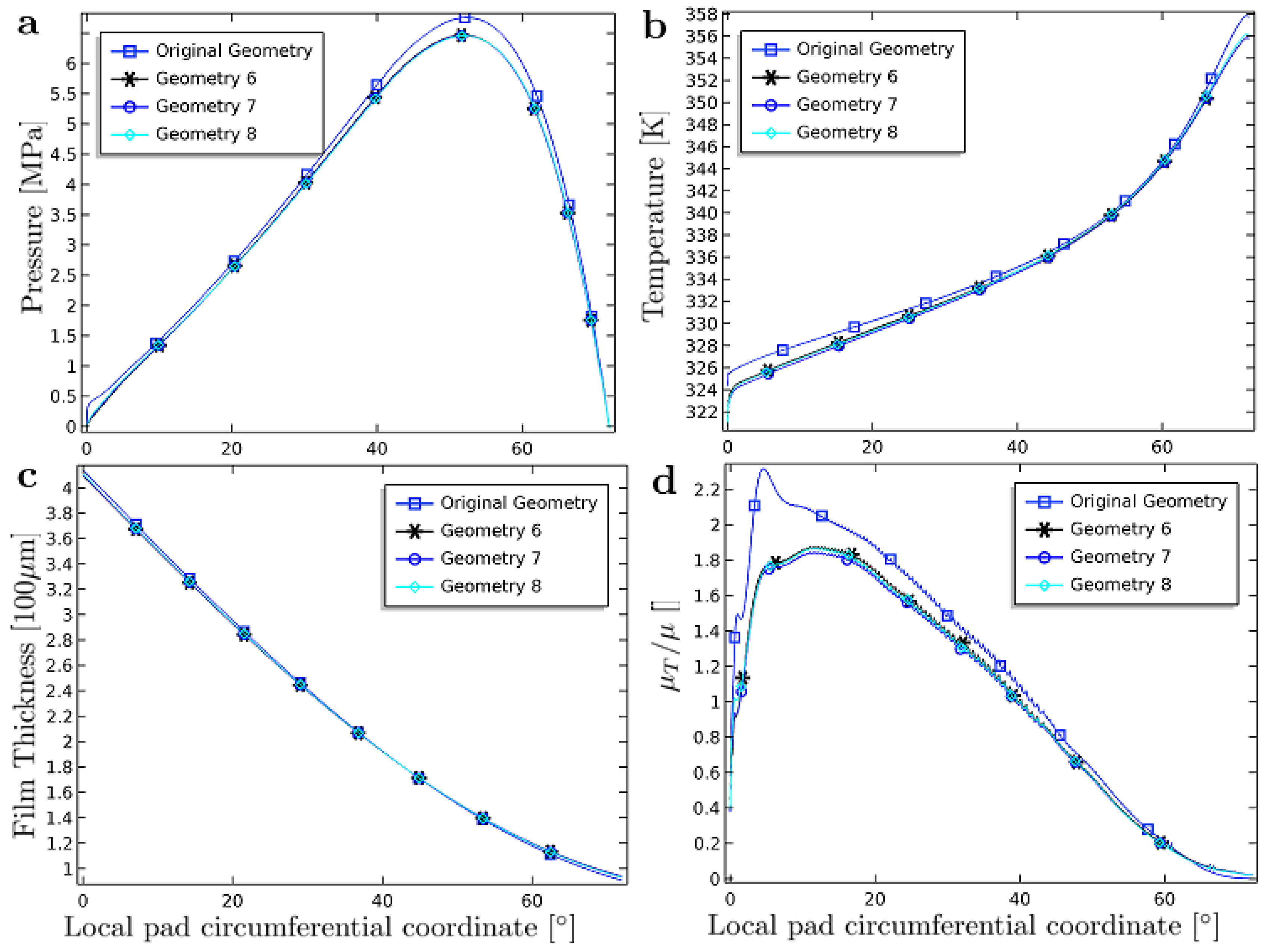
The parameters for the new geometry cases are given in Table 2. Moreover, the different cases considered are numbered in ascending order where Case 1 corresponds to the original geometry. Furthermore, the groove depth L 3 and the inlet radius r i were here kept constant at X m (see Table 1 for input data). The different cases are denoted as “Geometry 2–6” in Figure 9.
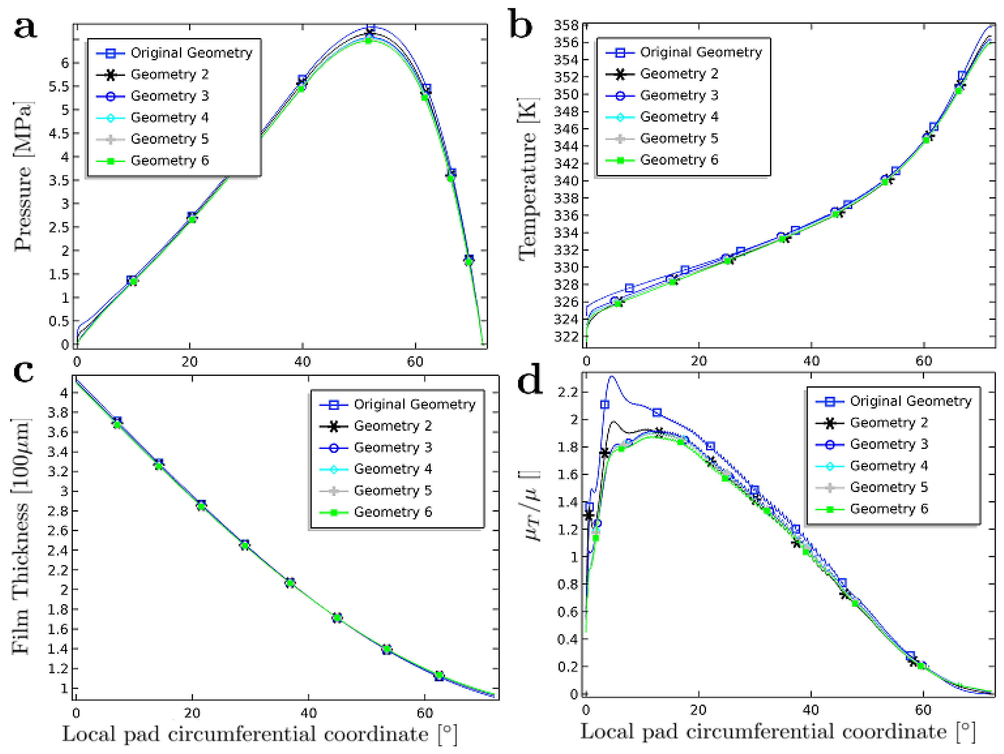
As seen in Figure 9a, the mid plane pressure profiles show a very similar behavior across the different cases. One notable difference is that of the inlet pressures where the effect of the ram pressure diminishes as the LEG portion gets smaller; this also has the effect of reducing the maximum pressure. From Figure 9b, a somewhat lower inlet temperature and a lower gradient, accompanied by a lower maximum temperature, towards the trailing edge are obtained as the LEG portion shrinks. The latter agrees with the results in Figure 9d where the level of turbulence towards the trailing edge gets higher as the dimensions of the LEG decreases. Moreover, as seen in Figure 9c, the film thicknesses across the geometry sweep all but coincides. From Figure 9 as a whole, it is evident that changing the parameters determining the length of the LEG geometry to some more realistic values does not have a significant impact on the simulation results in terms of pressure, temperature, film thickness and level of turbulence.

5.3. Modified Pad B—Shrinking the Depth of the LEG

Two different depths, controlled by the parameter L 3 , are investigated, see Table 3, while L 1 and L 2 are kept constant at L 1 = 0.025 m and L 2 = 0.015 m, which corresponds to Case 5 from Section 5.2. These two new cases are denoted Case 7 and 8; moreover, they are denoted in Figure 10 as “Geometry 7” and “Geometry 8”, respectively.
From Figure 10a, it is observed that the mid plane pressure profile remains almost the same as the groove depth is diminished. The same observation is made concerning the mid plane surface temperature profile in Figure 10b, the film thickness profile in Figure 10c and the turbulent to molecular viscosity ratio in Figure 10d. However, a somewhat peculiar result is spotted in Figure 10d where the level of turbulence first reduces, relative to Geometry 6, when the groove depth is set to L 3 = 0.0308 only to increase again when the depth is further reduced to L 3 = 0.0154 ; the difference is, however, as previously mentioned, very small.

5.4. Modified Pad B vs. Pad A—Increasing the Rotational Speed

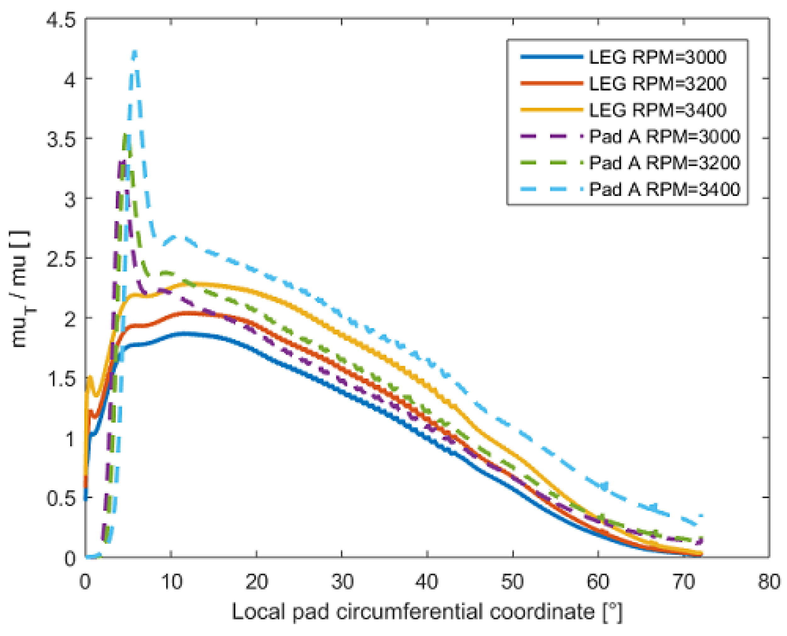
Finally, the rotational speed of the journal was varied between 3000–3400 rpm in order to study its influence on the turbulence levels. The geometry used was the one defined by L 1 = 0.025 , L 2 = 0.015 , L 3 = 0.0462 , which corresponds to Case 5 (Geometry 6).
From Figure 11, observing the ratio of turbulent to molecular viscosity as a function of rotational speed, it seems as the Pad A model inherently generates more turbulence compared to the Pad B (LEG) model. This is in direct contrast to the notion of He et al. [7] that the LEG portion causes an increase of turbulence.

5.5. Turbulence Levels as a Function of Axial Position

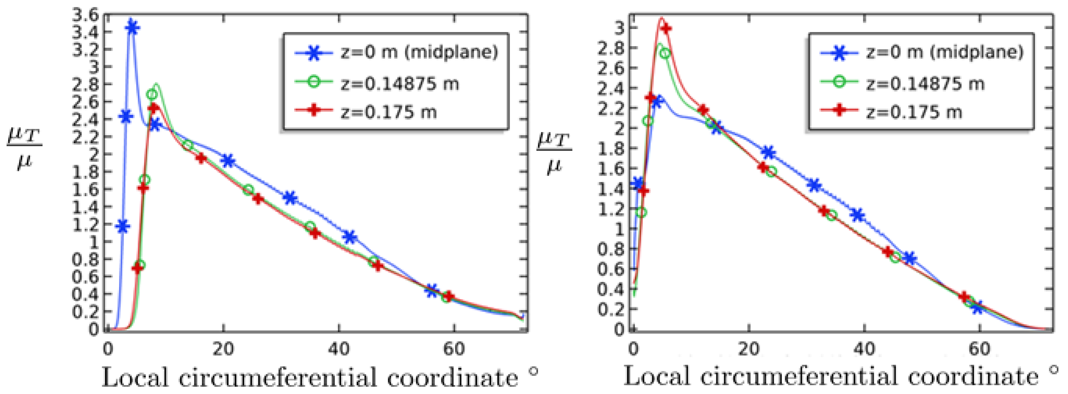
So far, only the turbulence levels in the mid plane(symmetry plane) have been studied. As it turns out, when the same ratio, i.e., μ T μ , is plotted at axial positions z = 0.14875 m and z = 0.175 m (i.e., at the axial end), an interesting feature, which is illustrated in Figure 12, reveals itself. The geometry used for the LEG in Pad B corresponds to its original geometry.
As can be seen from Figure 12, the turbulence levels in Pad B (LEG) show a decreasing trend when plotted further away in the axial direction from the mid plane while the opposite is true for Pad A. Moreover, when the volume average of the ratio μ T / μ is calculated in the two pads, Pad B (LEG) actually has a slightly higher value than Pad A, although they only differ by about 4.5 % . More specifically, the calculated volume average values of the ratio μ T / μ are 0.66 and 0.63 for Pad B (LEG) and Pad A, respectively. When, instead of the original geometry, the more realistic geometry Geometry 6 is used; then, Pad A has the highest volume averaged value of μ T / μ . The differences are, however, very small, differing by ∼3%. This supports the notion indicated by He et al. [7] but is certainly not convincing. However, the maximum value of μ T / μ in both of the pads is found in Pad A for each case and it is located in the mid plane. These maximum levels are 3.6 versus 3.1 for Pad A and Pad B (LEG), respectively, hence differing by roughly 14%. The reason for the increasing levels of turbulence towards the axial ends in Pad B (LEG) is believed to be due to the presence of the corner in the LEG, which presents a severe geometrical disturbance to the flow.
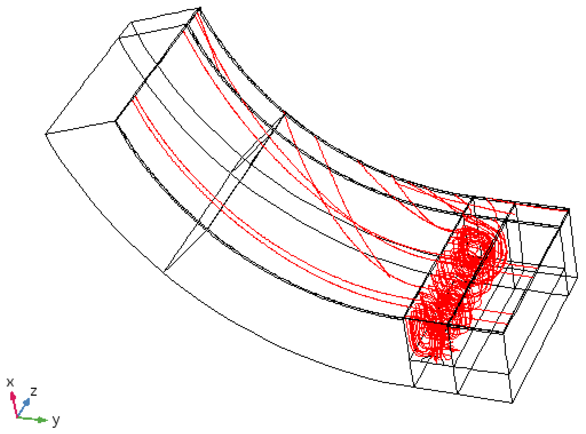
The reason as to why the LEG geometry seems to have a dampening effect on the mid plane turbulence in this model compared to the case of the no LEG model is a bit unclear to the authors; one explanation however may be given by considering the lubricant stream lines in the LEG. From Figure 13, it seems as the lubricant settles into what looks like a swirling, vortex like, flow in the LEG. This type of swirling flow pattern, although in 2D, was also obtained by DeCamillo et al. [8] in their CFD analysis of the LEG. Now, this “ordering” of the flow may be the reason as to why the turbulence, or loosely speaking, “randomness” is predicted to decrease in the mid plane when an LEG is present compared to the case where it is not. Another interesting feature is the presence of the inlet ram pressure in the LEG pad which is not present in the case of no LEG pad even though it does exist in these cases, as shown experimentally by, e.g., [27]. It is possible that including this phenomena would have a notable effect on the downstream flow characteristics. Lastly, it should also be mentioned that the simulation results obtained here are only as good as the turbulence model used, which, although sophisticated compared to standard lubrication theory, is subject to a number of simplifications, which makes it hard to evaluate the validity of the results quantitatively, or even qualitatively, without comparing with experimental data. As such, the investigation carried out in this paper should be taken more as an attempt to shed some light on the highly complex business of turbulence in tilting pad journal bearings in the presence of an LEG and it is recognized that the need for corresponding experimental data is a necessity. Hence, the authors make no claims that the results presented in the present study are valid in the general case. However, the results from the two models (which are designed to model the same bearing) still show a rather big difference in terms of temperature and pressure; this in itself is believed to be an important result for the continued modeling of more and more realistic fluid film bearing geometries.

6. Conclusions

The simulations show that, in essence:
  • The effective temperature boundary condition in Pad A seems to overestimate the inlet temperature compared to Pad B. The difference is quite small however.
  • The LEG pad is predicted to have a lower level of turbulence than the conventional pad in the mid plane, the difference becomes even larger as the speed increases. It is however predicted to have a slightly higher value of turbulence when looking at the volume average compared to Pad A. Moreover, the maximum value of turbulence levels is found in the mid plane of Pad A. This makes it so that any conclusion regarding the hypothesis put out by He et al. [7] cannot be stated without a serious amount of skepticism and so this research question cannot be resolved based on the findings of the present study.
  • The LEG pad yields a higher maximum pad surface temperature due to the typical transition from turbulent to a laminar flow towards the trailing edge being more prominent than in the no LEG case. This result is further supported by considering Figure 8d which shows that the level of turbulence is indeed somewhat lower for the LEG pad towards the trailing edge.
  • The dimensions of the LEG portion has a surprisingly modest influence on the downstream flow characteristics.
  • In future similar investigations, the ram pressure should be accounted for in the model for the conventional (no LEG) pad since this might have an notable impact on the down stream flow characteristics.
  • As with any attempt to simulate turbulent flow, the findings of the present study must be used with great caution until more refined studies and/or experimental data are available for comparison.

Author Contributions

Formal Analysis, P.C.; Supervision, A.A. and R.L.; Writing—Original Draft, P.C.; Writing—Review and Editing, A.A. and R.L.

Funding

The work has been supported by the European project FLEXTURBINE in the H2020 research and innovation programme under Grant No. 653941 and by using the resources of High Performance Computing Center North (HPC2N). The financial support from FLEXTURBINE is highly appreciated by the authors.

Conflicts of Interest

The authors declare no conflict of interest.

References

  1. Mikula, A.M.; Gregory, R.S. A comparison of tilting pad thrust bearing lubricant supply methods. J. Lubr. Technol. 1983, 105, 39–45. [Google Scholar] [CrossRef]
  2. Mikula, A.M. Further test results of the leading-edge-groove (leg) tilting pad thrust bearing. ASME J. Tribol. 1988, 110, 174–180. [Google Scholar] [CrossRef]
  3. Bang, K.-B.; Kim, J.-H.; Cho, Y.-J. Comparison of power loss and pad temperature for leading edge groove tilting pad journal bearings and conventional tilting pad journal bearings. Tribol. Int. 2010, 43, 1287–1293. [Google Scholar] [CrossRef]
  4. Harangozo, A.V.; Stolarski, T.A.; Gozdawa, R.J. The effect of different lubrication methods on the performance of a tilting-pad journal bearing. Tribol. Trans. 1991, 34, 529–536. [Google Scholar] [CrossRef]
  5. Brockwell, K.W.S.A.; Dmochowski, W.; DeCamillo, S.; Mikula, A. Performance evaluation of the leg tilting pad journal bearing. In IMechE Seminar Plain Bearings: Plain Bearings: Energy Efficiency and Design; IMechE: London, UK, 1992; pp. 51–58. [Google Scholar]
  6. Dmochowski, W.K.S.A.; Brockwell, K.; DeCamillo, S.; Mikula, A. A study of the thermal characteristics of the leading edge groove and conventional tilting pad journal bearings. J. Tribol. 1993, 115, 219–226. [Google Scholar] [CrossRef]
  7. He, M.; Allaire, P.E.; Barrett, L.; Nicholas, J. Tehd modeling of leading edge groove tilting pad bearings. In Proceedings of the 6th International Conference on Rotor Dynamics (IFTOMM), Sydney, Australia, 30 September–4 October 2002. [Google Scholar]
  8. Edney, S.L.; Heitland, G.B.; DeCamillo, S.M. Testing, analysis, and cfd modeling of a profiled leading edge groove tilting pad journal bearing. In Proceedings of the ASME 1998 International Gas Turbine and Aeroengine Congress and Exhibition, Stockholm, Sweden, 2–5 June 1998; pp. 2–5. [Google Scholar]
  9. Varela, A.C.; García, A.B.; Santos, I.F. Modelling of leg tilting pad journal bearings with active lubrication. Tribol. Int. 2017, 107, 250–263. [Google Scholar] [CrossRef]
  10. Constantinescu, V.N. Analysis of bearings operating in turbulent regime. J. Basic Eng. 1962, 84, 139–151. [Google Scholar] [CrossRef]
  11. Ng, C.W. Fluid dynamic foundation of turbulent lubrication theory. ASLE Trans. 1964, 7, 311–321. [Google Scholar] [CrossRef]
  12. Ng, C.W.; Pan, C.H.T. A linearized turbulent lubrication theory. J. Basic Eng. 1965, 87, 675–682. [Google Scholar] [CrossRef]
  13. Bouard, L.; Fillon, M.; Frene, J. Comparison between three turbulent models: Application to thermohydrodynamic performances of tilting-pad journal bearings. Tribol. Int. 1996, 29, 11–18. [Google Scholar] [CrossRef]
  14. Bukhari, M.; Jaat, M.; Zaman, I.; Khalid, A. Cfd analysis of thin film lubricated journal bearing. Procedia Eng. 2013, 68, 56–62. [Google Scholar]
  15. Nadia, B.; Mehala, K.; Abdelkader, Y. Numerical analyses of turbulent flow behavior in plain journal bearing. Ind. Lubr. Tribol. 2016, 68, 76–85. [Google Scholar]
  16. Armentrout, R.W.; He, M.; Haykin, T.; Reed, A.E. Analysis of turbulence and convective inertia in a water-lubricated tilting-pad journal bearing using conventional and cfd approaches. Tribol. Trans. 2016, 60, 1129–1147. [Google Scholar] [CrossRef]
  17. Hopf, G.; Schuler, D. Investigations on large turbine bearings working under transitional conditions between laminar and turbulent flow. ASME J. Tribol. 1989, 101, 628–634. [Google Scholar] [CrossRef]
  18. Gardner, W.W.; Ulschmid, J.G. Turbulence effects in two journal bearing applications. J. Lubr. Technol. 1974, 96, 15–20. [Google Scholar] [CrossRef]
  19. Monmousseau, P.; Fillon, M. Transient thermoelastohydrodynamic analysis for safe operating conditions of a tilting-pad journal bearing during start-up. Tribol. Int. 2000, 33, 225–231. [Google Scholar] [CrossRef]
  20. Menter, F.R.; Kuntz, M.; Langtry, R. Ten years of industrial experience with the sst turbulence model. Turbul. Heat Mass Transf. 2003, 4, 625–632. [Google Scholar]
  21. The Menter Shear Stress Transport Turbulence Model. Available online: http://turbmodels.larc.nasa.gov/sst.html (accessed on 5 December 2017).
  22. COMSOL 5.3, cfd User’s Guide; COMSOL Inc.: Stockholm, Sweden, 2017.
  23. Kays, W.M. Turbulent prandtl number: Where are we? J. Heat Transf. 1994, 116, 284–295. [Google Scholar] [CrossRef]
  24. Comsol Multiphysics Reference Manual, Version 5.3; COMSOL Inc.: Stockholm, Sweden, 2017.
  25. Suganami, T.; Szeri, A.Z. A thermohydrodynamic analysis of journal bearings. J. Lubr. Technol. 1979, 101, 21–27. [Google Scholar] [CrossRef]
  26. Knežević, D.; Savić, V. Mathematical Modeling of Changing of Dynamic Viscosity, as a Function of Temperature and Pressure, of Mineral Oils for Hydraulic Systems; Facta Universitatis Series Mechanical Engineering; University of Niš: Beograd, Serbia, 2006. [Google Scholar]
  27. Taniguchi, S.; Makino, T.; Takeshita, K.; Ichimura, T. A thermohydrodynamic analysis of large tilting-pad journal bearing in laminar and turbulent flow regimes with mixing. J. Tribol. 1990, 112, 542–548. [Google Scholar] [CrossRef]
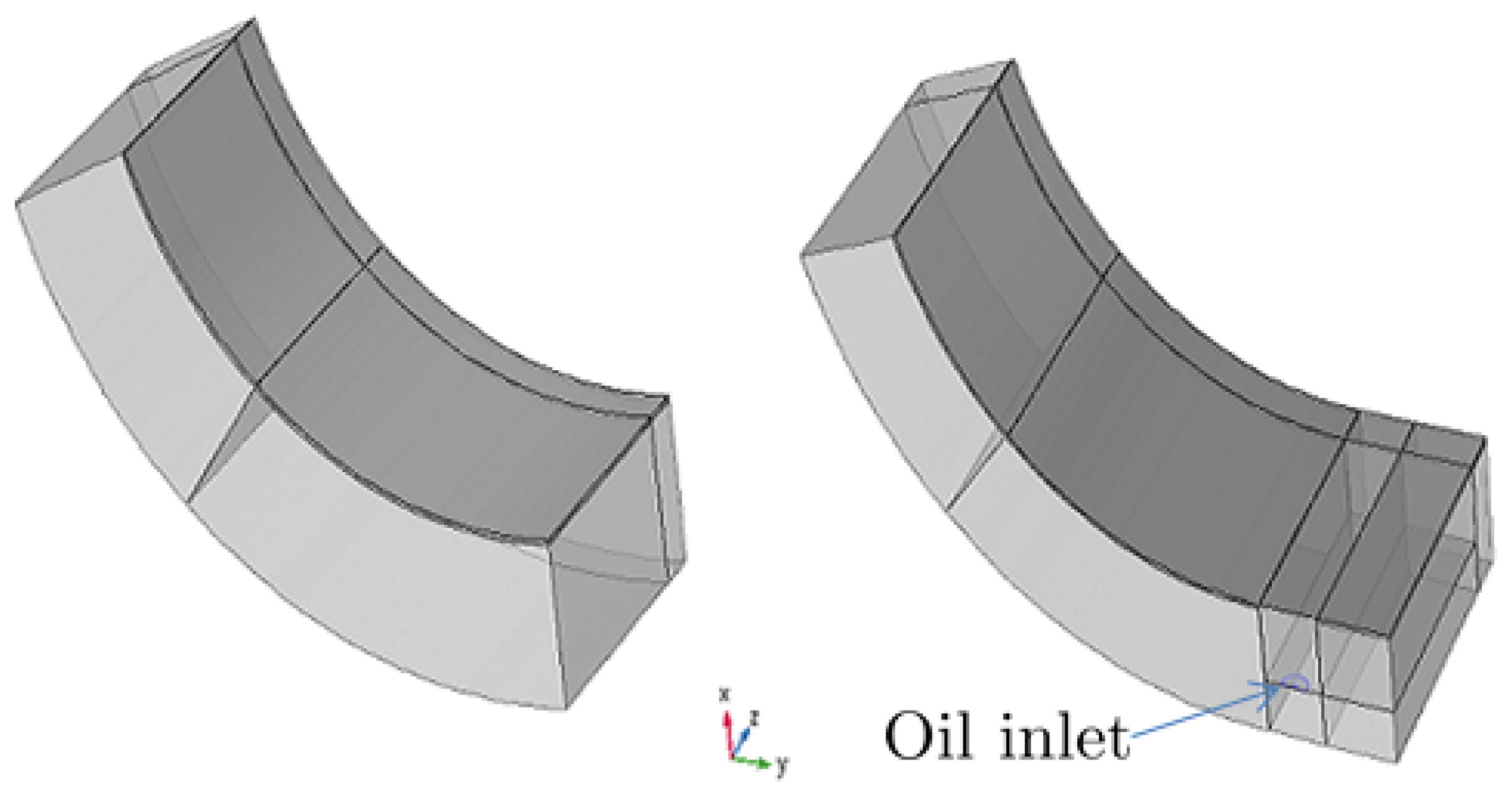
Figure 1. 3D view of Pad A (left) and Pad B (right). Note the inlet hole in the LEG of Pad B, marked with blue color.
Lubricants 06 00097 g001
Figure 2. 3D view of Pad A (left) and Pad B (right). where the fluid- and solid domain of each pad has been marked with blue and gray color, respectively.
Lubricants 06 00097 g002
Figure 3. Close up on the LEG portion of Pad B with the characteristic dimensions L 1 , L 2 , L 3 . Note that only half of the axial length is modeled due to symmetry.
Lubricants 06 00097 g003
Figure 4. View of Pad B in the x y -plane.
Lubricants 06 00097 g004
Figure 5. Further illustration of the zero pressure constraint that was put on the fluid film at the top of the LEG portion.
Lubricants 06 00097 g005
Figure 6. Finite element mesh of Pad B and a close up on the boundary layer and tetrahedal mesh in the LEG, highlighted by the red circle in the upper of the two images.
Lubricants 06 00097 g006
Figure 7. Structure of the numerical iteration scheme that was used in the present study.
Lubricants 06 00097 g007
Figure 8. Comparison of results between Pad A and B, including laminar results: (a) pressure; (b) surface temperature; (c) film thickness; (d) ratio of turbulent through molecular viscosity. All plots are versus the local pad circumferential coordinate at the symmetry plane.
Lubricants 06 00097 g008
Figure 9. Comparison of results between the different geometry cases (Cases 1–6) where the lengths of the LEG geometry ( L 1 and L 2 ) are stepwise diminished: (a) mid plane pressure; (b) mid plane surface temperature; (c) film thickness; (d) ratio of turbulent through molecular viscosity. All plots are versus the local pad circumferential coordinate.
Lubricants 06 00097 g009
Figure 10. Comparison of results with a varying groove depth ( L 3 ) for constant L 1 and L 2 : (a) mid plane pressure; (b) mid plane surface temperature; (c) film thickness; (d) ratio of turbulent through molecular viscosity. All plots are versus the local pad circumferential coordinate.
Lubricants 06 00097 g010
Figure 11. Comparison of turbulent to molecular viscosity ratio between Pad A and Pad B for different values of rotational speed. The geometry corresponds to Geometry 6.
Lubricants 06 00097 g011
Figure 12. Comparison of turbulent to molecular viscosity ratio between Pad A (left) and Pad B (right) (LEG) for different values of the axial coordinate z corresponding to z = 0 m, z = 0.14875 m, z = 0.175 m. The geometry used in Pad B corresponds to its original geometry.
Lubricants 06 00097 g012
Figure 13. Flow patterns in the original geometry (Case 1). The lubricant flows from right to left and mixes in the LEG before traveling along the pad towards the trailing edge. Note that this is only half of the pad in the axial coordinate (axial symmetry).
Lubricants 06 00097 g013
Table 1. Bearing characteristic parameters.
ParameterValueDescription
R b 0.25 [m]Bearing radius
L0.350 [m]Bearing axial length
t p 0.075 [m]Pad thickness
t b 0.002 [m]Babbit thickness
m0.25 []Pad preload
k r 1.28‰Relative clearance
β 72 ° Pad arc length
p0.6 []Pivot offset
e x 0 [m]Journal x-eccentricity
e y −2 × 10 4 [m]Journal y-eccentricity
N3000 s 1 Journal revolutions per minute
T i 320 [K]Lubricant injection temperature
T i 2 320 [K]Lubricant leading edge inlet temperature
T c 323.15 [K]Convection temperature for the external pad surfaces
h c 400 [ W m 2 K ] Convection coefficient for the pad external surfaces
Ψ 225 ° Pivot position in the circumferential coordinate θ
Q s 0.00175 [ m 3 s ]LEG supply flow
L 1 0.04 [m]Original length of the LEG
L 2 0.05 [m]Original length of the pad portion preceding the LEG
L 3 0.0462 [m]Original depth of the LEG = 0.6 ( t p + t b )
r i L 1 4 [m]Radius of the circular inlet hole in the LEG
Table 2. Bearing characteristic parameters for the shrunken LEG portion.
Case23456
L 1 [m]0.030.0250.0250.0250.025
L 2 [m]0.040.0350.0250.020.015
Table 3. Different values for the paramter L 3 which sets the depth of the LEG.
Case78
L 3 [m]0.03080.0154