Dynamic Analysis of Radial Journal Bearing-Rotor System Based on the Meshless Barycentric Rational Interpolation Collocation Method

Abstract

This study focuses on a rigid rotor supported by radial journal bearings. Initially, models for the unsteady oil film force in bearing lubrication and the dynamics of the bearing-rotor system are established. Subsequently, the Reynolds equation for dynamic lubricating oil films is discretely solved using the meshless barycentric rational interpolation collocation method. By combining this with the equation of motion for the axis orbit, the oil film pressure distribution, the dynamic response of the rotor, and the axis orbit are calculated. Furthermore, the study investigates the dynamic response of the rotor at different rotational speeds, both with and without considering unbalanced loads. Finally, the influence of step load on the stability of rotor motion is analyzed, revealing that applying an appropriate step load to the rotor can effectively mitigate the lubricating oil films oscillation conditions. The findings of this study hold significant reference value and practical utility for engineering applications.

1. Introduction

Rotating machinery plays a pivotal role in engineering fields such as aerospace and power generation, with its operational efficiency and reliability largely determined by the performance of the sliding bearing-rotor system. In recent years, with the rapid development of rotating machinery, more and more people have gradually recognized the importance of stable operation of the bearing-rotor system. Many scholars have analyzed and discussed the dynamic behavior of bearing-rotor systems using various methods. Currently, analytical solutions for dynamic differential equations of multi-degree-of-freedom nonlinear vibration systems are not feasible, and numerical solutions are the only option. Traditional methods for solving the transient response of rotor systems mainly include the central difference method, Runge–Kutta method, Newmark–β method, and Wilson–θ method. M. Phani Kumar [1] employed a linearized perturbation method to solve the dynamic coefficients of eccentric bearings and conducted a nonlinear transient analysis of the journal center trajectory to determine the stability of the system. Li [2] used Coleman transformations and complex transformations to obtain a reduced-order system and studied the nonlinear vibration and stability of the system, focusing on the nonlinear vibration and dynamic stability analysis of a nonlinearly supported rotor-blade system. Xiong [3] proposed a dynamic misalignment model that couples rotor dynamics with transient mixed elastohydrodynamic lubrication, and analyzed the impact of misalignment on the performance of bearings under dynamic load slip.

In the field of nonlinear dynamics analysis, considerable work has been carried out by predecessors, and numerous noteworthy achievements have been made. These efforts have allowed us to describe various complex dynamic phenomena in engineering and physics more accurately and deeply, providing a more comprehensive reflection of the dynamic characteristics of actual systems. However, there are still challenges in mastering the dynamic characteristics of multi-degree-of-freedom nonlinear systems, especially when it comes to the accurate handling of nonlinear oil film forces in sliding bearings, which directly affects the accuracy of the system’s nonlinear characteristics. Many scholars have diligently sought precise expressions for nonlinear oil film forces. There are two approaches to modeling fluid dynamics problems. On one hand, there are models based on the Navier–Stokes equations. Wang [4] employed an oil film force model with eight linearized stiffness and damping coefficients to evaluate the dynamic response of the nonlinear dynamics of the oil film bearing-rotor system. Gu [5] explored the static characteristics of water-lubricated sliding bearings under three-dimensional slip velocity boundary conditions using the CFD method. On the other hand, some models are based on the Reynolds equation. B. Sivák and M. Sivák. [6] obtained numerical solutions to the Reynolds equation using the modified Ritz method. J.W. Lund [7] modeled the bearing as two orthogonal spring-dampers with eight linearized stiffness and damping coefficient oil film force models, which was later used by Xie [8] to study the dynamic response of circular pad bearings and rotors. Capone presented an exact analytical solution for the nonlinear oil film forces of radial sliding bearings under the short bearing assumption, which is fast and convenient. Many scholars, such as Weimin [9] and Xiang [10], have based their studies on this model to explore the dynamic laws of bearing-rotor systems. Zhang [11] used the variational principle and the method of separation of variables to obtain the oil film pressure distribution. Jin [12,13] studied the characteristics of tilting-pad radial sliding bearings using a database approach. Numerical methods for solving the Reynolds equation include: Gu [14] used the finite difference method to solve the Reynolds equation and investigate the static characteristics of aerostatic porous journal bearings. Xie [15] et al., based on the modified Reynolds equation, used the finite difference method to investigate the lubrication mechanism and performance parameters considering wall slip and inertial forces. K.V. Avramov [16] utilized the finite element method to obtain the oil film pressure of a long journal bearing and conducted a stability analysis of the rotor. Chris A. Papadopoulos [17] established a rotor-bearing system using the finite element method and proposed a model for identifying the clearance between the rotor and the bearing.

So far, the following methods have been commonly used to obtain nonlinear oil film forces: the oil film force model with eight linearized coefficients cannot explain complex dynamic characteristics; the variational method has relatively low computational accuracy; the finite difference method directly numerically solves the Reynolds lubrication equation, which has high computational accuracy but low efficiency; and the database fitting method offers both good computational accuracy and speed, but requires a pre-existing database. Due to reasons such as heavy computational workload or low accuracy, these methods are difficult to apply to the nonlinear dynamic analysis, research, and design of actual bearing-rotor systems.

The above research mainly focuses on grid-based methods. However, for large-deformation free-surface flows of fluids, the meshless methods have inherent advantages over grid-based methods in solving fluid problems. Therefore, Li [18] and Shi [19] analyzed the air bearing lubrication model in the head-disk drive system using the Least Squares Method and the MLPG meshless method, respectively. They derived the pressure distribution patterns and compared the results with those obtained from finite element and finite difference methods. Jiangang [20] studied radial sliding bearings using Radial Basis Functions. Although they achieved preliminary research results on radial sliding bearings, there is a lack of in-depth research on the dynamic behavior of bearing-rotor systems using the meshless methods.

In this paper, a rigid rotor system supported by a radial journal bearing is taken as the research object. Firstly, a nonlinear oil film force model of the radial sliding bearing is established based on the meshless barycentric rational interpolation theory. Then, the nonlinear dynamic equations coupling the transient lubricating oil film force and the rotor are derived. Finally, the coupled nonlinear dynamic equations are numerically solved. Additionally, a series of parametric studies on the bearing-rotor system are conducted. The variation of vibration response with operating conditions is obtained through the axis orbit and phase diagrams, in order to evaluate the effects of rotational speed and unbalanced load on the axis displacement response, oil film thickness, and oil film force. Especially, applying appropriate step loads can effectively improve the oil film oscillation. The research results provide a solid foundation for the vibration response analysis of such rotating systems.

2. Meshless Barycentric Rational Interpolation Collocation Method

2.1. The One-Dimensional Barycentric Interpolation Formula and Its Differentiation Matrix

For the interval [a, b] discretized as $=x_1<x_2<\cdots <x_n=b$, with the function values at the nodes given by $u_k=u\left(x_k\right),k=\mathrm{1,2},\cdots ,n$, the barycentric interpolation function for the function $u\left(x\right)$ is given by [21,22,23]:

$$u\left(x\right)={\sum }_{k=1}^n{L}_k\left(x\right)u_k$$

(1)

The basis function for the barycentric interpolation is:

$$L_k\left(x\right)={\displaystyle \frac{\frac{{\omega }_k}{x-x_k}}{{\sum }_{j=1}^n\frac{{\omega }_j}{x-x_j}}},k=\mathrm{1,2},\cdots ,n$$

(2)

where the interpolation weights ${\omega }_k$ for the barycentric rational interpolation formula are:

$${\omega }_k={{\sum }_{i\in J_k}\left(-1\right)}^i{\prod }_{j=i,j\ne k}^{i+d}{\displaystyle \frac{1}{x_k-x_j}},k=\mathrm{1,2},\cdots ,n$$

(3)

Then Equation (3) represents the barycentric rational interpolation at the nodes $x_1,x_2,\cdots ,x_n$.

The m-order derivative of the function $u\left(x\right)$ at the nodes can be represented as:

$$u_i^{\left(m\right)}:=={\sum }_{j=1}^n{L}_j^{\left(m\right)}\left(x_i\right)u_j={\sum }_{j=1}^n{D}_{ij}^{\left(m\right)}{u}_j$$

(4)

Written in matrix form as:

$${\mathit{u}}^{\left(m\right)}={\mathit{D}}^{\left(m\right)}\mathit{u}$$

(5)

2.2. The Two-Dimensional Barycentric Interpolation Formula and Its Partial Differentiation Matrix

By discretizing the intervals [a, b] and [c, d] into m and n interpolation nodes respectively, we have $a=x_1<\cdots <x_m=b$ and $c=y_1<\cdots <y_n=d$, resulting in m × n tensor-type interpolation nodes $\left(x_i,y_j\right)$, where $i=\mathrm{1,2},\cdots ,m$ and $j=\mathrm{1,2},\cdots ,n$ [24,25].

The barycentric interpolation format for the function $u(x,y)$ at the nodes $\left\{(x_i,y_j),i=\mathrm{1,2},\cdots ,m;j=\mathrm{1,2},\cdots ,n\right\}$ can be written as:

$$u(x,y)={\sum }_{i=1}^m{\sum }_{j=1}^n{\xi }_i(x){\eta }_j(y)u_{ij}$$

(6)

The ($l+k$)th-order partial derivative of the function $u(x,y)$ can be written as:

$${\displaystyle \frac{{\mathsf{\partial }}^{l+k}u}{\mathsf{\partial }{x}^l\mathsf{\partial }{y}^k}}={\sum }_{i=1}^m{\sum }_{j=1}^n{\xi }_i^{\left(l\right)}(x){\eta }_j^{\left(k\right)}(y)u_{ij}$$

(7)

The correspondence between the partial derivatives of a differential equation and the differentiation matrix is:

$${\displaystyle \frac{{\mathsf{\partial }}^{l+k}u}{\mathsf{\partial }{x}^l\mathsf{\partial }{y}^k}}\Rightarrow {\mathit{C}}^{\left(l\right)}\otimes {\mathit{D}}^{\left(k\right)}, l,k=\mathrm{0,1},2,$$

(8)

Provides that the above formula ${\mathit{C}}^{\left(0\right)}={\mathit{I}}_m,{\mathit{D}}^{\left(0\right)}={\mathit{I}}_n$.

Where: the symbol $\otimes$ denotes the Kronecker product of the matrix. ${\mathit{C}}^{\left(l\right)},{\mathit{D}}^{\left(k\right)}\left(l,k=\mathrm{1,2},\cdots \right)$ are Meshless barycentric rational interpolation collocation method $l$th-order and $k$th-order differential matrices with respect to the nodes $x_1,x_2,\cdots ,x_m$ and $y_1,y_2,\cdots ,y_n$, respectively. ${\mathit{I}}_m$ and ${\mathit{I}}_n$ are the unit matrices of the $l$-order and $k$-order, respectively.

2.3. The Expression of Differential Equations Based on the Differential Matrix

The barycentric interpolation collocation method is a collocation-type numerical method that approximates unknowns based on barycentric interpolation, representing a truly meshless numerical approach. By utilizing the concept of differential matrices, the matrix form calculation formula for the discrete form of the barycentric interpolation collocation method for differential equations can be directly written out.

For ordinary differential equations (ODEs), by replacing the derivative operator with ODEs of the same order, we can obtain the calculation formula for the barycentric interpolation collocation method for ODEs. This applies to ODEs in their general form.

$$a\left(x\right){\displaystyle \frac{d^{2}u\left(x\right)}{d{x}^2}}+b\left(x\right){\displaystyle \frac{du\left(x\right)}{dx}}+c\left(x\right)u\left(x\right)=f\left(x\right)$$

(9)

Substitute Equations (1) and (2) into (9), we find:

$$a\left(x\right){\sum }_{k=1}^n{\displaystyle \frac{d^2{L}_k\left(x\right)}{d{x}^2}}{u}_k+b\left(x\right){\sum }_{k=1}^n{\displaystyle \frac{d{L}_k\left(x\right)}{dx}}{u}_k+c\left(x\right){\sum }_{k=1}^n{L}_k\left(x\right)u_k=f\left(x\right)$$

(10)

Let the equation hold at the computation nodes $x_1,x_2,\cdots ,x_n$, we obtain:

$$\begin{gathered} a\left(x_j\right){\sum }_{k=1}^n{\displaystyle \frac{d^2{L}_k\left(x_j\right)}{d{x}^2}}{u}_k+b\left(x_j\right){\sum }_{k=1}^n{\displaystyle \frac{d{L}_k\left(x_j\right)}{dx}}{u}_k+c\left(x_j\right){\sum }_{k=1}^n{L}_k\left(x_j\right)u_k=f\left(x_j\right), \\ j=\mathrm{1,2},\cdots ,n \end{gathered}$$

(11)

Using the notation of the differential matrix (5), Equation (11) can be written in matrix form as:

$$\left[diag\left(a\left(\mathit{x}\right)\right){\mathit{D}}^{\left(2\right)}+diag\left(b\left(\mathit{x}\right)\right){\mathit{D}}^{\left(1\right)}+diag\left(c\left(\mathit{x}\right)\right){\mathit{I}}_n\right]\mathit{u}=f\left(\mathit{x}\right)$$

(12)

In the formula:

$${a\left(\mathit{x}\right)=\left[a\right(x_1),a(x_2),\cdots ,a(x_n\left)\right]}^T,$$

$${b\left(\mathit{x}\right)=\left[b\right(x_1),b(x_2),\cdots ,b(x_n\left)\right]}^T,$$

$${c\left(\mathit{x}\right)=\left[c\right(x_1),c(x_2),\cdots ,c(x_n\left)\right]}^T,$$

$${f\left(\mathit{x}\right)=\left[f\right(x_1),f(x_2),\cdots ,f(x_n\left)\right]}^T,$$

$$\mathit{u}={u\left(\mathit{x}\right)=\left[u\right(x_1),u(x_2),\cdots ,u(x_n\left)\right]}^T={[u_1,u_2,\cdots ,u_n]}^T.$$

By comparing Equations (9) and (12), one can observe the relationship between the differential equation and its discrete calculation formula using the barycentric interpolation collocation method. The derivatives of the unknown function are replaced by differential matrices of the same order, the coefficients of the unknown function are substituted by diagonal matrices formed by vectors, and the free term function is replaced by its function value vector. Based on this pattern, the calculation formula for the barycentric interpolation collocation method for ordinary differential equations can be conveniently written.

For a general form of second-order partial differential equation.

$$\begin{gathered} a\left(x,y\right){\displaystyle \frac{{\mathsf{\partial }}^{2}u}{\mathsf{\partial }{x}^2}}+b\left(x,y\right){\displaystyle \frac{{\mathsf{\partial }}^{2}u}{\mathsf{\partial }x\mathsf{\partial }y}}+c\left(x,y\right){\displaystyle \frac{{\mathsf{\partial }}^{2}u}{\mathsf{\partial }{y}^2}}+d\left(x,y\right){\displaystyle \frac{\mathsf{\partial }u}{\mathsf{\partial }x}}+e\left(x,y\right){\displaystyle \frac{\mathsf{\partial }u}{\mathsf{\partial }y}}+f\left(x,y\right)u= \\ g\left(x,y\right) \end{gathered}$$

(13)

Similarly, using the notation for differential matrices (8), the calculation formula for the barycentric interpolation collocation method corresponding to Equation (13) can be obtained as follows:

$$\begin{gathered} \left[diag\left(a(\mathit{x},\mathit{y})\right){\mathit{C}}^{\left(2\right)}\otimes {\mathit{I}}_n+diag\left(b(\mathit{x},\mathit{y})\right){\mathit{C}}^{\left(1\right)}\otimes {\mathit{D}}^{\left(1\right)}+diag\left(c(\mathit{x},\mathit{y})\right){\mathit{I}}_m\otimes \\ {\mathit{D}}^{\left(2\right)}+diag\left(d(\mathit{x},\mathit{y})\right){\mathit{C}}^{\left(1\right)}\otimes {\mathit{I}}_n+diag\left(e(\mathit{x},\mathit{y})\right){\mathit{I}}_m\otimes {\mathit{D}}^{\left(1\right)}+ \\ diag\left(f(\mathit{x},\mathit{y})\right){\mathit{I}}_n\right]\mathit{u}=g(\mathit{x},\mathit{y}) \end{gathered}$$

(14)

3. Calculation of Lubrication Equation for Radial Journal Bearings Based on Barycentric Interpolation

3.1. Establishment of a Dynamic Lubrication Model for Radial Journal Bearings

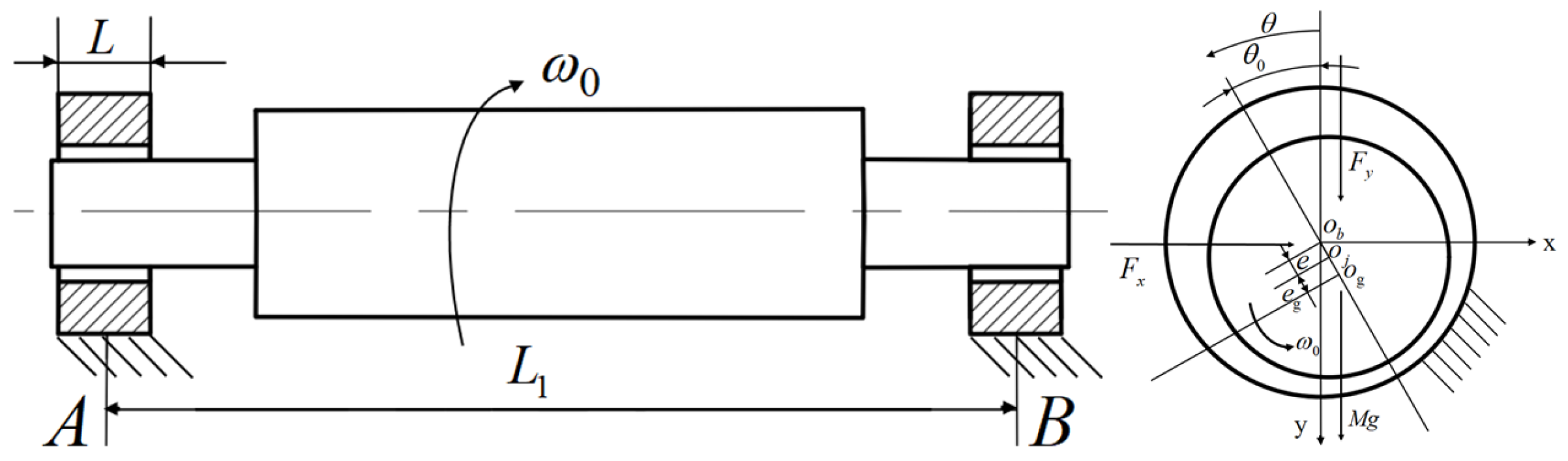
The model of the radial sliding bearing is shown in Figure 1. The geometric center of the rotor is denoted as $O_j$, the centroid of the rotor as $O_g$, and the geometric center of the bearing as $O_b$, with the coordinate origin at $x{O}_{b}y$. The rotor axis describes the dynamic Reynolds equation for the incompressible and laminar flow state of the radial sliding bearing as follows:

$${\displaystyle \frac{1}{R^2}}{\displaystyle \frac{\mathsf{\partial }}{\mathsf{\partial }\theta }}\left({\displaystyle \frac{h^3}{\eta }}{\displaystyle \frac{\mathsf{\partial }p}{\mathsf{\partial }\theta }}\right)+{\displaystyle \frac{\mathsf{\partial }}{\mathsf{\partial }z}}\left({\displaystyle \frac{h^3}{\eta }}{\displaystyle \frac{\mathsf{\partial }p}{\mathsf{\partial }z}}\right)=6{\omega }_0{\displaystyle \frac{\mathsf{\partial }h}{\mathsf{\partial }\theta }}+12{\displaystyle \frac{\mathsf{\partial }h}{\mathsf{\partial }t}}$$

(15)

where R is the bearing radius, $\theta$ is the circumferential calculation coordinate, z is the axial calculation coordinate, h is the oil film thickness, p is the oil film pressure, ${\omega }_0$ is the rotational speed of the rotor shaft, $\eta$ is the viscosity of the lubricating oil, and t is time.

The oil film thickness is defined as follows:

$$h\left(\theta ,t\right)=C+x\left(t\right)\mathit{sin}\theta +y\left(t\right)\mathit{cos}\theta$$

(16)

where C is the bearing radius clearance, $x\left(t\right)$ is the horizontal displacement response, and $y\left(t\right)$ is the vertical displacement response.

Setting $\mathrm{H}=\mathrm{h}/\mathrm{C}$, $Z=\mathrm{z}/\mathrm{L}$, and $\tau ={\omega }_{0}t$, Equation (16) becomes the following dimensionless form

$${\displaystyle \frac{\mathsf{\partial }}{\mathsf{\partial }\theta }}\left(H^3{\displaystyle \frac{\mathsf{\partial }P}{\mathsf{\partial }\theta }}\right)+{\left({\displaystyle \frac{R}{L}}\right)}^2{\displaystyle \frac{\mathsf{\partial }}{\mathsf{\partial }Z}}\left(H^3{\displaystyle \frac{\mathsf{\partial }P}{\mathsf{\partial }Z}}\right)=6{\displaystyle \frac{\mathsf{\partial }H}{\mathsf{\partial }\theta }}+12{\displaystyle \frac{\mathsf{\partial }H}{\mathsf{\partial }\tau }}$$

(17)

where $p=\eta {\omega }_0{\left(R/C\right)}^{2}P$,$H=1+X\mathit{sin}\theta +Y\mathit{cos}\theta$, $X=x/\mathrm{C}$, $Y=\mathrm{y}/\mathrm{C}$.

The dimensionless boundary conditions are: In the axial direction, $P\left(\theta ,-0.5\right)=0$ and $P\left(\theta ,0.5\right)=0$; in the circumferential direction, the initial pressure of the oil film is $P\left(0,Z\right)=0$. the location of oil film rupture is variable, so during the calculation process, any node where $P\left(\theta ,Z\right)<0$ is set to $P\left(\theta ,Z\right)=0$ to determine the end point of the oil film.

Taking the partial derivative of the oil film thickness in Equation (17) with respect to the circumferential direction θ, we obtain:

$${\displaystyle \frac{{\mathsf{\partial }}^{2}P}{\mathsf{\partial }{\theta }^2}}+{\displaystyle \frac{3}{H}}{\displaystyle \frac{\mathsf{\partial }H}{\mathsf{\partial }\theta }}{\displaystyle \frac{\mathsf{\partial }P}{\mathsf{\partial }\theta }}+{\left({\displaystyle \frac{R}{L}}\right)}^2{\displaystyle \frac{{\mathsf{\partial }}^{2}P}{\mathsf{\partial }{Z}^2}}=6{\displaystyle \frac{6}{H^3}}{\displaystyle \frac{\mathsf{\partial }H}{\mathsf{\partial }\theta }}+12{\displaystyle \frac{12}{H^3}}{\displaystyle \frac{\mathsf{\partial }H}{\mathsf{\partial }\tau }}$$

(18)

The Reynolds Equation (18) can be written in a meshless barycentric interpolation discrete format based on the differential matrix Equation (8).

$${[\mathit{C}}^{\left(2\right)}\otimes {\mathit{I}}_n+{\left({\displaystyle \frac{R}{L}}\right)}^2\left({\mathit{I}}_m\otimes {\mathit{D}}^{\left(2\right)}\right)+diag\left[{\displaystyle \frac{3}{\mathit{H}}}{\displaystyle \frac{\mathsf{\partial }\mathit{H}}{\mathsf{\partial }\theta }}\right]\left({\mathit{C}}^{\left(1\right)}\otimes {\mathit{I}}_n\right)]\mathit{P}={\displaystyle \frac{6}{{\mathit{H}}^3}}{\displaystyle \frac{\mathsf{\partial }\mathit{H}}{\mathsf{\partial }\theta }}+{\displaystyle \frac{12}{{\mathit{H}}^3}}{\displaystyle \frac{\mathsf{\partial }\mathit{H}}{\mathsf{\partial }\tau }}$$

(19)

While

$$\mathit{L}={\mathit{C}}^{\left(2\right)}\otimes {\mathit{I}}_n+{\left({\displaystyle \frac{R}{L}}\right)}^2\left({\mathit{I}}_m\otimes {\mathit{D}}^{\left(2\right)}\right)+diag\left[{\displaystyle \frac{3}{\mathit{H}}}{\displaystyle \frac{\mathsf{\partial }\mathit{H}}{\mathsf{\partial }\theta }}\right]\left({\mathit{C}}^{\left(1\right)}\otimes {\mathit{I}}_n\right),\mathit{F}={\displaystyle \frac{6}{{\mathit{H}}^3}}{\displaystyle \frac{\mathsf{\partial }\mathit{H}}{\mathsf{\partial }\theta }}+{\displaystyle \frac{12}{{\mathit{H}}^3}}{\displaystyle \frac{\mathsf{\partial }\mathit{H}}{\mathsf{\partial }\tau }}.$$

Then Equation (19) can be obtained as follows:

$$\mathit{L}\mathit{P}=\mathit{F}$$

(20)

By solving the system of Equation (20), we obtain the numerical solutions for the Reynolds equation, denoted as $P_{\mathrm{2,2}},P_{\mathrm{2,3}},\cdots ,P_{2,\mathrm{n}-1},\cdots ,P_{n-\mathrm{1,2}},P_{n-\mathrm{1,3}},\cdots ,P_{n-1,n-1}$.

The integration of oil film pressure yields the oil film forces in the horizontal and vertical directions.

$$\left\{\begin{array}{c}{F}_x={\int }_0^{2\pi }{\int }_{-0.5}^{0.5}P\mathit{sin}\theta d\theta dZ\\ F_y={\int }_0^{2\pi }{\int }_{-0.5}^{0.5}P\mathit{cos}\theta d\theta dZ\end{array}\right.$$

(21)

3.2. Establishment of a Dynamic Model for a Rigid Rotor-Bearing System

The schematic diagram of the rigid rotor-bearing system is shown in Figure 2. Both the left and right ends of the rotor are supported by symmetrically structured hydrodynamic sliding bearings. The geometric center of the rotor is denoted as $O_j$, the centroid of the rotor as $O_g$, and the geometric center of the bearing as $O_b$, with the coordinate origin at $x{O}_{b}y$. The equation of motion for the rotor axis is as follows:

$$\left\{\begin{array}{c}M\ddot{x}=\eta {\omega }_{0}RL{\left({\displaystyle \frac{R}{C}}\right)}^2{F}_x+M{e}_g{\omega }_0^2\mathit{sin}{\omega }_{0}t+Q_x\\ M\ddot{y}=\eta {\omega }_{0}RL{\left({\displaystyle \frac{R}{C}}\right)}^2{F}_y+M{e}_g{\omega }_0^2\mathit{cos}{\omega }_{0}t+Mg+Q_y\end{array}\right.$$

(22)

where M is the mass of the bearing, $Q_x$ and $Q_y$ are the step loads acting on the rotor, $M\ddot{x}$ and $M\ddot{y}$ are the inertial forces of the rotor borne by the bearing part, $Mg$ is the gravitational force of the rotor acting on the bearing part, and $e_g$ is the mass eccentricity. The Reynolds Equation (18) can be written in a meshless barycentric interpolation discrete format based on the differential matrix Equation (8).

Define the nondimensional variables $\dot{X}=\dot{x}/\left(C{\omega }_0\right)$, $\dot{Y}=\dot{y}/\left(C{\omega }_0\right)$, $\ddot{X}=\ddot{x}/\left(C{\omega }_0^2\right)$, $\ddot{Y}=\ddot{y}/\left(C{\omega }_0^2\right)$, and $\tau ={\omega }_{0}t$. Then, express Equation (22) in a nondimensional form using the state variables $X_1=X$, $X_2=\dot{X}$, $X_3=Y$, and $X_4=\dot{Y}$.

$$\left\{\begin{array}{c}\dot{X_1}=X_2\\ \dot{X_2}={\displaystyle \frac{\eta L}{M{\omega }_0}}{\left({\displaystyle \frac{R}{C}}\right)}^3{F}_x+{\displaystyle \frac{e_g}{C}}\mathit{sin}\tau +q_x\\ \dot{X_3}=X_4\\ \dot{X_4}={\displaystyle \frac{\eta L}{M{\omega }_0}}{\left({\displaystyle \frac{R}{C}}\right)}^3{F}_y+{\displaystyle \frac{e_g}{C}}\mathit{cos}\tau +{\displaystyle \frac{g}{C{\omega }_0^2}}+q_y\end{array}\right.$$

(23)

where $q_x=Q_x/\left(MC{\omega }_0^2\right)$ and $q_y=Q_y/\left(MC{\omega }_0^2\right)$.

4. Analysis of Characteristics of Nonlinear Dynamic Models for Rigid Rotor-Bearing Systems

Set the unbalanced load of the shaft as ${\mathrm{e}}_{\mathrm{g}}$ and the initial values as X = 0, Y = 0, Ẋ = 0, Ẏ = 0. The computational domain is 0 ≤ θ ≤ 2π and −0.5 ≤ Z ≤ 0.5, which is discretized into $m=60,n=60$ equally spaced interpolation nodes, respectively. Then, using the rational interpolation method, the Reynolds equation (17) is discretely solved to obtain the oil film pressure distribution results corresponding to 3600 tensor-type equally spaced interpolation nodes $\left({\theta }_i,Z_j\right)$. The oil film resultant forces $F_x$ and $F_y$ can be obtained from Equation (21). By substituting $F_x$ and $F_y$ into Equation (23) and setting τ = 0, we can calculate ${(\ddot{X}}_0,{\ddot{Y}}_0)$. With a time interval of ∆τ = π/100, and based on the state variables at τ = 0, the Runge–Kutta method is used to solve the nonlinear dynamic equation shown in Equation (23), thereby obtaining the system’s motion state variables ${\dot{(X}}_1,{\dot{Y}}_1)$ and ${(X}_1,Y_1)$ for the next time step. This process is iteratively repeated using the motion state variables ${\dot{(X}}_1,{\dot{Y}}_1)$ and ${(X}_1,Y_1)$ at each time step to obtain the system’s motion state variables for subsequent time steps, until the motion trajectory converges and the bearing-rotor system reaches stability. The basic parameters of the bearing are listed in

Table 1. Basic parameters of a bearing-rotor system.

Parameter Name	Numerical Value
Bearing width $(L$)	60 mm
Bearing radius $(R$)	45 mm
Bearing clearance $(C$)	0.25 mm
Lubricant viscosity $(\eta$)	0.015 pa.s
Rotor mass $(M$)	20 kg
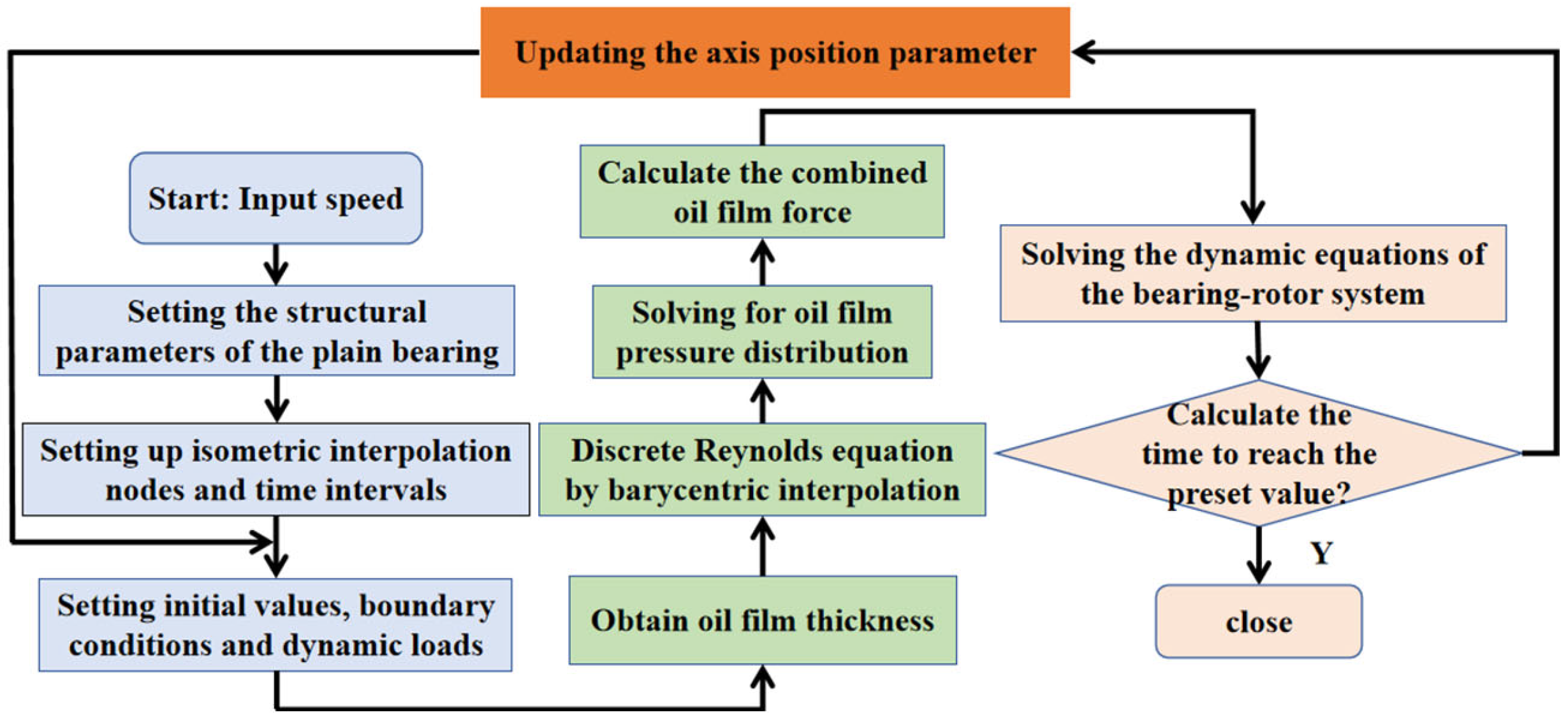
Lubricant density $(\rho$)	876.5 kg/m3

. The flowchart for calculating the dynamic response of the bearing-rotor system is shown in Figure 3.

4.1. Axis Orbit and Dynamic Response

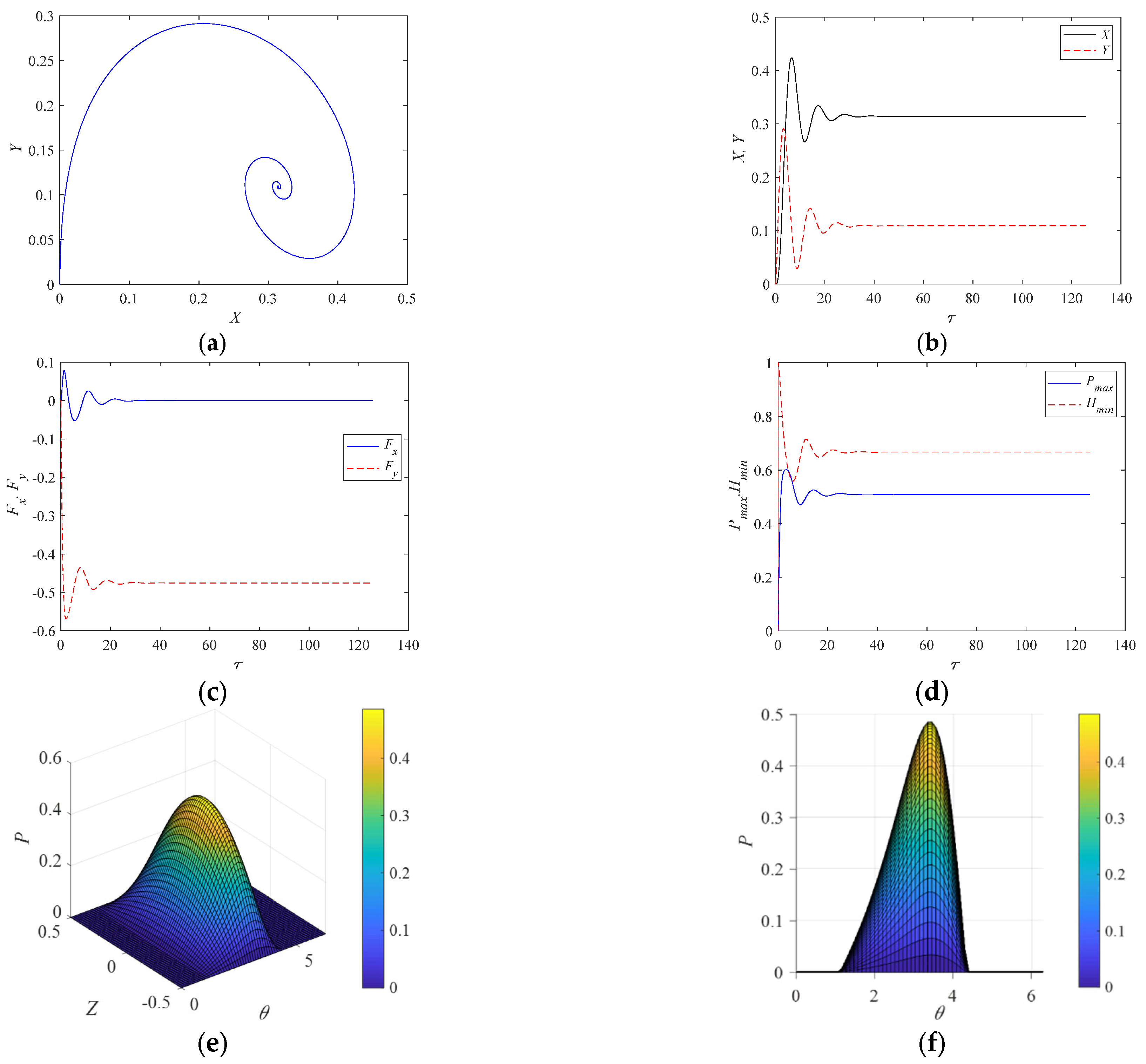
Figure 4 presents the calculation results for a rotor with a mass of M = 20 kg, rotating at a speed of ${\omega }_0=314.159$ r/s, with a computation time of τ = 25π and a time interval of ∆τ = π/100, without considering unbalanced loads and step loads.

Figure 4a illustrates the axis orbit, while Figure 4b–d present the axis displacement response, oil film force components, minimum oil film thickness, and maximum oil film pressure, respectively. It can be observed that in order to balance the gravitational force of the axis, the axis displacement undergoes continuous oscillatory adjustments. Eventually, the gravitational force and the oil film pressure reach equilibrium, and the axis displacement response stabilizes at the equilibrium position with X = 0.301 and Y = 0.1179. From this point onwards, the axis displacement, oil film force components, minimum oil film thickness, and maximum oil film pressure remain constant.

As shown in Figure 4c, the oil film force components are ${\mathrm{F}}_{\mathrm{x}}=0$ and ${\mathrm{F}}_{\mathrm{y}}=-0.4755$. According to the equation of motion (16), it can be calculated that $\eta {\omega }_{0}RL{\left(R/C\right)}^2{F}_y=-196.020019196$, which exactly balances the gravitational force of the axis Mg = 196.0 in magnitude but opposite in direction. At this point, the inertial force is zero, and the bearing is in equilibrium. Figure 4e,f depict the three-dimensional distribution and circumferential distribution of the oil film pressure in the sliding bearing when the rotor reaches a stable operating state.

4.2. The Influence of Rotational Speed on the Stability of Rotor-Bearing Systems

With ${\omega }_0$ as the control parameter, the rotor mass set at M = 20 kg, calculation time τ = 40π, and ∆τ = π/100, while keeping other parameters constant, the dynamic behavior of the bearing-rotor system is analyzed both with and without considering the unbalanced load.

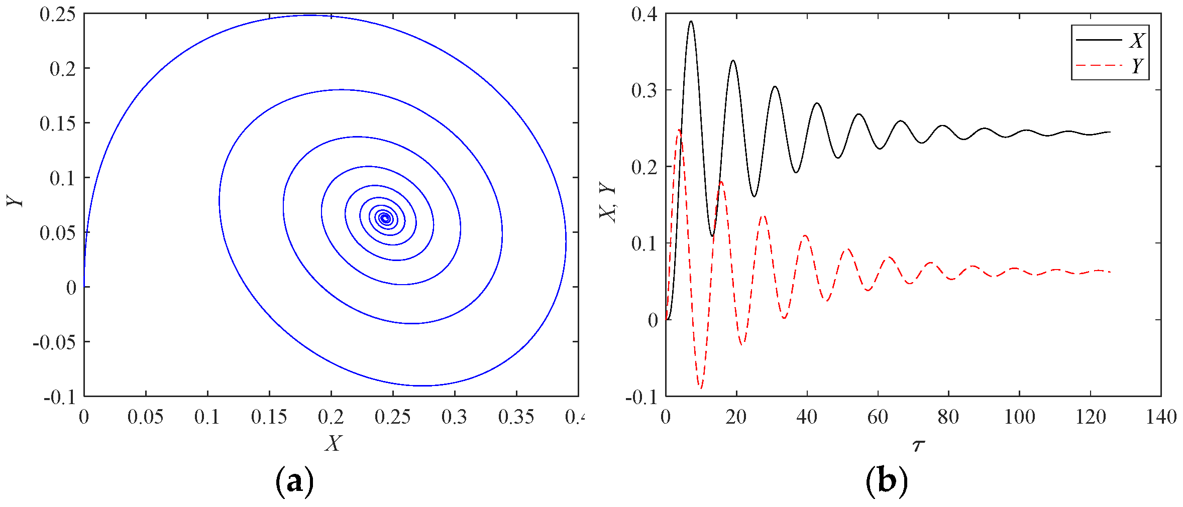
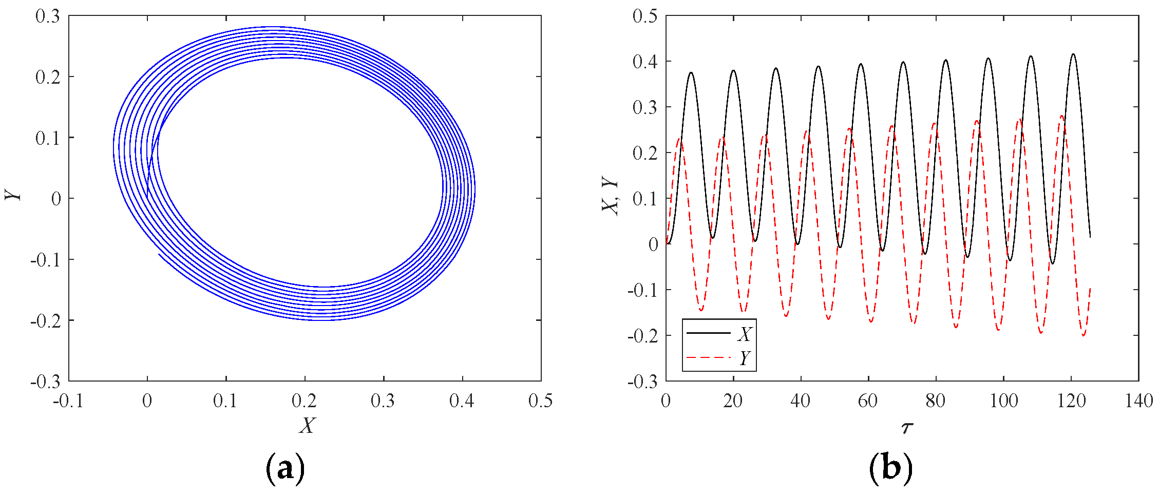
Figure 5, Figure 6, Figure 7 and Figure 8 illustrate the dynamic responses of the bearing-rotor system without considering the unbalanced load, at rotor angular velocities of ${\omega }_0=293.22$ r/s, ${\omega }_0=450.29$ r/s, ${\omega }_0=523.28$ r/s, and ${\omega }_0=528.83$ r/s. Figure 5 shows the dynamic response of the rotor system at ${\omega }_0=293.22 \mathrm{r}/\mathrm{s}$: (a) presents the axis orbit, and (b) displays the axis displacement response. It can be observed that the axis displacement oscillates and then rapidly converges to the static equilibrium position, indicating system stability. 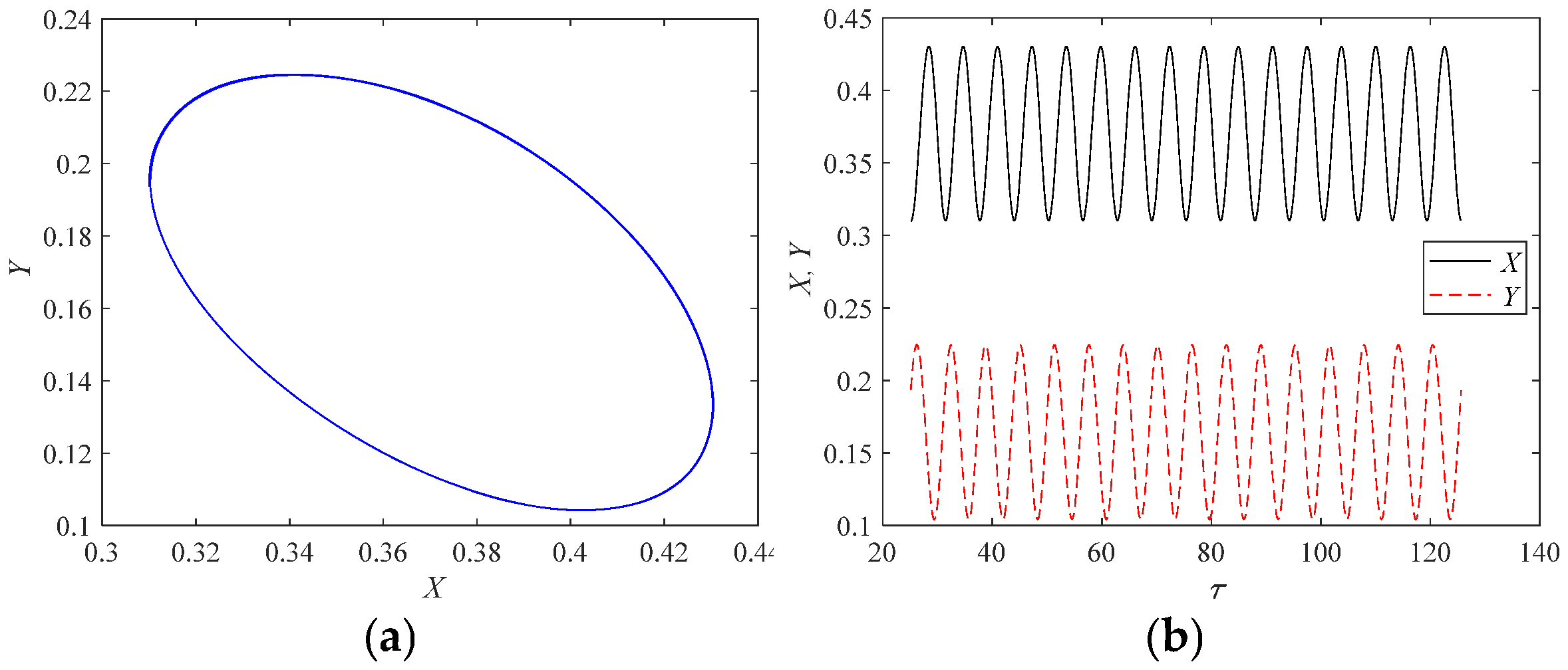As the rotational speed increases, the dynamic response of the rotor system at ${\omega }_0=450.29$ r/s is depicted in Figure 6: (a) shows the axis orbit and (b) presents the axis displacement response. It is evident that the oscillation of the axis displacement gradually decays under damping and eventually converges to the static equilibrium position, indicating that the system ultimately reaches a stable state. With a further increase in rotational speed, the dynamic response of the rotor system at ${\omega }_0=523.28$ r/s is shown in Figure 7: (a) reveals a regular elliptical pattern for the axis orbit and (b) displays a standard sine wave for the axis displacement response, indicating that the system exhibits single-period motion at this stage. When the rotational speed exceeds ${\omega }_0=523.28$ r/s, the dynamic response of the rotor system at ${\omega }_0=528.83$ r/s is illustrated in Figure 8: (a) shows a divergent pattern for the axis orbit, and (b) indicates that the axis displacement response gradually increases over time, suggesting that the bearing-rotor system is in an unstable state.

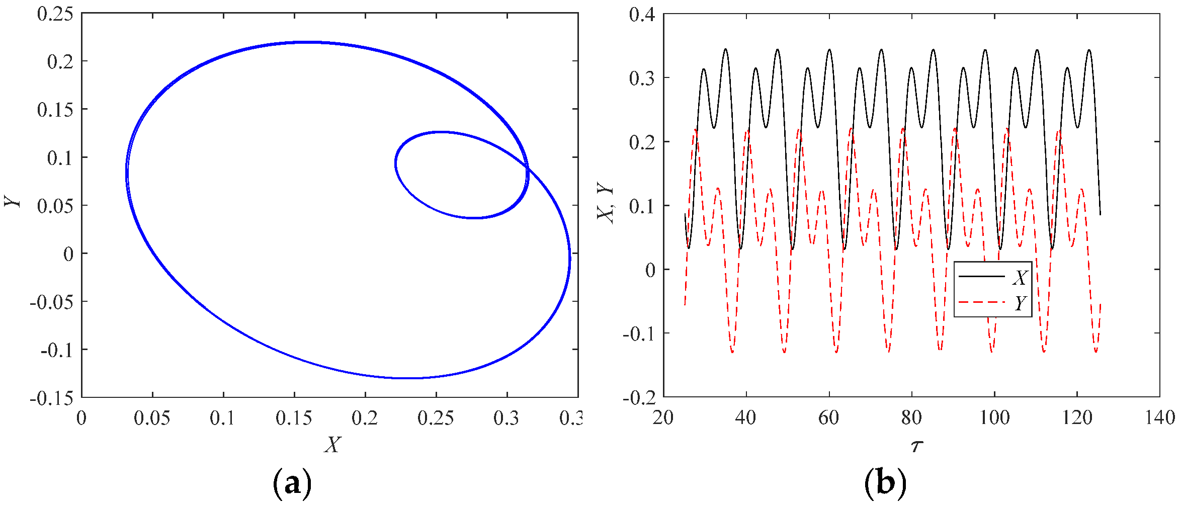
Figure 9 and Figure 10 illustrate the dynamic responses of the bearing-rotor system under the conditions of ${\omega }_0=230.38$ r/s and ${\omega }_0=467.05$ r/s, respectively, considering an imbalance load of ${\mathrm{e}}_{\mathrm{g}}=0.1$ on the rotor. Figure 9 depicts the dynamic response of the rotor system when the rotor angular velocity is ${\omega }_0=230.38$ r/s: Subfigure (a) shows a regular elliptical pattern for the axis orbit. Subfigure (b) presents a standard sinusoidal waveform for the axis displacement response, indicating that the system exhibits single-period motion at this time. As the rotational speed increases, the dynamic response of the rotor system at a rotor angular velocity of ${\omega }_0=467.05 \mathrm{r}/\mathrm{s}$ is shown in Figure 10: Subfigure (a) displays a regular “figure-eight” pattern for the axis orbit. Subfigure (b) demonstrates that the axis displacement response is no longer a curve superimposed by two frequencies. suggesting that the system now exhibits period-doubling motion.

4.3. The Influence of Step Load on the Stability of Rotor-Bearing Systems

When the rotor’s angular velocity reaches the critical speed, the oscillation occur in the axis orbit. At this precise moment, if a step load is skillfully applied to the rotor, it can effectively adjust the equilibrium position of the rotor’s axis, potentially improving the oscillation conditions of the axis. The step load acting on the rotor varies with time τ according to Equation (16).

$$\begin{array}{c}{q}_x\left(\tau \right)=0 \\ q_y\left(\tau \right)=\left\{\begin{array}{c}0,\tau <25\pi \\ 1,\tau \ge 25\pi \end{array}\right.\end{array}$$

(24)

Figure 11 presents the calculation results of the axis orbit, axis displacement, maximum oil film force value $P_{max}$, minimum oil film thickness value $H_{min}$, and oil film resultant forces $F_x$ and $F_y$ over time, before and after applying a step load to the rotor, with the rotor angular velocity at ${\mathsf{\omega }}_0=523.28 \mathrm{r}/\mathrm{s}$ and ignoring the effects of unbalanced loads. When τ < 25π, the axis experiences oscillation, and the axis orbit stabilizes into a closed elliptical path. The maximum oil film force value $P_{max}$ and the oil film resultant force $F_y$ are small, indicating low load-carrying capacity. At τ = 25π, a step load is applied to the rotor in the y-direction. For τ > 25π, due to the effect of the step load, the axis orbit deviates from the elliptical path and stabilizes at a new static equilibrium position. The oscillation disappears, and the bearing returns to a stable state. The absolute values of the maximum oil film force $P_{max}$ and the oil film resultant force $F_y$ increase significantly, enhancing the bearing’s load-carrying capacity.

Figure 12 presents the calculation results of the axis orbit, axis displacement, maximum oil film force value $P_{max}$, minimum oil film thickness value $H_{min}$, and oil film resultant forces $F_x$ and $F_y$ over time, before and after applying a step load to the rotor. With a rotor angular velocity of ${\mathsf{\omega }}_0=466.95 \mathrm{r}/\mathrm{s}$ and an unbalance load of ${\mathrm{e}}_{\mathrm{g}}=0.1$, the axis experiences dual-frequency oscillation when τ < 25π, and the axis orbit stabilizes into a closed “inner Figure 8” path. The maximum oil film force value $P_{max}$ and the oil film resultant force $F_y$ are small, indicating low load-carrying capacity. At τ = 25π, a step load is applied to the rotor in the y-direction. For τ > 25π, due to the effect of the step load, the axis orbit deviates from the “inner Figure 8” path and exhibits small-displacement single-frequency oscillation near a new static equilibrium point, with the axis orbit stabilizing into a small ellipse. The absolute values of the maximum oil film force $P_{max}$ and the oil film resultant force $F_y$ increase significantly, enhancing the bearing’s load-carrying capacity.

In summary, when the rotor’s operating trajectory reaches the critical speed, applying an appropriate step load to the rotor can adjust the position of the axis, which may potentially improve the oscillation condition of the axis.

5. Conclusions

In this paper, a rigid rotor supported by radial journal bearings is taken as the research object. Firstly, nonlinear models for the unsteady oil film force in bearing lubrication and the dynamics of the bearing-rotor system are established. Then, the oil film force model is discretely solved based on the meshless barycentric rational interpolation collocation method, and coupled with the nonlinear equation of motion for the axis orbit, the oil film pressure distribution, dynamic response of the rotor, and the axis orbit are calculated. Furthermore, the dynamic response of the rotor at different rotational speeds is studied both with and without considering unbalanced loads. The results show that rotational speed and unbalanced loads have a significant impact on the stability of rotor motion. Finally, the influence of step loads on rotor motion is analyzed, and it is found that applying appropriate step loads can effectively mitigate the lubricating oil films oscillation conditions, thereby improving the stability of the rotor system. The meshless barycentric rational interpolation collocation method simplifies the modeling of the oil film force model and overcomes the low efficiency of grid-based methods, improving computational efficiency and ease of programming. The results hold significant reference value and practical utility for engineering applications.

(1) When the eccentricity of the rotor mass is ignored, the dynamic response of the rotor is calculated. The amplitude of the axis orbit oscillation is small, gradually decaying to a balanced position, where the load and oil film force reach equilibrium. The rotor then remains stable at this balanced position.

(2) Under the action of unbalanced forces, it is evident that oil film oscillations caused by changes in rotational speed are highly dangerous and must be avoided. To reduce the adverse effects of unbalanced forces, methods such as improving the processing or installation accuracy of the rotor can be adopted to control the unbalance within the specified precision range, thereby enhancing the stability of the rotor system.

(3) By appropriately applying step loads to the rotor, the lubricating oil films oscillation conditions can be reduced and eliminated, effectively improving the stability of the bearing-rotor system. These results have important reference significance and practical value for engineering applications.