Recent Progress of Machine Learning Algorithms for the Oil and Lubricant Industry

Abstract

Machine learning (ML) algorithms have brought about a revolution in many industries where otherwise operation time, cost, and safety would have been compromised. Likewise, in lubrication research, ML has been utilized on many occasions. This review provides an in-depth understanding of seven ML algorithms from a tribological perspective. More specifically, it presents a comprehensive overview of recent advancements in ML applied to lubrication research, organized into four distinct categories. The first category, experimental parameter prediction, highlights the significant contributions of artificial neural networks (ANNs) in accurately forecasting operating conditions related to friction and wear. These predictions offer valuable insights that aid in forensic preparation. Discriminant analysis, Bayesian modeling, and transfer learning approaches have also been used to predict experimental parameters. Second, to predict the lubrication film thickness and identify the lubrication regime, algorithms such as logistic regression and ANN were useful. Such predictions provide up to 99.25% accuracy. Third, to predict the friction and wear for a given experimental condition, support vector machine (SVM), polynomial regression, and ANN offered an accuracy above 93%. Finally, for condition monitoring for bearings, gearboxes, gear trains, and similar critical situations where regular in-person inspection is difficult, Naïve Bayes, SVM, decision trees, and ANN were utilized to predict the safe life of lubricants. This review highlighted these four aspects with state-of-the-art examples and discussed the current situation and projected future possibilities of lubricant design facilitated by ML techniques.

1. Introduction

The modern world is dependent on versatile machinery that is susceptible to continuous friction and wear. As a result, numerous lubricants and additives have been developed to reduce the cost associated with friction and wear [1]. As per the literature, effective use of lubricants could contribute from 1% to 1.55% of the yearly gross domestic product (GDP) of the United States [2,3,4]. Therefore, effective lubrication is extremely important to strengthen the national economy. Lubricants can be categorically divided into three types: liquid, solid, and gaseous [5,6]. Each type has its own application, but overall the purpose is the same: optimizing friction and wear.

Among all lubricants, liquid lubricants have unique functional features that have helped them expand their applicability over many years [7,8]. Solubility, viscosity, heat capacity, wettability, dampening ability, resistance to corrosion, wear, and friction are typical characteristics of liquid lubricants [9,10,11]. Engineers have added solid particles to liquid lubricants and utilized their synergy to reduce friction and wear [12]. Tribologists have also developed superior lubricants that can provide high thermal stability, exhibit low volatility, and have a broad liquid range [13,14]. Therefore, the list of lubricants and their properties has become innumerable nowadays. As a result, it became difficult even for an expert to choose the best lubricant or simply predict the optimum condition for a chosen lubricant without going through a series of trials and errors. In addition, oil analysis is important to maintain the reliability of the equipment and enhance its lifespan. However, using conventional techniques, a data analyst can observe the tribological failure and take steps. But if an earlier prediction could be made, that could minimize the breakdown time. Therefore, tribologists have left their footprints in the computational field and found a wide potential to utilize ML algorithms to predict the optimum lubricant for tribological applications [15].

Machine learning is the study of algorithms that can train and improve themselves through observation. It can be carried out in two ways: (1) supervised learning and (2) unsupervised learning. Both of these types have their pros and cons. As a result, they need to be chosen wisely. Due to the complexity of parameters and methods, computer scientists and tribologists are working together to develop unique tools to predict optimum lubricants and optimum parameters to reach superior performance. Therefore, this approach’s success opens up wide potential to minimize the time and money associated with trial and error, which could strengthen the economy to a great extent [15]. At the current status quo, many tribological studies are devoted to the estimation of the marginal life of lubricants [16,17,18,19]. In practice, the prediction of the limit state for a lubricant is dependent on the manufacturer’s recommendation. When a pre-estimated service life is finished, an oil change is needed. However, the actual health of oil might be better to go on or could be already much worse even before the pre-estimated timeline. Therefore, to optimize the usage of lubricants, continuous monitoring of oil is a strong tool to save machine life and maintenance costs. By monitoring the performance of a lubrication system in real time, it is possible to detect potential issues before they become more serious problems. This can improve the reliability of the lubricants and the performance of the equipment. Therefore, with the development of accurate and efficient models, ML is poised to revolutionize the industry in the coming years [15]. Companies that adopt these technologies will be better positioned to deliver high-performance lubrication solutions that are optimized for specific applications while also reducing downtime and maintenance costs.

Although there is a lot of hype about ML, the available research on this ML perspective for lubrication is scattered. There is a necessity for a review article in this field focusing on different algorithms for researchers to understand and pursue a suitable approach. In this review, nearly 100 scientific journals have been studied to infer current progression and project future path lines for this growing area. Also, this article will be helpful for a tribologist to understand the basics of ML in order to probe its advantages for lubricant selection. This review will provide state-of-the-art insight into ML approaches for lubrication research.

2. Machine Learning

Machine learning could be simply addressed as a computer program that can learn from experience (“E”), with respect to some tasks (“T”), and performance measures (“P”). As per Tom Mitchell, the performance of ML at tasks in “T”, as measured by “P” improves with experience “E” [20]. ML is a subset of artificial intelligence (AI), which helps computers act without explicit programming and instead utilizes the concept of statistics. ML has been widely utilized to find data patterns to make predictions. Nowadays, ML has advanced from pattern recognition studies and is capable of focusing on the recognition of patterns and regularities in data [21].

2.1. Machine Learning Types and Processes

Machine learning techniques can be categorically divided into supervised learning and unsupervised learning [22,23]. Each of these types consists of different processes and algorithms, as shown in Figure 1.

In the case of supervised learning, the model has access to both the training data and their labels, and the model can be trained on the labeled data to perform prediction tasks on any unseen data. The supervised learning task can be formulated as a classification or a regression problem [24]. Classification provides discrete-valued output. It is helpful to predict a characterization for a particular case; for a naive example, machine learning in tribology can predict if wear is coming from a specific type of coated surface or an uncoated surface, which is a discrete-valued output [25].

Regression, on the other hand, provides a continuous numerical value. It is helpful to estimate any relationship between variables. Some of the common regression algorithms are linear regression and logistic regression, to name a few. One example of regression could be the investigation of the relationship between the coefficient of friction (COF) and surface roughness in sliding contact [26,27]. For instance, let us consider a study where different sample surfaces with varying roughness values are subjected to sliding against a counter material. The COF is measured under controlled conditions, and the corresponding surface roughness parameters (Ra, Rq, Rsk, and Rku) are quantified for each sample. A regression analysis could then be performed to determine the correlation between the COF and surface roughness, allowing for the formulation of a predictive model. Such a model could help estimate the friction behavior of similar materials with known surface roughness, aiding in the design and optimization of tribological systems.

For unsupervised learning, no labeled data is provided to the model; rather, an unlabeled data set is fed, and the capabilities of the model are utilized to find the hidden structures in the dataset. Under the unsupervised learning category, cluster analysis is helpful to group a similar set of objects in one group while grouping another set of similar objects in another group. The wear particle data obtained from the lubricated system could be analyzed using this technique. Clustering can form distinct clusters of data that share similarities [28]. Such clustering can provide insights into the wear mechanisms, lubricant effectiveness, or the presence of any irregular wear conditions.

2.2. Machine Learning Algorithms

There are multiple algorithms available to utilize the characterization of a dataset. Each such algorithm needs a unique approach to learning. The choice of one algorithm for favoring a particular benefit could cause a tradeoff of other benefits, including accuracy, complexity, and speed [24]. Therefore, the success of an algorithm depends on the specific nature of the problem, its complexity, cost, and often trial and error.

Currently, there are different platforms to utilize ML algorithms, such as Matlab, Python, C, and C++, to name a few. In Figure 1, different algorithms are presented that are compatible with the Matlab platform [15].

2.3. Explored Machine Learning Algorithms

Machine learning is a process that involves computer programs using software such as MATLAB and Python and needs to be structured following some algorithms. Scientists have explored many fundamental algorithms for lubrication, and a few of them have repeatedly appeared in tribological studies, such as linear regression, logistic regression, support vector machines, discriminant analysis, Naïve Bayes, decision trees, and artificial neural networks. The mathematical modeling of these seven algorithms with relevant tribological examples is summarized here.

2.3.1. Linear Regression

Regression analysis is a widely used technique to analyze multifactor data [29]. The basic idea behind linear regression is to get a line that best describes the relationship between the input and output variables. For example, if x represents an experimental time and y represents a wear volume, then as shown in Figure 2, the straight-line equation relating these two variables could be as follows: where ${\beta }_0$ is the intercept and ${\beta }_1$ is the slope.

$$h\left(x\right)={\beta }_0+{\beta }_1\ast x$$

(1)

Here, h(x) is called the hypothesis function that is used to approximate the target variable (i.e., the wear volume here). By defining an objective function or cost function, computer scientists try to minimize the error between the obtained line and the actual data points. If y is the actual output variable and there are m total training samples, we can write,

$$cost\left({\beta }_0,{\beta }_1\right)=\frac{1}{2}{\displaystyle \sum }_{i=1}^m{\left(h\left(x^{\left(i\right)}\right)-y^{\left(i\right)}\right)}^2$$

(2)

To estimate the parameter values (${\beta }_0$ and ${\beta }_1$) so that the line best fits the data, the cost function needs to be minimized. Researchers use a gradient descent algorithm to minimize the cost function and find the best set of parameters. The multiple linear regression model is used in the case of more than one input variable [30]. There are different variations of linear regression, such as Lasso and Ridge regression, to ensure the generalizability of the model [31].

2.3.2. Logistic Regression

Logistic Regression is a classification algorithm that estimates the probability that a certain data point belongs to a particular class. An investigation to classify the lubrication regime of hydrodynamic journal bearings was carried out using logistic regression [32]. Logistic regression follows a similar learning principle to linear regression. However, unlike linear regression, the output variable is binary, and thus, the input to the output mapping goes through a non-linear transformation called the sigmoid function to make a binary prediction. To illustrate, let us assume we want to fit the data with our hypothesis function h(x), where

$$h\left(x\right)=sigmoid\left({\beta }_0+{\beta }_1\ast x\right)$$

(3)

The sigmoid function can transform any real-numbered value into a range between 0 and 1, which makes it a powerful choice of transformation in classification algorithms. For example, in Figure 3, if $x\to \infty$, then $sigmoid\left(x\right)\to 1$, and if $x\to -\infty$, then $sigmoid\left(x\right)\to 0$. The sigmoid function is defined as

$$sigmoid\left(z\right)=\frac{1}{1+e^{-z} }$$

(4)

Therefore, we obtain

$$h\left(x\right)=\frac{1}{1+e^{-{\beta }_0-{\beta }_1\ast x} }$$

(5)

Here, the cost function is derived using the maximum log-likelihood method.

$$cost\left({\beta }_0,{\beta }_1\right)=\frac{1}{2}{\displaystyle \sum }_{i=1}^m{y}^{\left(i\right)}\log h\left(x^{\left(i\right)}\right)+\left(1-y^{\left(i\right)}\right)\log \left(1-h\left(x^{\left(i\right)}\right)\right)$$

(6)

In a similar way to linear regression, the gradient descent method is used to minimize the cost function and achieve the right set of parameters [33,34].

2.3.3. Support Vector Machines (SVM)

Support vector machines (SVM) are one type of ML algorithm that analyzes data for supervised learning. SVM provides a sorted data map with two groups, with some margins to the farthest possibility. This algorithm has been widely utilized in text recognition, image classification, and many other scientific applications [35,36]. This algorithm was observed as useful for the oil and gas exploration phase of the hydrocarbon industry [37]. It was reported that for hydrocarbon reservoir prediction, the SVM classification method was more suitable than expert judgment or filter approaches [37]. Especially for relatively complex problems, SVM was proven to be more suitable. A similar technique could be useful in tribology for predicting any cracks or irregularities on a material surface. Such a prediction would help to estimate the necessity of additional lubricants.

SVM was first invented in 1992, and over the last thirty years, it has become one of the most powerful ML algorithms [38]. The basic intuition behind the SVM is to build a separating hyperplane in an optimized way to create the maximum margin between two classes.

Let’s assume that in Figure 4, our separating hyperplane forms the following equation:

$$h\left(x\right)=g\left({\beta }_0+{\beta }_1\ast x\right)$$

(7)

However, in most cases, we deal with more than one input variable. So, we can think of $x$ as an n-dimensional vector, where, $x=\left[x_1,x_2,\dots ,x_n\right]$. Here w and b can be defined as model parameters, where, $w=\left[w_1,w_2,\dots ,w_n,\right]$, and b is the intercept term. Therefore, the equation can be rewritten as:

$$h_{w,b}=g\left(w^{T}x+b\right)$$

(8)

Unlike the logistic regression, our target variable $y \in \left\{-1, 1\right\}$. So, we define $g\left(z\right)=1$, if $z \ge 0$, and $g\left(z\right)=-1$ otherwise. In SVM, the concept of maximum margin comes into play. The margin is defined as the closest distance from a data point to the hyperplane. It can be derived mathematically:

$$margin,m=\frac{1}{\Vert w\Vert }$$

(9)

If there are m training examples, the constrained optimization problem of SVM can be written as:

$$\underset{w,b}{minimize}\frac{1}{2}{\Vert w\Vert }^2$$

(10)

$$subject to : y_i\left(w^T{x}_i+b\right) \ge 1,i=1,\dots ,m$$

(11)

There can be non-separable cases where positive and negative examples overlap. Therefore, the soft margin is used by introducing C and $\gamma$ parameters. The parameter C determines the trade-off between the misclassification of training examples and the simplicity of the decision boundary, while the $\gamma$ parameter determines the influence of individual training examples on the decision boundary. Different kernels can be used to learn the SVM in high-dimensional feature space, namely polynomial, gaussian, and radial basis function kernels [39].

2.3.4. Discriminant Analysis

Discriminant analysis is a statistical technique that can differentiate between two or more groups of objects while simultaneously taking several variables into account [40]. This technique was first developed by Fischer in 1936. Discriminant analysis has been used in anthropology, biology, criminology, and political science. Recently, some expeditions on tribology have been carried out with this analysis [41].

The main intuition behind a discriminant analysis (linear) is to find a hyperplane where the projection of the classes will have maximum separability, as shown in Figure 5. Let us assume that the projection of data point X onto the line is y, where $X=\left[x_1,x_2,\dots ,x_m\right]$, and the projection vector $W=\left[w_1,w_2,\dots ,w_m\right]$. We can write

$$y=W^{T}X$$

(12)

Now, if the mean of the features (X) in classes 1 and 2 is ${\mu }_1$ and ${\mu }_2$, and the mean of the projections (y) in classes 1 and 2 are ${\tilde{\mu }}_1$ and ${\tilde{\mu }}_2$,

$${\mu }_c=\frac{1}{N_c}{\displaystyle \sum }_{x\in c}X$$

(13)

$${\tilde{\mu }}_c=W^T{\mu }_c$$

(14)

From that, we define scatter as the sum of square differences between the projected samples and their class mean. Hence, the scatter for class c can be written as:

$${\tilde{S}}_c^2={\displaystyle \sum }_{x ϵ c}{\left(y-{\tilde{\mu }}_c\right)}^2$$

(15)

According to Fisher’s linear discriminant, the objective function can be defined as:

$$J\left(W\right)=\frac{{\left|{\tilde{\mu }}_1-{\tilde{\mu }}_2\right|}^2}{{\tilde{S}}_1^2+{\tilde{S}}_2^2}$$

(16)

Maximizing J ensures that we find a projection line where projections of the same class are in the closest proximity and their means are at the farthest distance.

2.3.5. Naïve Bayes

Naive Bayes is a simple classification technique that utilizes Bayes’ rule along with a string assumption depicting that the attributes are conditionally independent given the class [42]. Naive Bayes has been widely used due to its many desirable features. Sreenath et al. [43] implemented the Naive Bayes algorithm to monitor the failure mode of a gearbox.

According to Bayes theorem, we can write:

$$P\left(H|D\right)=\frac{P\left(H|D\right)P\left(h\right)}{P\left(D\right)}$$

(17)

where

• $P\left(h\right)$ is the probability that a hypothesis is true, irrespective of the data;
• $P\left(D\right)$ is the prior, the overall probability of the data being observed irrespective of the hypothesis;
• $P\left(D|H\right)$ is the probability that the data will be observed if the hypothesis is true;
• $P(H|D)$ is the probability that the hypothesis is true, given the data being observed (posterior).

In Naive Bayes, we first calculate the prior probabilities for given classes. Then the conditional probability of the attributes given the class labels is computed. All these values are used to compute the posterior. We pick the class (the hypothesis) with the maximum posterior, which is also known as the Maximum Posteriori (MAP) decision rule.

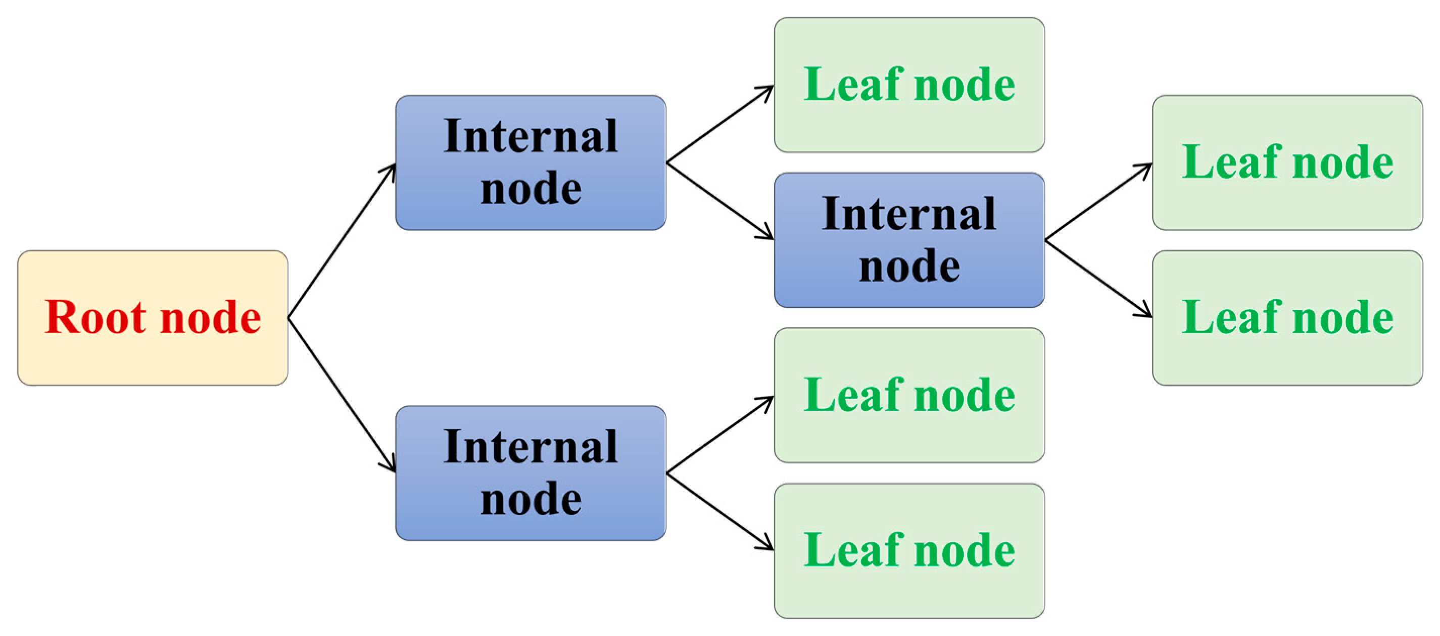
2.3.6. Decision Trees

A Decision Tree is a non-parametric learning algorithm that works by splitting the dataset based on different conditions. This algorithm helps to model the consequences of possible decisions in the context of any outcome or event [44]. Decision tree classification was utilized in lubricant condition monitoring for generating the model for predicting wear conditions of equipment using UOA (used oil analysis), wear particle data, and failure data [45]. Furthermore, it has been used for classifying oil samples, and fault detection [43]. However, despite its flexibility, this model can be sensitive to missing values and outliers.

The Decision Tree works in a tree-like structure, where the topmost node is known as the root (Figure 6). The root is an attribute selected by measuring the information gain, and the feature with the maximum information gain is selected as the root node. The internal nodes are the rest of the features. The branch represents the decision rule, and the leaf nodes (nodes without any children) denote the decision.

2.3.7. Artificial Neural Network (ANN)

An artificial neural network (ANN) is capable of creating models using interconnected mathematical nodes [46,47]. As such, ANN can imitate some abilities of the human brain and probe the advantages of parallel processing, noise immunity, strong fault tolerance, and good memorization [48,49,50]. ANN can learn from samples and explore those samples to realize the relationships between the inputs and results. Therefore, ANN is very suitable for treating nonlinear and complex tribological problems that cannot be solved using traditional physical theories or regular mathematical approaches. The basic step of an ANN is presented in the below picture (Figure 7), where an artificial neural network scheme is shown for fuel consumption prediction based on various engine parameters such as torque, speed, intake air pressure, and EGR%. In a similar fashion, lubrication research was facilitated by ANN to predict lubricant performance or the need for maintenance by analyzing input parameters of the tribological system [51].

A neural network provides a layered representation of the input features in the latent space, with hidden layers and their corresponding activation functions. Activation functions are used to add non-linearity to the neural network.

Let us assume a dataset with n examples has three input features $x_1,x_2,x_3$, and corresponding outputs $\widehat{x_1}, \widehat{x_2},\widehat{x_3}$. The mathematical notation, $a_i{}^{\left(j\right)}$ denotes the neuron in the ith unit of the jth layer. In Figure 8, the first layer is the input layer, which is defined as a vector a⁽¹⁾. All the internal layers other than the final layer are called hidden layers. The first (and only) hidden layer a⁽²⁾ is mapped from the input layer by some weights. The final layer is obtained in the same way and then transformed into a regression or classification setting. It uses a backpropagation algorithm to learn from the error, which is an algorithm to find the gradient required to estimate the weights of the ANN. Backpropagation was first introduced in 1970 but brought to light by Rumelhart et al. in 1986 [53,54]. To introduce non-linearity, the nodes of the layers go through further transformation by an activation function. Depending on the specific problem at hand, the choice of activation function includes sigmoid, tanh, ReLU, and LeakyRelu [43].

As such, for layer 2, the following set of equations can be derived:

$$a_1{}^{\left(2\right)}=g\left({\theta }_{10}^{\left(1\right)}{x}_0+{\theta }_{11}^{\left(1\right)}{x}_1+{\theta }_{12}^{\left(1\right)}{x}_2+{\theta }_{13}^{\left(1\right)}{x}_3\right)$$

(18)

$$a_2{}^{\left(2\right)}=g\left({\theta }_{20}^{\left(1\right)}{x}_0+{\theta }_{21}^{\left(1\right)}{x}_1+{\theta }_{22}^{\left(1\right)}{x}_2+{\theta }_{23}^{\left(1\right)}{x}_3\right)$$

(19)

$$h_{\theta }\left(x\right)=a_1{}^{\left(3\right)}=g\left({\theta }_{10}^{\left(2\right)}{a}_0^{\left(2\right)}+{\theta }_{11}^{\left(2\right)}{a}_1^{\left(2\right)}+{\theta }_{12}^{\left(2\right)}{a}_2^{\left(2\right)}\right)$$

(20)

Here, $\theta$ with different subscripts and superscripts denote the weights. For example, ${\theta }_{ij}^{\left(k\right)}$ denotes the connection weight from the $j$th unit of the $k$th layer to the $i$th unit of ${\left(k+1\right)}^{}$th layer. $x_0$ and $a_0$ denotes the bias terms, and activation is applied through g(.). This process is also called forward propagation (FP). If the dataset has m examples and there are K classes, the cost function can be written as:

$$J\left(\theta \right)=-\frac{1}{m}\left[{\displaystyle \sum }_{i=1}^m{\displaystyle \sum }_{k=1}^K{y}_k^{\left(i\right)}\log {\left(h_{\theta }\left(x^{\left(i\right)}\right)\right)}_k+\left(1-y_k^{\left(i\right)}\right)\log {\left(1-h_{\theta }\left(x^{\left(i\right)}\right)\right)}_k\right]$$

(21)

Using backpropagation, the $\theta$ values are updated with every iteration. The gradient descent algorithm ensures that we find the best set of $\theta$ so as to minimize the cost function.

There are many variations of ANN based on the nature of the task. A few popular algorithms include the Recurrent Neural Network (RNN), Convolutional Neural Network (CNN), and Generative Adversarial Network (GAN), etc. [55,56,57].

3. Application of Machine Learning Algorithms for the Lubricant Industry

The lubricant industry is heading towards automation through condition monitoring and useful life prediction. This shift is not only happening on the experimental side to choose a lubricant; rather, it starts with the extraction of the crude oil from the oil bore [58]. The geological data and drill bit condition monitoring were a primary focus for safe oil extraction. When the crude oil is purified and assigned as lubricants, monitoring is very important to ensure a safe operation for the machine with minimum breakdown. For that, the condition of the lubricant is critical. In addition, at the design phase, the prediction of COF and wear is important to avoid unwanted machine breakdown due to lubrication failure. If the algorithm is trained well, it will predict with higher accuracy, which would be beneficial to designing lubricants with superior qualities. In addition, there have been studies where experimental parameter prediction was a key concern to identify failure conditions. Also, ML algorithms have been utilized for film thickness prediction, which dictates lubricant performance significantly. Overall, the recent progress of ML algorithms for lubrication could be segmented into the following four categories:

• Predicting experimental parameters;
• Predicting film thickness;
• Predicting COF and wear;
• Lubricant condition monitoring.

Each of these categories is discussed in the following sub-sections with a state-of-the-art literature review in tabulated format.

3.1. Predicting Experimental Parameters

Experimental parameter prediction is an important aspect where ML could be utilized. In a few earlier expeditions, wear profiles were inspected and trained against their operating conditions in order to enable the algorithm to predict the experimental conditions for any similar wear profile. This prediction is important because it can tell if any experimental condition has gone wrong. If there is significant wear observed, then the prediction can illustrate the condition behind that wear so that the operator can improvise such extreme conditions quickly to minimize that condition deliberately. Also, performing tests under critical conditions might be more convenient for computer simulation than real experiments.

In the recent past, Gong et al. [59] proposed an approach for simulating the tribochemistry, wear, and stress of a general fully formulated oil and found that tribofilm growth can be promoted by temperature and shear. Information from such simulations could be helpful in training ML models to predict experimental conditions. Also, molecular dynamic simulation can help predict the lubricant’s performance and evaluate its lubrication mechanisms. These techniques have been proven helpful to complement experimental observation to evaluate lubricant performance to some extent. Therefore, parameters from simulations are often used as descriptors to evaluate lubricant performance [60]. In

Table 1. Predicting experimental parameters using ML techniques.

Applied Algorithm	Input Parameters/Descriptors	Involved Lubricants	Remarks	Ref.
Multilayer neural network	Four particle descriptors were used- Representative diameter (0.3 µm to 21 µm) Elongation (1 to 4.7) Roundness (1.1 to 6.5) Reflectivity (0.05–0.92)	Paraffin oil H60 H60 with 0.1 wt.% steric acid H60 with 1.0 wt.% TCP H60 with 0.5 wt.% DBDS H60 with 1.0 wt.% ZndTP	Data was taken from pin-on-disk experiments under 58.8 N and 176 N loads. The wear particle features observed from the microscopic images were analyzed using ML to predict the unknown experimental conditions.	[61]
Fuzzy kohonen neural network, multi-layer perception with backpropagation	Six types of wear particles were analyzed: rubbing, cutting, spherical, laminar, fatigue chunk, and severe sliding. Wear particles were characterized based on: Area, length, roundness, fiber dimension, fractal dimension, Height aspect ratio (HAR), Average roughness (Ra), RMS roughness (Rq), and spectral moment analysis (γ2).	N/A	Six common types of metallic wear were studied using three-dimensional images obtained from laser scanning confocal microscopy. This study showed a way that a neural network could be effectively implemented to classify wear particles.	[62]
Discriminant analysis	Two types of markers were used- Macro (additive elements Ca, Zn, P) Trace (wear metal elements of Ag, Al, Ba, Cd, Cr, Cu, Fe, Mg, Mo, Na, Pb, and Sn)	ZIC A (SK) 5w30 Kixx G1 (GS Caltex) 5w30 HD premium gasoline (Soil) 5w20 ZIC XQ RV/SUV (SK) 5w40 Kixx RV (GS Caltex) 10w40 HD premium diesel (SK) 5w30	Six common automobile gasoline and diesel engine oils were collected from seventy-six sources, analyzed using inductively coupled plasma-optical emission spectrometry (ICP-OES), and then statistically compared. Brand of oil, engine type, and source vehicle type were predicted using ML with 92.1%, 82.9%, and 92.1% accuracy, respectively. This oil analysis would be beneficial for forensic analysis.	[41]
Bayesian modeling and transfer learning approach	Descriptors were selected based on the physical models for estimating dissipation in 2D materials- 1. Lattice constant 2. c/a ratio 3. X-M-X angle 4. Interlayer spacing 5. M-X bond length 6. X-X distance 7. Hexagonal width 8. Covalent radii of M/X atoms 9. In-plane stiffness 10. Cohesive energy per unit cell 11. Thermal conductivity 12. Exciton binding energy 13. Average atomic mass 14. Bandgap energy	Gr BN h-Gr fl-Gr MoS2 MoSe2 MoTe2 NbS2 NbSe2 NbTe2 WS2 WSe2 WTe2 TiS2 TiSe2	Five experimental data sets (from the literature) and ten molecular dynamic simulation data sets of the maximum energy barrier (MEB) of the potential surface energy were obtained. MEB is correlated to intrinsic friction (friction for a crystalline material with no defects) obtained from ten different 2D materials. Less than an 8% difference was observed in MEB values as predicted via the ML model and the PES profiles obtained from the MD simulation.	[60]
Back propagation neural network (BPNN), Generic algorithm (GA)	Content of additives for 25 combinations	Base oil: trimethylolpropane trioleate Additives: AW 34, AW 38, and AW 12 (These were phosphonium-based additives, added up to 1% compared to the base lubricants).	A four-ball test was carried out to compare the results from the experiment and modeling. The content of the three functional additives varied between 0 and 0.7 wt.%, with a total additive wt.% of 1% in the bio-based base lubricant. The content of those additives was used as the input variable for the algorithm. The model was developed by combining the BPNN with GA and provided theoretical guidance for compounding optimization of lubricant additives. The predicted output matched above 90% of the experimental values.	[63]

, a few examples are illustrated where researchers have investigated the experimental conditions against some output results using popular algorithms such as discriminant analysis, Bayesian modeling, and the artificial neural network (ANN).

3.2. Predicting Film Thickness

ML has been implemented to predict the film thickness of lubricants. This is important for gearboxes, where oil lubrication restricts the real contact between gear teeth and reduces friction, heat buildup, vibration, and corrosion. Ali et al. [64] prescribed a lambda ratio (λ) to predict the fatigue life of the gears, where λ is the ratio between film thickness and RMS surface roughness. Basically, the factors that affect the λ ratio are load, temperature, surface roughness, and gear speed [65]. The film thickness could be derived using the following equation [64]:

$$h=\frac{\mathrm{k}{\left({\eta }_0\mathrm{u}\right)}^{0.7}{R}^{0.43}}{{\omega }^{0.13}}\mathsf{\mu }m$$

(22)

Here, η₀ is the dynamic viscosity of the lubricant in Pa·s, k = 1.6 α^0.6 E^0.03, α = pressure-viscosity co-efficient in mm²/N, R = equivalent radius in m, and ω = load applied normal to the line of contact in N/m. It was reported that gears usually operate in the elastohydrodynamic and boundary regimes [64]. In the boundary regime, the film thickness becomes lower, and contact between the tribo-pairs is likely to happen [3,66,67]. Therefore, knowledge about film thickness is very important to design and monitor oil performance. As per their studies, the network simulation conducted by MATLAB Simulink attained 100% success in predicting and classifying at high speed [64].

Table 2. Predicting film thickness and lubrication regime using ML techniques.

Applied Algorithm	Input Parameters/Descriptors	Involved Lubricants	Remarks	Ref.
Neural Network and logistic regression	Six variables in this study were- Specimen speed (rpm) Load (kN) Temperature of oil Friction coefficient Temperature of bearing Contact potential (mV)	Hydrodynamic journal-bearing data was used	A total of 888 high-speed torque measurements were taken in different experiments. Those experiments were carried out on a journal-bearing test rig. Up to 99.25% accuracy was observed for predicting lubricant regime class using an artificial neural network and logistic regression.	[32]
Feed-forward algorithm, Recurrent Elman neural network algorithm, Levenberg-Marquardt back-propagation algorithm	The following information was given as inputs from previous works- RMS roughness Temperature lambda ratio (λ)	Mobil MOBILGEAR 636	MATLAB Simulink was used to run the algorithms to monitor the oil film thickness and detect the lubrication regime for the gearbox. Levenberg–Marquardt’s back-propagation algorithm was used to reduce the error.	[64]
Artificial neural network	Loading conditions were utilized, such as- Vibration, Temperature Torque	Any	The condition of wear and film thickness were predicted using ANN for a gearbox. MATLAB was used to create the simulation model. Hammock–Dowson’s equation was utilized in the model’s development.	[68]

represents individual cases where researchers have investigated the film thickness and highlighted the lubrication regime per the Stribeck curve.

3.3. Predicting COF and Wear

The prediction of COF and wear rate is important from a research and development point of view. A lubricant may provide good performance at one operating condition but may not be effective at other conditions. Predicting their best fit-in situation is important to formulate novel lubricants with superior performances. ML has started to ease this task by helping to predict the COF and wear values for extreme conditions, provided that the algorithm is trained with the data that was obtained from tests previously. In

Table 3. Predicting coefficient of friction and wear for arbitrary experimental conditions using ML techniques.

Applied Algorithm	Input Parameters/Descriptors	Involved Lubricants	Remarks	Ref.
Simple, multivariable, linear, polynomial, and support vector machine regression	The following parameters were calculated under multiple experimental conditions and used as inputs for training the models- Bearing pressure distribution Load carrying capacity friction	Mono-grade SAE 30 Multi-grade SAE 10W-40 Bio lubricant AWS 100	The operating condition was predicted for a thrust bearing with three lubricants. The ASW 100 biolubricant exhibited the lowest friction and better load-carrying capabilities among the three lubricants. The friction prediction using different algorithms varied between 70 and 93%. For example, simple linear regression (79%), simple 2nd order polynomial regression (93%), multivariable linear regression (83%), multivariable 2nd order polynomial regression (93%), and quadratic SVM regression (90%) successfully predict the friction values.	[69]
Bayesian regularization neural network	Molecular connectivity indices were used as the descriptors of 2D BRNN–QSTR models. The descriptors were categorized as: quantum descriptors, 3D descriptors, 2D topological descriptors. Some of the important descriptors were- e IAC_ Mean [70] Balaban indices [71] Wiener index [72]	Thirty-six compounds were tested as additives. Such as- benzoxazole, benzimidazole, benzothiazole, dihydrothiazole piperazine, and piperidine were used as lubricant additives, and their tribological data were examined.	The authors concluded that elements S and P in the lubricant significantly improved tribological properties. Also, minimal carbon chain length is needed in the case of additives. However, extending the carbon chain length might not always be beneficial; rather, there could be a threshold number of carbons in the chain that would facilitate the lowest wear.	[73]
Linear regression	Low orbital energy Dipole moment	Thirty-six lubricant data were used for wear estimation. Among them, 29 groups were used for training purposes whereas 7 groups were used to perform the prediction.	For COF and wear estimation, a standard four-ball tester was used at 1450 rpm over 30 min. A linear regression algorithm was used to predict the wear and COF of seven test lubricants. The database was established in the MySQL database.	[74]
Artificial neural network	Neural network predictor consisted of: one input neuron, ten hidden layer of neurons, and three output neurons with non-linear activation function	Mobil 0W-40	The load-carrying capacity of the journal bearing was investigated with a steel shaft with varying surface textures. The developed neural network was able to learn quickly and predict the load-carrying capacity.	[75]
Feed forward artificial neural network	Four dimensional inputs were- average velocity: 1 to 4 m/s, slide roll ratio (SRR): 2–200%, bath temperature: 40–100 °C contact load: 5–28 N	PAO-6	The experiments were carried out on the tribological testing equipment named a mini-traction machine (MTM) using the ball-on-disk method. The friction coefficient was predicted using the feed-forward artificial neural network, which was simulated in MATLAB software.	[76]
Artificial neural network	Seven inputs from the lubricant properties were: Kinematic viscosity Viscosity index Saponification value Acid value Flash point Pour point Iodine value Inputs taken from the machining conditions were: Operational: sliding, cutting, post sliding Time: 5–90 s (increment of 5) RPM: 100, 150, and 200	Jatropha, Pongam, Neem, Mahua, and mineral oil (Servocut 945)	A tool-chip tribometer was used to simulate a similar aspect of a metal-cutting operation with a pool of oil samples. The prediction was made on the surface roughness and COF using artificial neural network for bio-lubricants.	[77]
Artificial neural network	Loading conditions were utilized, such as- Vibration, Temperature torque	-	The condition of wear and film thickness were predicted using ANN for a gearbox. MATLAB was used to create the simulation model. Hammock–Dowson’s equation was utilized in the model’s development.	[68]
Feed forward back propagation algorithm, Artificial neural network	Load, velocity and additive oil rate	Lubricant (Mineral oil, SAE 20W50) with polytetrafluoroethylene (PTFE) based additives at 1, 3, 5, 10, and 15% concentration	Two loads were implemented (153 and 253 N) for rotational speeds of 30, 60, 120, 180, 240, 300, 360, 420, 480, 540, 600, 660, 720, 780, 840, 900, 960, 1020, 1080, 1140, and 1200 rpm. The average COF from three tests was used to train the algorithm, and the artificial neural network reproduced the COF outputs with 98% accuracy.	[78]
Logistic curve	λ ratio $X={\left(1+{\lambda }^k\right)}^{-a}$  $\mathrm{where} k\approx \frac{3}{2} and a\approx \frac{4}{3}$	SAE 10 W-40 XHVI 5.2 Few other oil data from the literature [79,80]	A new equation: $X={\left(1+{\lambda }^k\right)}^{-a}$ Is proposed that enables the simple calculation of the proportion of mixed/boundary friction in a contact as a function of λ ratio. When the X is plotted against λ, it represents a logistic or sigmoid curve. For a varied λ, this curve could be useful to predict friction under boundary and mixed lubrication regimes.	[81]

, several examples have been presented where ML algorithms have been successfully utilized to predict the coefficient of friction and wear.

3.4. Lubricant Condition Monitoring

Lubricant plays an important role in reducing friction, wear, and associated costs in machinery. Therefore, it is crucial to monitor the lubricant’s conditions regularly. In small-scale applications, periodic checks by maintenance technicians can ensure the safe usage of a lubricant. However, on sites such as wind turbines or in space, regular checking might be difficult. Also, the opportunity cost of inspection could be higher if the lubricant condition is monitored periodically by the shutdown of the running machines. In order to reduce these costs, lubrication condition monitoring (LCM) plays a very vital role. Manghai et al. [82] reviewed brake fault monitoring and highlighted the significance of ML in that process. For lubricant fault monitoring, a few classes of parameters hold significance. In

Table 4. Common parameters used in lubrication monitoring (adapted from [21]).

Class	Parameter	Refs.
Physical	Viscosity at 40 °C and 100 °C, Thermal stability, Temperature, Density, Vibration	[83,84,85]
Chemical	Total Base Number (TBN), Total Acid Number (TAN), Flashpoint	[83,84,85]
Additives	Barium(Ba), Boron (B), Calcium (Ca), Magnesium (Mg), Molybdenum (Mo), Phosphorus (P), Sodium (Na), Silicon (Si), Zinc (Zn)	[86,87]
Contamination	Boron (B), Coolant, Soot/carbon, Potassium (K), Silicon (Si), Sodium (Na), Vanadium (V), Water (H2O)	[88,89,90]
Elemental	Aluminum (Al), Chromium (Cr), Copper (Cu), Iron (Fe), Lead (Pb), Nickel (Ni), Silver (Ag), Titanium (Ti), Tin (Sn), Vanadium (V)	[91,92,93,94]

, such parameters have been tabulated for reference.

Continuous lubrication condition monitoring is especially important for large-scale machine tribo-pairs, wind turbine gearsets, and large plants where regular maintenance might be difficult or may interrupt operating hours. Such interruption could lead to a significant reduction in production, and therefore, automatic condition monitoring could be a great tool to implement. In recent years, companies like SKF have offered remote diagnostic services for machinery that help monitor machine health regularly [95]. Schaeffler Group also offers condition monitoring services for customers, where vibration and temperature are used [96]. A vibration and temperature monitoring system involves a set of tools to measure one or more parameters in order to identify changes in the behavior of machinery. The key advantage of such monitoring is that it helps schedule maintenance activities based on predictive analysis. In addition to temperature and vibration, other parameters such as load, material hardness, and lubricant properties also play an important role and can help predict the service life of lubricants. In some recent research articles in this area, ML algorithms such as ANN, decision trees, Naïve Bayes, and SVM have been utilized. In

Table 5. Predicting lubricant life or other critical information using ML techniques.

Applied Algorithm	Input Parameters/Descriptors	Involved Lubricants	Remarks	Ref.
Artificial neural network	-	Solid lubricants	Solid lubricant performance was studied using the artificial neural network technique.	[46]
Artificial neural networks (ANNs)	Vibration signals extracted from rotating parts were utilized to investigate the effect of oil quality on gearboxes.	Energol® GR-XP SyntHetiC (SHC) SPARTAN EP gear oils Gravis SP series Omala Oil 320 EP gear oil	ANN was employed to predict the vibration parameters of the experimental test rig. The wavelet features were extracted from the vibration data of the gearbox, and the gear fault was classified. The results suggest that the proposed RBNN is more predictive than the MNN. On the other hand, the Omala oil 320 was predicted to be reliable for such gearbox applications compared to other oils.	[51]
Short Time Fourier Transform (STFT), Fuzzy-based classification algorithm	Hardness Normal force Lubricant Lubrication interval	Applicable for any lubricant	STFT was used to extract relevant frequencies. Relationship prediction was possible between the physical failure mode and the calculated characteristics.	[97]
Artificial neural networks (ANNs), adaptive neural-based fuzzy inference systems (ANFIS), and fuzzy clustering method (FCM)	Sliding distance (m) Type Load (N) Cooling rate (°C/s) Volume loss (cm3)	Dry condition	Three cooling rates (0.5, 2, and 3 °C/s) were applied on six specimens made from pre-alloyed Astaloy 85 Mo and Distaloy AB powders through the powder metallurgy (PM) method.	[98]
Decision tree, Naïve Bayes	Statistical features were given as the inputs	No lubricant was considered	The vibration signal was monitored from the actual gearbox of the automobile, with simulated fault conditions within the gear and bearings. The fault detection was performed using two algorithms, and classification accuracy was observed at more than 80% for all cases.	[43]
Random Forest (RF)	Gearbox input load moment and force measurement, torque arm displacement and angular misalignment, wind direction and speed, generator mount displacement, generator rotational speed, and blade pitch angle	None	The authors highlight the need for machine learning in wind turbine drivetrain load monitoring. A RF model is employed to determine sensor positions that significantly influence the accuracy of virtual load sensing in wind turbine transmission.	[99]
Artificial neural network	Lubricant properties were used as inputs. Data were observed and feed based after a certain life interval	-	The remaining utilizable life of the lubricants (RULL) was predicted using ANN.	[100]
Artificial Neural Network (ANN)	Bearing shaft temperature, axial load, rotational speed, lubricant volume flow rate Bearing and resistor voltage, temperature and pressure of storage container, and temperature of chamber input	Not disclosed	The authors used the Long Short-Term Memory (LSTM, a variation of ANN) autoencoders to reconstruct time series data without the white etching cracks (WEC) in order to identify the anomalies in the new unseen data based on the reconstruction error.	[101]
ML technique was not used	Oil samples were analyzed by dint of: Viscosity Viscosity index Element analysis Total acid number (TAN)	Poly alfa olefin (PAO) Mineral oil	Wind turbine gearbox oil was monitored, and the degradation was studied.	[102]
Backpropagation feed-forward neural network algorithm	Input parameters were- Laser power Scanning velocity and energy density	The lubricant was not used, rather surface texturing was studied where the output parameters were average roughness (Sa), RMS roughness (Sq), Skewness (Ssk), Kurtosis (Sku)	Surface roughness parameters were predicted using a neural network. Laser surface processing parameters were used to evaluate the obtained surface properties.	[103]
Support Vector Machine (SVM), Real-time audio signal analysis,	The acoustic emission pattern was filtered and used for training the algorithm	CAW33 type 22,205 bearings were used for the experimental tests.	Bearing failure prediction plays an important role in safety. The SVM classifier provided at least 92% mean accuracy.	[104]
Back propagation neural network, Modular neural network, Radial basis neural network	A wide range of inputs was used for each of the three algorithms	Used and unused engine oils	Two types of vehicle engines were used for the analysis of oil quality and performance. The input layer consisted of 1 neuron, whereas the hidden layer consisted of 10 neurons and the output layer consisted of 4 neurons. This research provided helpful information for industrial applications for vehicle oil analysis and fault detection.	[105]
Artificial neural network	Leakage oil quantity and some other parameters were involved	-	The effect of slippers (which enhance the efficiency of axial piston pumps and motors) on lubrication was studied under different surface roughnesses and conditions).	[106]

, lubricant condition monitoring and surface condition prediction techniques are summarized based on the available literature.

4. Future of ML in the Lubrication Industry

Lubricant design and development over the last century were somewhat dependent on trial and error [107]. Now that ML has been introduced in the lubricant industry, future prospects will undoubtedly be influenced by this technique. Lubricant performance depends on the operating conditions, lubricant properties, and material-pair properties. Therefore, there is scope to incorporate a variety of parameters under machine learning other than those that have already been considered. In recent studies, it was observed that friction and wear can be correlated not only to sliding speed, sliding distance, and normal load but also to properties such as hardness, yield strength, tensile strength, and ductility [108]. It is very likely that ML descriptors will incorporate these variables to project COF and wear and may be able to further predict the associated real-time cost of energy due to such interaction.

Moreover, it is known that to reduce friction and wear, lubricant is introduced between tribo pairs, where the shear strength of the lubricant needs to be less than that of the mating surfaces. Otherwise, there will be abrasion due to the lubricants. Therefore, when using additives or solid lubricants, the shear modulus could be an important parameter. Similarly, the hardness of both mating surfaces is critical to determining the adhesive or plowing wear. ML can be utilized to identify correlations between different properties of lubricants, such as film thickness, viscosity, and COF, which can then be used to optimize lubrication performance for specific applications. As such, the use of ML in tribology has initiated a new branch of studies called “Triboinformatics” [109]. Triboinformatics aims to enhance understanding, prediction, and optimization of tribological processes through the utilization of innovative data-driven approaches. It involves the development of models, algorithms, and databases to capture, store, analyze, and visualize tribological data for various applications, such as lubricant design, material selection, and predictive maintenance. For instance, ML can be used to predict the lubrication properties of a specific set of lubricants under different operating conditions and can help determine the most effective lubricant to use for a particular application. Recent trends in ML for the lubrication industry include the development of efficient models that can forecast the performance of lubricants with a high degree of accuracy [110]. These models can be trained using large datasets, which allows for more accurate predictions of the performance of lubricants in real-world applications. Overall, by using ML algorithms, it is possible to gain insights into lubricant properties that could otherwise be difficult to predict and analyze [74,111,112].

In addition to lubricant design, ML can play a significant role in the predictive maintenance of machines and equipment that require lubrication. The analysis of machine data is one of the fastest-growing areas in the industrial Internet of Things (IoT) and data analytics [113]. By analyzing real-time sensor data, machine-learning algorithms can predict when a machine requires lubrication or maintenance. Another exciting prospect of ML in the lubrication industry is its potential to reduce environmental impact. With the growing concern about climate change, companies are looking for ways to reduce their carbon footprint. ML can be used to optimize lubricant use, minimize waste, and reduce the environmental impact of manufacturing processes. By identifying patterns in data and analyzing performance, ML algorithms can optimize lubrication systems to minimize waste and improve efficiency. Furthermore, with the rise of Industry 4.0, the lubrication industry is rapidly moving towards a more connected, digital future [114]. Companies can leverage the vast amounts of data generated by sensors and equipment to optimize performance, reduce costs, and improve quality using ML techniques. As a result, valuable insights into the operations are possible, which not only predict failures but also make data-driven decisions to improve the bottom line.

In summary, ML is transforming the lubrication industry by providing a more accurate and efficient way of designing lubricants, optimizing lubrication systems, predicting maintenance needs, reducing waste, and improving environmental sustainability [115]. As the technology continues to evolve, ML will play a critical role in the future of lubrication, helping companies to remain competitive and reduce their carbon footprint.

5. Conclusions

ML is a field with versatile applications. With supervised and unsupervised umbrella terms, ML holds a wide variety of algorithms, each with its own unique advantages. Therefore, understanding these algorithms is important for tribologists. Along with the discussions on ML algorithms, this review offered the following conclusions:

• ML techniques are being increasingly utilized in the lubrication research and lubrication industry to enhance lubricant design and optimization and predict maintenance needs;
• Various ML algorithms, such as artificial neural networks, support vector machines, and decision trees, have been successfully applied to predict lubricant properties, such as viscosity, COF, and wear, under different operating conditions;
• ML can assist in identifying correlations between lubricant properties and performance, enabling the optimization of lubrication solutions for specific applications;
• From the literature studies, it was observed that SVM, linear regression, and Bayesian regression have been utilized several times, whereas the number of studies involving artificial neural networks is significant. The ANN algorithm has been improvised for all four aspects discussed with significant accuracy;
• The future of ML in the lubrication industry holds great promise, including advancements in lubricant design, predictive maintenance, environmental sustainability, and optimization of manufacturing processes;
• Lubricant condition monitoring is being improved through the use of ML, allowing for real-time analysis of lubricant parameters and early detection of potential issues in lubrication systems;
• By leveraging ML, companies can make data-driven decisions, reduce costs, improve efficiency, and minimize the environmental impact of lubrication processes;
• For experimental condition prediction or lubricant film estimation, ANN showed significant advantages. Moreover, for COF, wear prediction, and lubricant condition monitoring, researchers relied mostly on ANN. It is because of the built-in feature of neural networks, where the input and output layers are separated by various intermediate layers as per the designers’ requirements. Therefore, the future of the lubricant industry’s prediction ability will depend largely on how efficiently tribologists can develop efficient neural networks that can take tribo-informatics to the next level.

In conclusion, this research provided a thorough examination of seven machine learning algorithms applied in the field of tribology. The selection of tribological examples in this review was meticulously based on the specific algorithms employed, ensuring comprehensive coverage of the four discussed categories. It is important to acknowledge that the boundaries set for this review may have excluded certain articles that explore alternative algorithms and other intriguing topics within the broader realm of machine learning in lubrication. Therefore, considering the rapid advancement of this field, there is immense potential for future review articles to delve into those unexplored aspects and provide valuable insights for aspiring machine learning enthusiasts. Overall, this review will be helpful for researchers to understand the machine learning perspective better from a tribological point of view. The incorporation of ML in tribological studies will reduce machine breakdown and operating costs, help reduce carbon emissions, and unlock many possibilities. This will, in turn, help save energy and build a sustainable future.

References

- Spikes, H. Friction modifier additives. Tribol. Lett. 2015, 60, 5. [Google Scholar] [CrossRef]
- Tzanakis, I.; Hadfield, M.; Thomas, B.; Noya, S.; Henshaw, I.; Austen, S. Future perspectives on sustainable tribology. Renew. Sustain. Energy Rev. 2012, 16, 4126–4140. [Google Scholar] [CrossRef]
- Matczak, L.; Johanning, C.; Gil, E.; Guo, H.; Smith, T.W.; Schertzer, M.; Iglesias, P. Effect of cation nature on the lubricating and physicochemical properties of three ionic liquids. Tribol. Int. 2018, 124, 23–33. [Google Scholar] [CrossRef]
- Stern, D.I. Energy and economic growth in the USA: A multivariate approach. Energy Econ. 1993, 15, 137–150. [Google Scholar] [CrossRef]
- Scharf, T.; Prasad, S. Solid lubricants: A review. J. Mater. Sci. 2013, 48, 511–531. [Google Scholar] [CrossRef]
- Ingole, S.P.; Menezes, P.L.; Nosonovsky, M.; Lovell, M.R.; Kailas, S.V. Tribology for Scientists and Engineers: From Basics to Advanced Concepts; Springer: New York, NY, USA, 2013. [Google Scholar]
- Mortier, R.M.; Orszulik, S.T.; Fox, M.F. Chemistry and Technology of Lubricants; Springer: Dordrecht, The Netherlands; Berlin/Heidelberg, Germany; London, UK; New York, NY, USA, 2010; Volume 107115. [Google Scholar]
- Kasar, A.K.; Siddaiah, A.; Menezes, P.L. Multifunctional Bio-Based Lubricants: Synthesis, Properties and Applications; IOP Publishing: Bristol, UK, 2023. [Google Scholar]
- Cai, M.; Yu, Q.; Liu, W.; Zhou, F. Ionic liquid lubricants: When chemistry meets tribology. Chem. Soc. Rev. 2020, 49, 7753–7818. [Google Scholar] [CrossRef]
- Reeves, C.J.; Siddaiah, A.; Menezes, P.L. Ionic liquids: A plausible future of bio-lubricants. J. Bio-Tribo-Corros. 2017, 3, 18. [Google Scholar] [CrossRef]
- Rahman, M.H.; Warneke, H.; Webbert, H.; Rodriguez, J.; Austin, E.; Tokunaga, K.; Rajak, D.K.; Menezes, P.L. Water-Based Lubricants: Development, Properties, and Performances. Lubricants 2021, 9, 73. [Google Scholar] [CrossRef]
- Sikdar, S.; Rahman, M.H.; Menezes, P.L. Synergistic study of solid lubricant nano-additives incorporated in canola oil for enhancing energy efficiency and sustainability. Sustainability 2021, 14, 290. [Google Scholar] [CrossRef]
- Syahir, A.; Zulkifli, N.; Masjuki, H.; Kalam, M.; Alabdulkarem, A.; Gulzar, M.; Khuong, L.; Harith, M. A review on bio-based lubricants and their applications. J. Clean Prod. 2017, 168, 997–1016. [Google Scholar] [CrossRef]
- Rahman, M.H.; Liu, T.; Macias, T.; Misra, M.; Patel, M.; Martini, A.; Menezes, P.L. Physicochemical and tribological comparison of bio-and halogen-based ionic liquid lubricants. J. Mol. Liq. 2023, 369, 120918. [Google Scholar] [CrossRef]
- Rosenkranz, A.; Marian, M.; Profito, F.J.; Aragon, N.; Shah, R. The Use of Artificial Intelligence in Tribology—A Perspective. Lubricants 2021, 9, 2. [Google Scholar] [CrossRef]
- Shram, V.; Agafonov, E.; Lysyannikov, N.; Lysyannikov, A.; Kovaleva, M. Prediction life of lubricants on the analysis of experimental data on their optical density. J. Phys. Conf. Ser. 2019, 1399, 55009. [Google Scholar] [CrossRef]
- Ghaffari, M.A.; Zhang, Y.; Xiao, S. Multiscale modeling and simulation of rolling contact fatigue. Int. J. Fatigue 2018, 108, 9–17. [Google Scholar] [CrossRef]
- Wolak, A. Statistical analysis of HTHS viscosity rating of present-day engine oils. Tribol. Trans. 2019, 62, 34–41. [Google Scholar] [CrossRef]
- Zhu, Y.; Zhao, T.; Jiao, J.; Chen, Z. The lifetime prediction of epoxy resin adhesive based on small-sample data. Eng. Fail. Anal. 2019, 102, 111–122. [Google Scholar] [CrossRef]
- Randerson. Machine Learning Simplified. Available online: https://randerson112358.medium.com/machine-learning-simplified-407caa414386 (accessed on 26 February 2021).
- Wakiru, J.M.; Pintelon, L.; Muchiri, P.N.; Chemweno, P.K. A review on lubricant condition monitoring information analysis for maintenance decision support. Mech. Syst. Signal Process. 2019, 118, 108–132. [Google Scholar] [CrossRef]
- Mitchell, T.M. Machine Learning; Springer Nature: Berlin/Heidelberg, Germany, 1997. [Google Scholar]
- Goodfellow, I.; Bengio, Y.; Courville, A. Machine learning basics. Deep Learn. 2016, 1, 98–164. [Google Scholar]
- Mathworks. Machine Learning in MATLAB. Available online: https://in.mathworks.com/help/stats/machine-learning-in-matlab.html?w.mathworks.com (accessed on 26 February 2021).
- Kang, J.; Niu, Y.; Zhou, Y.; Fan, Y.; Ma, G. Wear Resistance Prediction of AlCoCrFeNi-X (Ti, Cu) High-Entropy Alloy Coatings Based on Machine Learning. Metals 2023, 13, 939. [Google Scholar] [CrossRef]
- Bien, D.X. Predictive modeling of surface roughness in hard turning with rotary cutting tool based on multiple regression analysis, artificial neural network, and genetic programing methods. Proc. Inst. Mech. Eng. Part B J. Eng. Manuf. 2023, 09544054231157112. [Google Scholar] [CrossRef]
- Suresh, P.; Rao, P.V.; Deshmukh, S. A genetic algorithmic approach for optimization of surface roughness prediction model. Int. J. Mach. Tools Manuf. 2002, 42, 675–680. [Google Scholar] [CrossRef]
- Zhao, D.; Yan, J. Performance prediction methodology based on pattern recognition. Signal Process. 2011, 91, 2194–2203. [Google Scholar] [CrossRef]
- Montgomery, D.C.; Peck, E.A.; Vining, G.G. Introduction to Linear Regression Analysis; John Wiley & Sons: Hoboken, NJ, USA, 2021. [Google Scholar]
- Andrews, D.F. A robust method for multiple linear regression. Technometrics 1974, 16, 523–531. [Google Scholar] [CrossRef]
- Tibshirani, R. Regression shrinkage and selection via the lasso. J. R. Stat. Soc. Ser. B 1996, 58, 267–288. [Google Scholar] [CrossRef]
- Moder, J.; Bergmann, P.; Grün, F. Lubrication Regime Classification of Hydrodynamic Journal Bearings by Machine Learning Using Torque Data. Lubricants 2018, 6, 108. [Google Scholar] [CrossRef]
- Nelder, J.A.; Wedderburn, R.W. Generalized linear models. J. R. Stat. Soc. Ser. A 1972, 135, 370–384. [Google Scholar] [CrossRef]
- Ruder, S. An overview of gradient descent optimization algorithms. arXiv 2016, arXiv:1609.04747. [Google Scholar]
- Ben-Hur, A.; Horn, D.; Siegelmann, H.T.; Vapnik, V. Support vector clustering. J. Mach. Learn. Res. 2001, 2, 125–137. [Google Scholar] [CrossRef]
- Li, H.; Liang, Y.; Xu, Q. Support vector machines and its applications in chemistry. Chemom. Intell. Lab. Syst. 2009, 95, 188–198. [Google Scholar] [CrossRef]
- Ccoicca, Y. Applications of support vector machines in the exploratory phase of petroleum and natural gas: A survey. Int. J. Eng. Technol. 2013, 2, 113. [Google Scholar] [CrossRef]
- Boser, B.E.; Guyon, I.M.; Vapnik, V.N. A training algorithm for optimal margin classifiers. In Proceedings of the Fifth Annual Workshop on Computational Learning Theory, Pittsburgh, PN, USA, 27–29 June 1992; pp. 144–152. [Google Scholar]
- Burges, C.J. A tutorial on support vector machines for pattern recognition. Data Min. Knowl. Discov. 1998, 2, 121–167. [Google Scholar] [CrossRef]
- Klecka, W.R.; Iversen, G.R.; Klecka, W.R. Discriminant Analysis; Sage: Newcastle upon Tyne, UK, 1980; Volume 19. [Google Scholar]
- Kim, Y.; Kim, N.Y.; Park, S.Y.; Lee, D.-k.; Lee, J.H. Classification and individualization of used engine oils using elemental composition and discriminant analysis. Forensic Sci. Int. 2013, 230, 58–67. [Google Scholar] [CrossRef]
- Webb, G.I.; Keogh, E.; Miikkulainen, R. Naïve Bayes. Encycl. Mach. Learn. 2010, 15, 713–714. [Google Scholar]
- Sreenath, P.; Praveen Kumare, G.; Pravin, S.; Vikram, K.; Saimurugan, M. Automobile gearbox fault diagnosis using Naive Bayes and decision tree algorithm. Appl. Mech. Mater. 2015, 813, 943–948. [Google Scholar] [CrossRef]
- Ide, D.; Ruike, A.; Kimura, M. Extraction of causalities and rules involved in wear of machinery from lubricating oil analysis data. In Proceedings of the Second International Conference on Digital Information Processing, Data Mining, and Wireless Communications (DIPDMWC2015), Dubai, United Arab Emirates, 28–30 January 2015; p. 16. [Google Scholar]
- Wakiru, J.M. A Decision Tree-Based Classification Framework for Used Oil Analysis Applying Random Forest Feature Selection. 2018. Available online: http://41.89.227.156:8080/xmlui/handle/123456789/748 (accessed on 5 July 2023).
- Li, D.; Lv, R.; Si, G.; You, Y. Hybrid neural network-based prediction model for tribological properties of polyamide6-based friction materials. Polym. Compos. 2017, 38, 1705–1711. [Google Scholar] [CrossRef]
- Hassoun, M.H. Fundamentals of Artificial Neural Networks; MIT Press: Cambridge, MA, USA, 1995. [Google Scholar]
- Sha, W.; Edwards, K. The use of artificial neural networks in materials science based research. Mater. Des. 2007, 28, 1747–1752. [Google Scholar] [CrossRef]
- Guo, Z.; Sha, W. Modelling the correlation between processing parameters and properties of maraging steels using artificial neural network. Comput. Mater. Sci. 2004, 29, 12–28. [Google Scholar] [CrossRef]
- Zhang, Z.; Friedrich, K. Artificial neural networks applied to polymer composites: A review. Compos. Sci. Technol. 2003, 63, 2029–2044. [Google Scholar] [CrossRef]
- Kalkat, M. Investigations on the effect of oil quality on gearboxes using neural network predictors. Ind. Lubr. Tribol. 2015, 67, 99–109. [Google Scholar] [CrossRef]
- Tomanik, E.; Jimenez-Reyes, A.J.; Tomanik, V.; Tormos, B. Machine-Learning-Based Digital Twins for Transient Vehicle Cycles and Their Potential for Predicting Fuel Consumption. Vehicles 2023, 5, 583–604. [Google Scholar] [CrossRef]
- Linnainmaa, S. The Representation of the Cumulative Rounding Error of an Algorithm as a Taylor Expansion of the Local Rounding Errors. Master’s Thesis, University of Helsinki, Helsinki, Finland, 1970. (In Finnish). [Google Scholar]
- Rumelhart, D.E.; Hinton, G.E.; Williams, R.J. Learning representations by back-propagating errors. Nature 1986, 323, 533–536. [Google Scholar] [CrossRef]
- LeCun, Y.; Bottou, L.; Bengio, Y.; Haffner, P. Gradient-based learning applied to document recognition. Proc. IEEE 1998, 86, 2278–2324. [Google Scholar] [CrossRef]
- Rumelhart, D.E.; Hinton, G.E.; Williams, R.J. Learning Internal Representations by Error Propagation; California University San Diego La Jolla Inst for Cognitive Science: La Jolla, CA, USA, 1985. [Google Scholar]
- Goodfellow, I.; Pouget-Abadie, J.; Mirza, M.; Xu, B.; Warde-Farley, D.; Ozair, S.; Courville, A.; Bengio, Y. Generative adversarial networks. Commun. ACM 2020, 63, 139–144. [Google Scholar] [CrossRef]
- Sircar, A.; Yadav, K.; Rayavarapu, K.; Bist, N.; Oza, H. Application of machine learning and artificial intelligence in oil and gas industry. Pet. Res. 2021, 6, 379–391. [Google Scholar] [CrossRef]
- Gong, Y.; Wang, Y.; Ghanbarzadeh, A.; Wang, C.; Ishihara, A.; Tamura, Y.; Neville, A.; Morina, A. Experimental and numerical study on wear characteristics of steel surfaces involving the tribochemistry of a fully formulated oil. Part II: Computational modelling. Tribol. Int. 2023, 177, 107976. [Google Scholar] [CrossRef]
- Baboukani, B.S.; Ye, Z.; Reyes, K.G.; Nalam, P.C. Prediction of Nanoscale Friction for Two-Dimensional Materials Using a Machine Learning Approach. Tribol. Lett. 2020, 68, 57. [Google Scholar] [CrossRef]
- Umeda, A.; Sugimura, J.; Yamamoto, Y. Characterization of wear particles and their relations with sliding conditions. Wear 1998, 216, 220–228. [Google Scholar] [CrossRef]
- Peng, Z.; Kirk, T. Automatic wear-particle classification using neural networks. Tribol. Lett. 1998, 5, 249–257. [Google Scholar] [CrossRef]
- Yu, T.; Yin, P.; Zhang, W.; Song, Y.; Zhang, X. A compounding-model comprising back propagation neural network and genetic algorithm for performance prediction of bio-based lubricant blending with functional additives. Ind. Lubr. Tribol. 2020, 73, 246–252. [Google Scholar] [CrossRef]
- Ali, Y.H.; Abd Rahman, R.; Hamzah, R.I.R. Artificial neural network model for monitoring oil film regime in spur gear based on acoustic emission data. Shock Vib. 2015, 2015, 106945. [Google Scholar] [CrossRef]
- Hamel, M.; Addali, A.; Mba, D. Monitoring oil film regimes with acoustic emission. Proc. Inst. Mech. Eng. Part J J. Eng. Tribol. 2014, 228, 223–231. [Google Scholar] [CrossRef]
- Hamrock, B.J.; Dowson, D. Ball Bearing Lubrication: The Elastohydrodynamics of Elliptical Contacts; ASME: New York, NY, USA, 1981. [Google Scholar]
- Menezes, P.L.; Kailas, S.V. Effect of roughness parameter and grinding angle on coefficient of friction when sliding of Al–Mg alloy over EN8 steel. J. Tribol. 2006, 128, 697–704. [Google Scholar] [CrossRef]
- Sreepradha, C.; Kumari, A.K.; Perumal, A.E.; Panda, R.C.; Harshabardhan, K.; Aribalagan, M. Neural network model for condition monitoring of wear and film thickness in a gearbox. Neural Comput. Appl. 2014, 24, 1943–1952. [Google Scholar] [CrossRef]
- Katsaros, K.P.; Nikolakopoulos, P.G. On the tilting-pad thrust bearings hydrodynamic lubrication under combined numerical and machine learning techniques. Lubr. Sci. 2021, 33, 153–170. [Google Scholar] [CrossRef]
- Bonchev, D. Information Theoretic Indices for Characterization of Chemical Structures; Research Studies Press: Baldock, UK, 1983. [Google Scholar]
- Balaban, A.T. Highly discriminating distance-based topological index. Chem. Phys. Lett. 1982, 89, 399–404. [Google Scholar] [CrossRef]
- Müller, W.; Szymanski, K.; Knop, J.; Trinajstić, N. An algorithm for construction of the molecular distance matrix. J. Comput. Chem. 1987, 8, 170–173. [Google Scholar] [CrossRef]
- Gao, X.; Dai, K.; Wang, Z.; Wang, T.; He, J. Establishing quantitative structure tribo-ability relationship model using Bayesian regularization neural network. Friction 2016, 4, 105–115. [Google Scholar] [CrossRef]
- Jia, D.; Duan, H.; Zhan, S.; Jin, Y.; Cheng, B.; Li, J. Design and development of lubricating material database and research on performance prediction method of machine learning. Sci. Rep. 2019, 9, 20277. [Google Scholar] [CrossRef]
- Si, C. The analysis of the effects of surface texture on the capability of load carriage of journal bearings using neural network. Ind. Lubr. Tribol. 2005, 57, 28–40. [Google Scholar]
- Echávarri Otero, J.; De La Guerra Ochoa, E.; Chacón Tanarro, E.; Lafont Morgado, P.; Díaz Lantada, A.; Munoz-Guijosa, J.; Muñoz Sanz, J. Artificial neural network approach to predict the lubricated friction coefficient. Lubr. Sci. 2014, 26, 141–162. [Google Scholar] [CrossRef]
- Bharadwaj, P.V.; Jeevan, T.; Suvin, P.; Jayaram, S. Prediction of Surface Roughness and Coefficient of Friction Using Artificial Neural Network in Tribotesting of Bio-Lubricants. Appl. Mech. Mater. 2019, 895, 52–57. [Google Scholar] [CrossRef]
- Durak, E.; Salman, Ö.; Kurbanoğlu, C. Analysis of effects of oil additive into friction coefficient variations on journal bearing using artificial neural network. Ind. Lubr. Tribol. 2008, 60, 309–316. [Google Scholar] [CrossRef]
- Dawczyk, J.; Morgan, N.; Russo, J.; Spikes, H. Film thickness and friction of ZDDP tribofilms. Tribol. Lett. 2019, 67, 34. [Google Scholar] [CrossRef]
- Kanazawa, Y.; Sayles, R.S.; Kadiric, A. Film formation and friction in grease lubricated rolling-sliding non-conformal contacts. Tribol. Int. 2017, 109, 505–518. [Google Scholar] [CrossRef]
- Taylor, R.I.; Sherrington, I. A simplified approach to the prediction of mixed and boundary friction. Tribol. Int. 2022, 175, 107836. [Google Scholar] [CrossRef]
- Manghai, A.; Jegadeeshwaran, R.; Sugumaran, V. Brake Fault Diagnosis Through Machine Learning Approaches—A Review. Struct. Durab. Health Monit. 2017, 11, 43. [Google Scholar]
- Ljubas, D.; Krpan, H.; Matanović, I. Influence of engine oils dilution by fuels on their viscosity, flash point and fire point. Naft. Explor. Prod. Process. Petrochem. 2010, 61, 73–79. [Google Scholar]
- Afrand, M.; Najafabadi, K.N.; Sina, N.; Safaei, M.R.; Kherbeet, A.S.; Wongwises, S.; Dahari, M. Prediction of dynamic viscosity of a hybrid nano-lubricant by an optimal artificial neural network. Int. Commun. Heat Mass Transf. 2016, 76, 209–214. [Google Scholar] [CrossRef]
- Kocsis, M.C.; Briggs, T.; Anderson, G. The impact of lubricant volatility, viscosity and detergent chemistry on low speed pre-ignition behavior. SAE Int. J. Engines 2017, 10, 1019–1035. [Google Scholar] [CrossRef]
- Vališ, D.; Žák, L. Oil additives used as indicator and input for preventive maintenance optimisation. In Proceedings of the International Conference on Military Technologies (ICMT) 2015, Brno, Czech Republic, 19–21 May 2015; pp. 1–6. [Google Scholar]
- Dave, V.S.; Popielarczyk, M.; Boyce, H.; Al-Achi, A.; Ike-Amaechi, E.; Hoag, S.W.; Haware, R.V. Lubricant-sensitivity assessment of SPRESS® B820 by near-infrared spectroscopy: A comparison of multivariate methods. J. Pharm. Sci. 2017, 106, 537–545. [Google Scholar] [CrossRef]
- Barker, J.; Cook, S.; Richards, P. Sodium contamination of diesel fuel, its interaction with fuel additives and the resultant effects on filter plugging and injector fouling. SAE Int. J. Fuels Lubr. 2013, 6, 826–838. [Google Scholar] [CrossRef]
- George, S.; Balla, S.; Gautam, V.; Gautam, M. Effect of diesel soot on lubricant oil viscosity. Tribol. Int. 2007, 40, 809–818. [Google Scholar] [CrossRef]
- Prabhakaran, A.; Jagga, C. Condition monitoring of steam turbine-generator through contamination analysis of used lubricating oil. Tribol. Int. 1999, 32, 145–152. [Google Scholar] [CrossRef]
- Kumar, M.; Mukherjee, P.S.; Misra, N.M. Advancement and current status of wear debris analysis for machine condition monitoring: A review. Ind. Lubr. Tribol. 2013, 65, 3–11. [Google Scholar] [CrossRef]
- Cao, W.; Wang, W.J.; Wang, R. Wear trend prediction of gearbox based on oil monitoring technology. Adv. Mater. Res. 2012, 411, 576–579. [Google Scholar] [CrossRef]
- Fan, B.; Li, B.; Feng, S.; Mao, J.; Xie, Y.-B. Modeling and experimental investigations on the relationship between wear debris concentration and wear rate in lubrication systems. Tribol. Int. 2017, 109, 114–123. [Google Scholar] [CrossRef]
- Hu, Y.; Wang, L.; Politis, D.; Masen, M. Development of an interactive friction model for the prediction of lubricant breakdown behaviour during sliding wear. Tribol. Int. 2017, 110, 370–377. [Google Scholar] [CrossRef]
- SKF. Vibration Analysis and Diagnostics. Available online: https://www.skf.com/us/services/condition-based-maintenance/vibration-analysis-and-diagnostics (accessed on 22 June 2023).
- Schaeffler. Schaeffler OPTIME Condition Monitoring. Available online: https://www.schaeffler.com/ (accessed on 22 June 2023).
- Söffker, D.; Rothe, S. New Approaches for Supervision of Systems with Sliding Wear: Fundamental Problems and Experimental Results Using Different Approaches. Appl. Sci. 2017, 7, 843. [Google Scholar] [CrossRef]
- Alambeigi, F.; Khadem, S.M.; Khorsand, H.; Hasan, E.M.S. A comparison of performance of artificial intelligence methods in prediction of dry sliding wear behavior. Int. J. Adv. Manuf. Technol. 2016, 84, 1981–1994. [Google Scholar] [CrossRef]
- Azzam, B.; Schelenz, R.; Jacobs, G. Sensor Screening Methodology for Virtually Sensing Transmission Input Loads of a Wind Turbine Using Machine Learning Techniques and Drivetrain Simulations. Sensors 2022, 22, 3659. [Google Scholar] [CrossRef]
- Sinha, A.; Mukherjee, P.; De, A. Assessment of useful life of lubricants using artificial neural network. Ind. Lubr. Tribol. 2000, 52, 105–109. [Google Scholar] [CrossRef]
- Liu, X.; Azzam, B.; Harzendorf, F.; Kolb, J.; Schelenz, R.; Hameyer, K.; Jacobs, G. Early stage white etching crack identification using artificial neural networks. Forsch. Ing. 2021, 85, 153–163. [Google Scholar] [CrossRef]
- Coronado, D.; Wenske, J. Monitoring the oil of wind-turbine gearboxes: Main degradation indicators and detection methods. Machines 2018, 6, 25. [Google Scholar] [CrossRef]
- Yang, L. Prediction of Surface Texture Parameters Using Machine Learning in Laser Surface Texturing; Rutgers University-School of Graduate Studies: New Brunswick, NJ, USA, 2020. [Google Scholar]
- Marin, F.; Solomon, C.; Marin, M. Bearing failure prediction using audio signal analysis based on SVM algorithms. In Proceedings of the IOP Conference Series: Materials Science and Engineering, Galati, Romania, 11–13 October 2018; p. 012012. [Google Scholar]
- Kalkat, M.; Yıldırım, Ş.; Erkaya, S. Oils quality and performance analysis of vehicle’s engines using radial basis neural networks. Ind. Lubr. Tribol. 2009, 61, 301–310. [Google Scholar] [CrossRef]
- Canbulut, F.; Sinanoğlu, C.; Yildirim, Ş. Neural network analysis of leakage oil quantity in the design of partially hydrostatic slipper bearings. Ind. Lubr. Tribol. 2004, 56, 231–243. [Google Scholar] [CrossRef]
- Tysoe, W.T.; Spencer, N.D. Designing lubricants by artificial intelligence-the sequel. Tribol. Lubr. Technol. 2020, 76, 68–70. [Google Scholar]
- Hasan, M.S.; Kordijazi, A.; Rohatgi, P.K.; Nosonovsky, M. Triboinformatic modeling of dry friction and wear of aluminum base alloys using machine learning algorithms. Tribol. Int. 2021, 161, 107065. [Google Scholar] [CrossRef]
- Hasan, M.S.; Kordijazi, A.; Rohatgi, P.K.; Nosonovsky, M. Triboinformatics approach for friction and wear prediction of Al-graphite composites using machine learning methods. J. Tribol. 2022, 144, 11701. [Google Scholar] [CrossRef]
- Desai, P.S.; Granja, V.; Higgs, C.F., III. Lifetime prediction using a tribology-aware, deep learning-based digital twin of ball bearing-like tribosystems in oil and gas. Processes 2021, 9, 922. [Google Scholar] [CrossRef]
- Zhang, Y.; Xu, X. Machine learning decomposition onset temperature of lubricant additives. J. Mater. Eng. Perform. 2020, 29, 6605–6616. [Google Scholar] [CrossRef]
- Urban, A.; Zhe, J. A microsensor array for diesel engine lubricant monitoring using deep learning with stochastic global optimization. Sens. Actuators A Phys. 2022, 343, 113671. [Google Scholar] [CrossRef]
- Paturi, U.M.R.; Palakurthy, S.T.; Reddy, N. The role of machine learning in tribology: A systematic review. Arch. Comput. Methods Eng. 2023, 30, 1345–1397. [Google Scholar] [CrossRef]
- Paolanti, M.; Romeo, L.; Felicetti, A.; Mancini, A.; Frontoni, E.; Loncarski, J. Machine learning approach for predictive maintenance in industry 4.0. In Proceedings of the 2018 14th IEEE/ASME International Conference on Mechatronic and Embedded Systems and Applications (MESA), Oulu, Finland, 2–4 July 2018; pp. 1–6. [Google Scholar]
- Kasar, A.K.; Hill, P.; Sikdar, S.; Menezes, P.L. Machine learning to develop lubrication strategies. In Multifunctional Bio-Based Lubricants: Synthesis, Properties and Applications; IOP Publishing: Bristol, UK, 2023; pp. 5-1–5-16. [Google Scholar]