Article

Impact of Ad Hoc Post-Processing Parameters on the Lubricant Viscosity Calculated with Equilibrium Molecular Dynamics Simulations

by
Gözdenur Toraman
1,
Toon Verstraelen
2 and
Dieter Fauconnier
1,3,*
1
Soete Laboratory, Ghent University, Technologiepark-Zwijnaarde 46, 9052 Ghent, Belgium
2
Center for Molecular Modeling (CMM), Ghent University, Technologiepark-Zwijnaarde 46, 9052 Ghent, Belgium
3
FlandersMake@UGent, Core Lab MIRO, 9000 Ghent, Belgium
*
Author to whom correspondence should be addressed.
Lubricants 2023, 11(4), 183; https://doi.org/10.3390/lubricants11040183
Submission received: 21 March 2023 / Revised: 13 April 2023 / Accepted: 17 April 2023 / Published: 19 April 2023

Abstract

:
Viscosity is a crucial property of liquid lubricants, and it is theoretically a well-defined quantity in molecular dynamics (MD) simulations. However, no standardized protocol has been defined for calculating this property from equilibrium MD simulations. While best practices do exist, the actual calculation depends on several ad hoc decisions during the post-processing of the raw MD data. A common protocol for calculating the viscosity with equilibrium MD simulations is called the time decomposition method (TDM). Although the TDM attempts to standardize the viscosity calculation using the Green–Kubo method, it still relies on certain empirical rules and subjective user observations, e.g., the plateau region of the Green–Kubo integral or the integration cut-off time. It is known that the TDM works reasonably well for low-viscosity fluids, e.g., at high temperatures. However, modified heuristics have been proposed at high pressures, indicating that no single set of rules works well for all circumstances. This study examines the effect of heuristics and ad hoc decisions on the predicted viscosity of a short, branched lubricant molecule, 2,2,4-trimethylhexane. Equilibrium molecular dynamics simulations were performed at various operating conditions (high pressures and temperatures), followed by post-processing with three levels of uncertainty quantification. A new approach, “Enhanced Bootstrapping”, is introduced to assess the effects of individual ad hoc parameters on the viscosity. The results show a strong linear correlation (with a Pearson correlation coefficient of up to 36%) between the calculated viscosity and an ad hoc TDM parameter, which determines the integration cut-off time, under realistic lubrication conditions, particularly at high pressures. This study reveals that ad hoc decisions can lead to potentially misleading conclusions when the post-processing is performed ambiguously.

Graphical Abstract

1. Introduction

Key machine components which are characterized by heavily loaded non-conformal contacts, such as bearings and gears, ideally operate in the so-called (thermo-)elasto-hydrodynamic (TEHL) lubrication regime. In this specific regime, the surfaces in relative motion are entirely separated by a thin lubricant film (<1 μm), in which the hydrodynamic pressures can increase by several orders of magnitude, typically up to 0.5–3.0 GPa. In addition, high shear rates (> 1   ×   10 8   s 1 ) and high contact temperatures may occur, depending on the slide-to-roll ratio at the contact. The state variables, i.e., pressure, shear rate, and temperature, heavily influence the lubricant properties within the contact conjunction. Due to the extremely high hydrodynamic pressures, the lubricant is locally compressed, resulting in intensified interaction between adjacent molecules. As a consequence, and in addition to the increase in the lubricant density, the lubricant viscosity increases even faster than exponentially (super-Arrhenius piezo-viscous response) after a certain inflection point [1].
The determination of pressure-induced changes in viscosity is a challenging task due to experimental limitations. Especially at pressures above 0.5 GPa, specialized high-pressure viscometers and/or rheometers are required. As a result, several empirical rheological models are commonly used to extrapolate the viscosity to high pressures based on available measurements at low pressures [2,3,4,5,6]. Several studies performed high-pressure characterizations of liquids [7,8]. For example, Bair [7] presented measurements for squalane, which was suggested to be a reference lubricant for EHL, up to 1.2 GPa. However, high-pressure rheological experiments are typically limited to 1.2–1.5 GPa , and the apparatuses for such experiments are costly [9].
Since the experimental determination of lubricant properties at high pressures is quite challenging, the precise constitutive behavior of most lubricants under relevant pressure conditions remains unknown. However, quantifying and assessing changes in the viscosity over a wide range of temperatures and pressures is critical to accurately predicting the performance of a system operating in the TEHL regime [9,10]. In recent decades, molecular dynamics (MD) simulations have been shown to provide a promising computational alternative because such simulations account for all the atomic-scale processes underlying many macroscopic tribological phenomena.
There are two main classes of molecular dynamics (MD) simulations: equilibrium MD (EMD) and non-equilibrium MD (NEMD). Both methods can be used to calculate lubricant viscosity, but both have different strengths and ranges of applicability. NEMD simulations impose relatively high shear rates (typically > 1   ×   10 7   s 1 ) to ensure that the relevant lubricant properties reach a steady state [11]. Although NEMD requires long simulation times to achieve accurate results, it is well-established. The lower shear rates can also be simulated directly, but this requires significantly longer simulation times, extending beyond the nanosecond or even microsecond timescale in extreme cases. As an alternative, viscosity at lower or zero shear rates can be extrapolated empirically [12]. When multiple transport properties are of interest, such as viscosity and thermal conductivity, separate types of NEMD simulation are required. In contrast, all transport properties can be obtained from a single EMD simulation at zero shear rate [11,13]. Several studies have argued that EMD methods provide consistent and reliable estimates as long as convergence issues are handled and post-simulation analysis is performed properly [14,15,16], which is exactly the subject of this paper.

1.1. State-of-the-Art

Several factors determine the accuracy of MD predictions. One of them is the force field that describes the interactions at the atomistic scale. In particular, the prediction of lubricant viscosity at high pressures (generally exceeding 500 MPa) requires accurate force fields as a result of the intensified interactions experienced by lubricant molecules. This accuracy can be increased by re-parameterizing the model for Van der Waals interactions using first-principle techniques, as suggested by Ewen et al. [17]. This can be facilitated by employing machine learning potentials in EMD or NEMD simulations to achieve the accuracy of first-principle techniques [18,19,20].
In addition to force-field approximations, the post-processing of the EMD trajectories affects the calculated viscosity. [13,21] The theoretical foundations of viscosity calculations are well established, but no standardized protocol has been developed that yields consistent results. While the Green–Kubo expression [13,22,23] is more widely used among the two EMD methods (i.e., Green–Kubo and Einstein [13]) for calculating the viscosity of fluids, due to its practical advantages, there is a growing interest in the Einstein methods. For example, the Einstein–Helfand method [24], which calculates the viscosity using the mean square displacements of P α β , has recently been used to rapidly screen the viscosity of lubricant-like molecules [25]. The Green–Kubo method makes use of the autocorrelation of off-diagonal elements of the stress tensor:
A α β ( Δ t ) = P α β ( t + Δ t ) P α β ( t ) t
where Δ t is the time lag and α and β are off-diagonal Cartesian components of the stress tensor. The viscosity is then derived as:
η = lim Δ t η α β ( Δ t ) with η α β ( Δ t ) = V k B T 0 Δ t A α β ( Δ t ) d ( Δ t )
where V is the volume of the system, T is its temperature, and k B is the Boltzmann constant. This expression is valid for any pair of off-diagonal stress components, and it is common to average η α β ( Δ t ) over the three distinct index pairs, which will be referred to as η ( Δ t ) , sometimes denoted as the viscosity running integral [26].
Due to the finite length of the EMD simulations, η can only be approximated: (i) the data to construct the auto-correlation function are limited (averaging over t in Equation (1)) and (ii) the simulation time limits the maximum time lag available to approximate Δ t . As a result, the predicted viscosity depends on the details of the extrapolation, which is a pertinent problem for more complex cases with exceedingly long correlation times. One must realize that naively calculating η α β ( Δ t ) with the largest possible Δ t is unwise. For a fixed simulation time, the auto-correlation function is better resolved for small time lags: As Δ t increases, there are fewer non-overlapping [ t , t + Δ t ] windows and thus fewer independent sample points of P α β ( t + Δ t ) P α β ( t ) in Equation (1). Hence, as time lags increase, A α β ( Δ t ) and η α β ( Δ t ) lose statistical significance. Reliable extrapolations of η α β ( Δ t ) for Δ t must consider the increase in uncertainty as Δ t increases.
Several approaches have been proposed to identify and analyse the relevant part of η ( Δ t ) . In earlier studies, Zhang et al. [27] and Alfe et al. [28] suggested fitting a model to η ( Δ t ) data up to a cut-off time, Δ t cut , which was initially determined by the first root of the auto-correlation function. Other studies estimated viscosity as an average over a certain region of the running integral η ( Δ t ) without determining a cut-off time [14,29]. In their study of imidazolium-based room-temperature ionic liquids, Mondal and Balasubramanian [30] used a much larger cut-off value of 4 n s because of the slow system dynamics of ionic liquids. In a recent study, Carlson et al. [16] recommended including at least the initial 1 / 3 of a simulation to ensure reliable results. Clearly, these studies rely on ad hoc decisions. In 2015, Zhang et al. [26] pointed out how several of these decisions can affect the outcomes of the EMD simulations and provided more objective rules to fix these choices, effectively standardizing the calculation of shear viscosity using the Green–Kubo relation. The main idea of their time decomposition method (TDM) is to replace one expensive, long simulation with multiple shorter ones. These can be carried out in parallel and make it easier to identify the relevant part of η ( Δ t ) . After the introduction of the TDM, the method became increasingly popular and has been successfully applied to systems with lower viscosity, e.g., due to an elevated temperature [26,31,32]. In other words, systems with faster dynamics were preferred, since modeling highly viscous liquids, and in particular piezo-viscous effects, requires extremely long simulations as a result of slower system dynamics. Later, an alternative approach to the TDM was proposed in the study of Heyes et al. [33] by fitting an analytical function (i.e., the sech function) to the stress tensor auto-correlation function.
In recent years, the modeling of lubricant behavior at high pressures occurring in TEHL conditions has increased significantly because of the aforementioned experimental challenges and limitations. In 2018, the 10th Industrial Fluid Properties Simulation Challenge (10th IFPSC: http://fluidproperties.org/10th, accessed on 18 April 2023) was devoted to testing the capabilities of MD simulations for (T)EHL. A short, linear, branched alkane lubricant molecule, 2,2,4-trimethylhexane (C9H 20 ), which has relatively low viscosity, was chosen for computational simplicity. The TDM has been applied in several entries of this challenge [34,35,36]. Zheng et al. [36] used the TDM-GK approach only up to 600 MPa, and the authors reported solidification above 400 MPa. The study of Kondratyuk and Pisarev [34] reported significant under-prediction of the viscosity above 600 MPa, whereas Messerly et al. [35] significantly over-predicted the viscosity. Nevertheless, both studies could accurately predict the viscosity up to 600 MPa. Deviations from the available experimental data could be attributed to the performances of the different force fields used, namely, the Condensed-phase Optimized Molecular Potentials for Atomistic Simulation Studies (COMPASS) [37] and the Mie Potentials for Phase Equilibria (MiPPE) [38,39].
Interestingly, different entries for the 10th IFPSC also modified the original ad hoc decisions in the TDM, such as the number of EMD simulations, the simulation time, and other TDM-specific parameters, e.g., those affecting the cut-off time. (The TDM-specific parameters are defined in the Methods section.) Kondratyuk and Pisarev [34] used 30 EMD trajectories 1 ns long for pressures between 0.1 and 200 MPa with a cut-off time of 100 ps, and  2 ns long individual trajectories for pressures above 200 MPa. At high pressures, the cut-off time was also increased to 300 ps. In the work of Messerly et al. [35], between 40 and 80 independent EMD trajectories were used. A larger number of simulations was preferred at higher pressures. Until 150 MPa, 1 ns long production runs were performed, and the simulation times of individual trajectories were increased up to 96 ns at 1 GPa. The same authors also modified the heuristics for determining the cut-off time in the TDM. The amendments to the original TDM are justified by stating that such changes are necessary to achieve converged results for more viscous systems. In several other studies by Kondratyuk and co-workers [31,40,41], similar improvements to the TDM were proposed.
In 2018, a comprehensive study by Maginn et al. provided “best practices” for calculating self-diffusion coefficients and viscosities from EMD simulations [21]. The importance of clear communication was emphasized, as the implementation of EMD methods requires some user judgment in the post-simulation analysis. These decisions can have a significant impact and undermine the reliability and reproducibility of the results obtained from EMD simulations.
Typically, in MD simulations, the calculated results are subject to statistical uncertainties; therefore, quantification of this uncertainty in the calculated results is essential. However, the statistical uncertainty of the calculated viscosities was not reported in the original paper of the TDM [26]. Later, several papers using the TDM included error estimation, via Monte Carlo error propagation and bootstrapping with case resampling [15,35].

1.2. Goal of the Paper

As discussed in the previous paragraphs, the determination of the viscosity, even using the TDM, relies on ad hoc decisions during the post-simulation data analysis phase. Moreover, some empirical and heuristic rules of the TDM have been modified for different systems under different operating conditions, raising the problem of arbitrariness in the viscosity calculations, especially at high pressures. The goal and focus of this work can be listed as follows:
  • To investigate the sensitivity of the viscosity to user-dependent choices and decisions in the TDM.
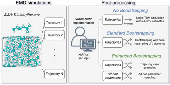
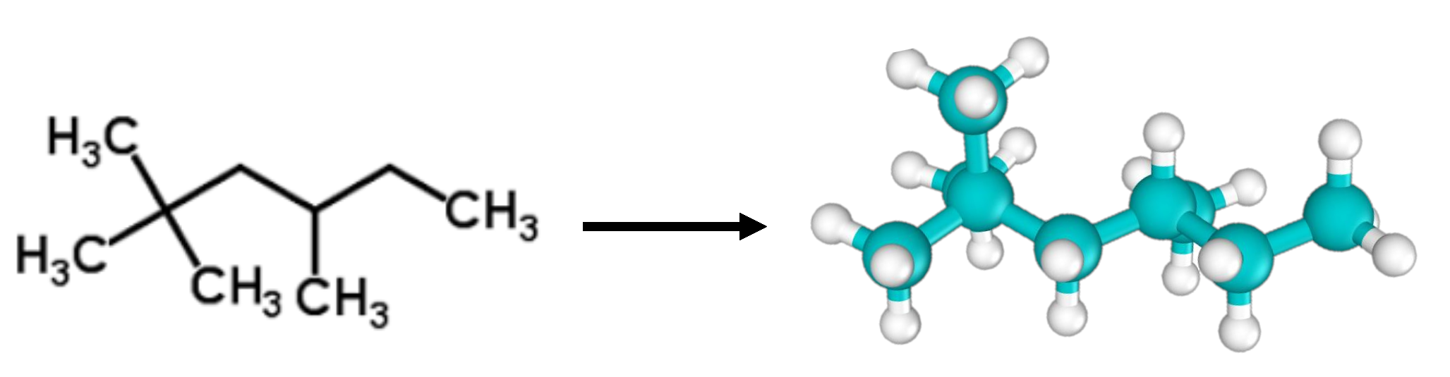
  • To demonstrate some case studies from equilibrium MD simulations of the lubricant 2,2,4-trimethylhexane performed at different temperatures and pressures.
  • To emphasize the importance of the meticulous post-simulation data analysis.
  • To show how ad hoc parameters can influence the viscosity.
The remainder of the paper is organized as follows: the details of the EMD simulation protocols, including the force field used, are given in Section 2.1. The technical details of the implementation of the TDM and the ad hoc parameters that can affect the simulation outcomes are highlighted in Section 2.2. The uncertainty quantification is described in Section 2.3. Section 3 presents results obtained with several different parameter choices in the implementation of the TDM under wide pressure and temperature ranges, representative for (T)EHL. Finally, conclusions are drawn in the last section.

2. Materials and Methods

2.1. EMD Protocol

EMD simulations were performed for the candidate molecule of the 10th IFPSC, 2,2,4-trimethlyhexane, C 9 H 20 (Figure 1), as the pressure-viscosity data already exist to validate the results in this work [42].
The COMPASS class II force field [37,44] was used to describe the interactions of the system. In this force field, anharmonic functions describe bonded interactions, and Van der Waals interactions are described by the 9-6 Lennard–Jones form to soften the repulsive part compared to the conventional 12-6 Lennard–Jones model. The general form of the potential energy for these force fields is given by:
E = E bond + E angle + E dihedral + E improper + E vdw + E electrostatic
where E bond , E angle , E dihedral , and E improper describe the bonded interactions in the system; and E vdw and E electrostatics describe the non-bonded Van der Waals and Coulombic interactions, respectively. Most EMD simulations were performed using a cubic simulation cell containing 100 molecules. The only exception was the initial validation, with a 1000-molecule cell, based on the repeated claim that finite-size effects on the shear viscosity are negligible [15,26,45,46,47]. The simulation cell was initialized with random positions and orientations of 2,2,4-trimethylhexane using Packmol [48]. To generate the necessary settings and parameters for the COMPASS force field, the msi2lmp tool was combined with the IOData Python library developed by Verstraelen et al. [49] to generate the correct file formats. The EMD simulations were performed with LAMMPS open-source MD simulation software [50]. The equations of motion for the atoms were integrated using the velocity Verlet algorithm [51] with a time step of 0.5 femtoseconds. The non-bonded Van der Waals interaction cut-off was set to 12 Å, and the sixth-power mixing rule was used for unlike-pair parameters. The pppm (particle–particle particle–mesh) method [52] is used to evaluate long-range electrostatic interactions with a desired relative error of 10 5 on the forces.
Equilibration and production MD runs were performed as follows: first, the energy of the cell was minimized with the conjugate gradient algorithm. After that, an NVT MD run was performed for 2 ns, followed by an NpT run for 4 ns at the desired pressures and temperatures using a Nosé–Hoover thermostat and barostat [53,54] with damping factors of 0.5 and 5.0 ps, respectively. The equilibrium density was extracted at the end of the NpT run using the pymbar.timeseries module [55], which automatically identifies and discards the equilibration or so-called "burn-in" region from the time-series data. Then, the atomic positions and box size of the last snapshot of the NpT run were slightly rescaled to match this equilibrium density, and production runs were performed in the canonical (NVT) ensemble. At this stage, 50 independent replicate NVT runs, which started from the same equilibrium configuration but with a different random seed for velocity assignment, were performed to improve statistics. The simulation time depends on the operating conditions and is mentioned in the Results section. The original TDM paper and several other studies reported that about 30 to 40 trajectories are sufficient to determine the shear viscosity (deviation less than 1%) [21,26]. Hence, the 50 independent trajectories used in this study were assumed to be sufficient.
Every picosecond, the time-integrated values of the stress tensor components were saved to a file using the fix ave/time LAMMPS command. This allowed us to reduce the storage requirements by at least three orders of magnitude, compared to simply writing out the stress tensor at each time step. While the implementation of the Green–Kubo integral in this work, Equation (2), is comparable to that of the OCTP LAMMPS plugin [47], all results required for post-processing are stored on a disk, allowing us to implement different post-processing strategies for the viscosity without repeating the EMD simulations.

2.2. The Determination of Shear Viscosity from EMD Simulations

This subsection presents the step-by-step implementation of the TDM and identifies ad hoc decisions within the protocol. As discussed in the introduction, the TDM starts by computing the running integral η n , α β ( Δ t ) in the Green–Kubo relation in Equation (2) for each trajectory n { 1 N } and each distinct pair of off-diagonal stress components, α and β . A double-exponential is fitted to the average over all η n , α β ( Δ t ) :
η ¯ ( Δ t ) = 1 3 N n = 1 N α β η n , α β ( Δ t ) η DE ( Δ t ) = C 1 ( 1 e Δ t / τ 1 ) + C 2 ( 1 e Δ t / τ 2 )
where the primed sum only considers the three upper (or lower) diagonal combinations of α and β . The final estimate of the viscosity is then
η = lim Δ t η DE ( Δ t ) = C 1 + C 2 .
The details of the non-linear regression, including the choice for the double-exponential form, are important because the estimated viscosity is sensitive to statistical fluctuations in η ¯ ( Δ t ) . The following paragraphs explain exactly how this fit is carried out in the TDM and other works. In addition, a new approach is introduced below to replace the manual steps in the TDM by a set of numerical algorithm to improve the overall reproducibility and to facilitate uncertainty quantification.
Before fitting the double-exponential, the standard deviation over the running integrals η n , α β ( Δ t ) is approximated by a simple power law:
σ ( Δ t ) = 1 3 N 1 n = 1 N α β η n , α β ( Δ t ) η ¯ ( Δ t ) 2 σ PL ( Δ t ) = a Δ t b ,
where a and b are the fitting parameters. The scaling Δ t b is used as a relative "measurement error" when fitting a model to η ¯ ( Δ t ) , or conversely, 1 / Δ t b is used as the weight in the regression. This ensures that better-resolved data points at smaller time lags have high weights in the fitting procedure than those at larger time lags. Previously, Rey-Castro and Vega [56] fitted the double exponential with a weight 1 / Δ t 2 . However, in the TDM, the weight was generalized to 1 / Δ t b with a fitted b, because a significant underestimation was observed for the viscosity of [BMIM][Tf2N] when using 1 / Δ t 2 . It should be noted that some studies applied different values for b without further justification [34,40]. For example, Kondratyuk and Pisarev [34] used b = 1 2 for all pressures ranging from 0.1 to 1000 M Pa . One might justify this choice by assuming that, at large time lags, the statistical estimate of η ¯ ( Δ t ) looks like a Brownian walk and is the time integral of an auto-correlation function consisting of uncorrelated sampling noise with a constant standard deviation [57]. These assumptions do not always hold: the auto-correlation function may have weak time correlations in its tail, and the magnitude of its statistical uncertainty increases as time lag increases.
Another important choice in the fit of the double-exponential is the set of time lags used to provide data for the fit. This is usually done by specifying a window of admissible Δ t values with an upper and lower bound. Zhang et al. introduced an empirical rule to set the upper bound for the fit, Δ t cut , to the time when σ ( Δ t ) reaches 40% of a user-defined guess of lim Δ t η ¯ ( Δ t ) [26]. The guess, η guess , is assumed to be visually identified as a plateau in a plot of η ¯ ( Δ t ) . For liquids with lower viscosity, e.g., at moderate pressure and high temperatures, it was claimed that 30% instead of 40% would change the calculated viscosity by only 1%. Still, the  40%-rule was proposed as a conservative and robust choice. The lower bound of the Δ t -window was chosen to exclude transient behavior η ¯ ( Δ t ) at time lags smaller than a few picoseconds. [15,26] Later works pointed out that the 40% rule has limited transferability. For example, Messerly et al. upgraded it to 80% to deal with the inherently slower dynamics when the viscosity increases [15,35].
The calculation of the viscosity in this work follows the TDM, as outlined in the following steps. Compared to the original protocol, each ad hoc parameter is described in more detail. Since these ad hoc decisions cannot be made rigorously, an interval of plausible ad hoc parameters is given whenever possible.
  • In principle, the first decisions in the TDM are the simulation time and the number of independent MD production runs, which are difficult to determine a priori. The production runs should be sufficiently longer than the inherent correlation times in the stress tensor fluctuations, which can only be determined after the simulation. If the results are not statistically converged with a given simulation length, one should extend the trajectories or generate more until the results are satisfactory (or all resources are exhausted).
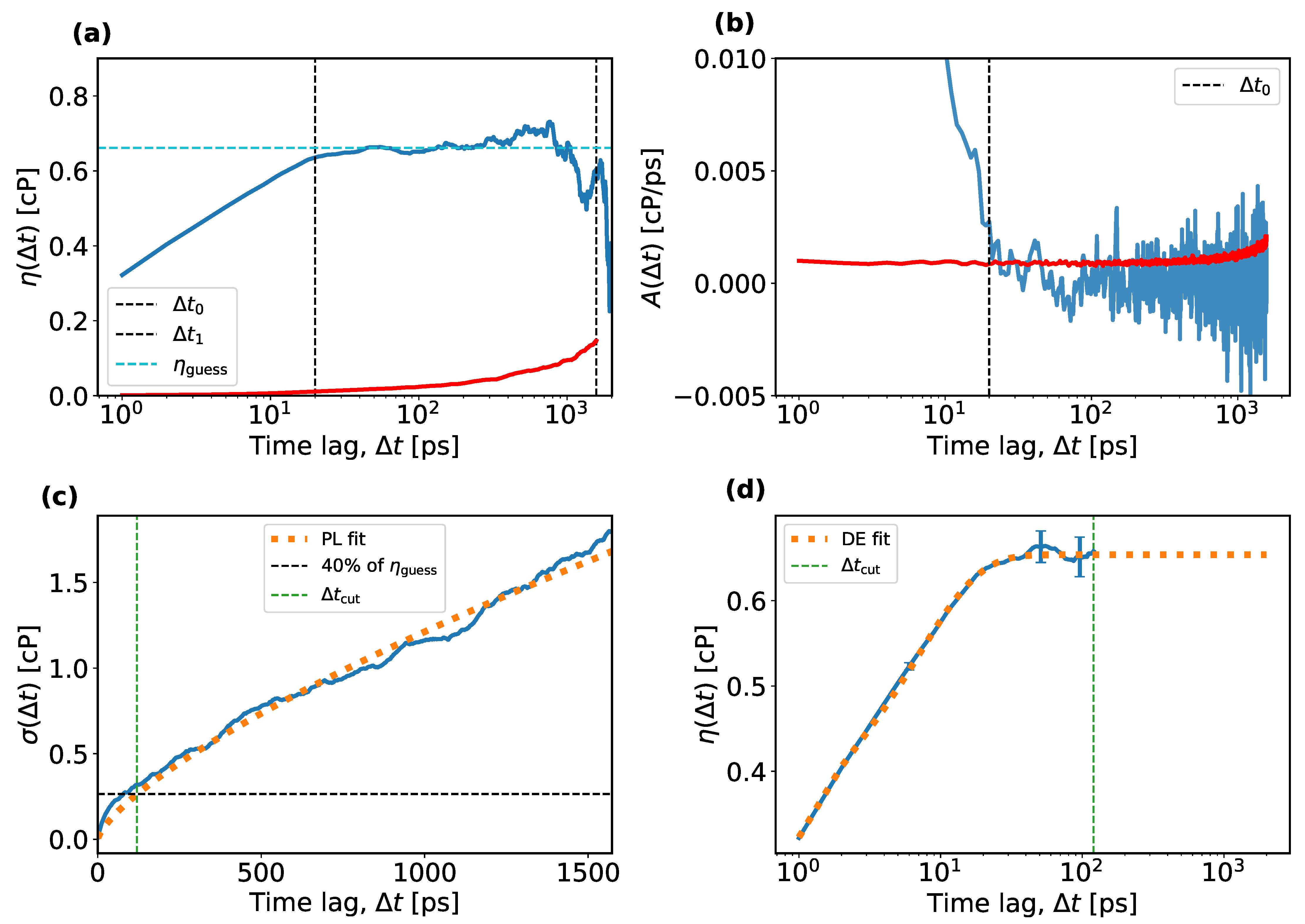
  • The average running integral, η ¯ ( Δ t ) ; the average autocorrelation function, A ¯ ( Δ t ) ; and the standard deviation, σ ( Δ t ) , are calculated over N independent EMD trajectories. Typical examples are shown as solid blue curves in Figure 2a–c, respectively. Figure 2a,b also contain the standard error on the plotted average as a function of Δ t , plotted as solid red curves.
  • For the TDM, one must identify a plateau-like region in η ¯ ( Δ t ) and determine a reasonable guess of the viscosity in that region. Practical instructions for making this guess were not described explicitly in previous works, so it is assumed here that this guess was made by a visual inspection of a plot such as the one shown in Figure 2a. However, when making such a plot, one must decide on the range of the time lags on the horizontal axis, which entails more empirical choices. Here, an algorithmic approach is introduced to guess the viscosity, which mimics the manual guess of the TDM as closely as possible. The algorithm first selects an upper and a lower bound for the time lags to identify the plateau region and then estimates the viscosity within that region. To set an upper bound of the plateau region, the standard error of the mean is compared to the average running integral and plotted in red and blue in Figure 2a, respectively. At overly large time lags, this error increases and makes it impossible to identify any plateau. Therefore, the upper bound for the time lag, Δ t 1 , is fixed in this work as the first point at which the standard error on the mean becomes significant compared to the average running integral, i.e.,  σ ( Δ t ) / 3 N > f 1 η ¯ ( Δ t ) , for which f 1 = 25 % is chosen. Other choices for f 1 could be considered, which is relevant for the uncertainty analysis explained later. It could be argued that any f 1 [ 10 % , 100 % ] could be used instead. (The uncertainty analysis reveals that the predicted viscosity is nearly insensitive to f 1 .) The lower bound, Δ t 0 , is set as the first time lag when the average auto-correlation function approaches zero by less than f 2 = 2 times the standard deviation of the mean over all auto-correlation functions. Both functions are shown in Figure 2b in blue and red, respectively. This corresponds to the onset of the tail of the auto-correlation function, A ¯ ( Δ t ) , after which the running integral, η ¯ ( Δ t ) , starts to level off and exhibit a plateau. Other values of f 2 could be considered, e.g., from the interval [ 1 , 3 ] . Higher values of f 2 are not recommended because these would force Δ t 0 into the interval where the auto-correlation function has not decayed to zero yet. Lower values of f 2 make Δ t 0 more susceptible to noise in the auto-correlation function. Instead of visually estimating the viscosity in the interval [ Δ t 0 , Δ t 1 ] , the q = 50 % quantile (the median) of all η ¯ ( Δ t ) values in this region is used as a guess of the viscosity, η guess . Other values in the interquartile range (IQR, q [ 25 % , 75 % ] ) could also be considered. The use of quantiles makes η guess insensitive to outliers in the plateau region.
  • The next step in the TDM is to fit the power law from Equation (6). One might expect the interval of the plateau region, [ Δ t 0 , Δ t 1 ] , be suitable for estimating a and b. In some cases, however, this leads to strong parameter correlations between a and b. Instead, σ ( Δ t ) is fitted in the interval [ 0 , Δ t 1 ] , which makes b less sensitive to statistical uncertainties. The time interval was not mentioned in the original TDM paper and may be specific to this work.
  • The parameter Δ t cut is then fixed as the time when the power-law fit reaches f 3 = 40 of η guess , which is illustrated by the dashed lines in Figure 2c. Other values for the percentage f 3 have been considered in the literature, ranging from to 20% to 80% [15,35,58].
  • Finally, the double-exponential model from Equation (4) is fitted with the curve_fit function from SciPy [59], to  η ¯ ( Δ t ) in the interval [ 0 , Δ t cut ] with a weight of 1 / Δ t b , where b is taken from the power-law fit. The final viscosity is the long-term limit of the double exponential fit. See the dotted orange curve in Figure 2d. Note that other works exclude small Δ t values from the fit because the double-exponential model is not suitable for small time lags. Since the time integral of the stress tensor is stored only every picosecond, transient effects at small time lags are de facto excluded from the fits.
    A nonlinear regression may have multiple solutions, i.e., local minima of the least-squares cost function. To help the optimization algorithm, an initial guess can be specified, for which C 1 = C 2 = η guess / 2 , τ 1 = Δ t cut / 3 and τ 2 = 2 Δ t cut / 3 have been used. By making the τ values different, the symmetry of the model is effectively broken and this makes the optimizer less likely to get stuck at a saddle point. To further facilitate the regression, the parameters τ 1 and τ 2 are bounded to the interval [ 0 , 3 Δ t cut ] . If one of the optimal τ i parameters reaches its upper bound and the corresponding C i is non-zero, the solution is marked as invalid and is excluded from the remaining analysis.
The TDM was applied in this work using the recommended values of the ad hoc choices at every step, except that subjective human decisions have been made explicit to the reader and are replaced by predefined rules to automate human decision making and assess its variability. Inevitably, to mimic human decision making, more ad hoc parameters were used than in the original TDM, namely, f 1 , f 2 , and q.
Every ad hoc decision has an impact on the outcome, which contributes to the uncertainty of the prediction. This uncertainty is estimated with Monte Carlo error propagation, as explained in the following subsection. Note that the Monte Carlo approach can only assess the impact of changes in numerical ad hoc parameters, though there are other ad hoc decisions, such as the power law and the double-exponential models, which also affect the final outcome.

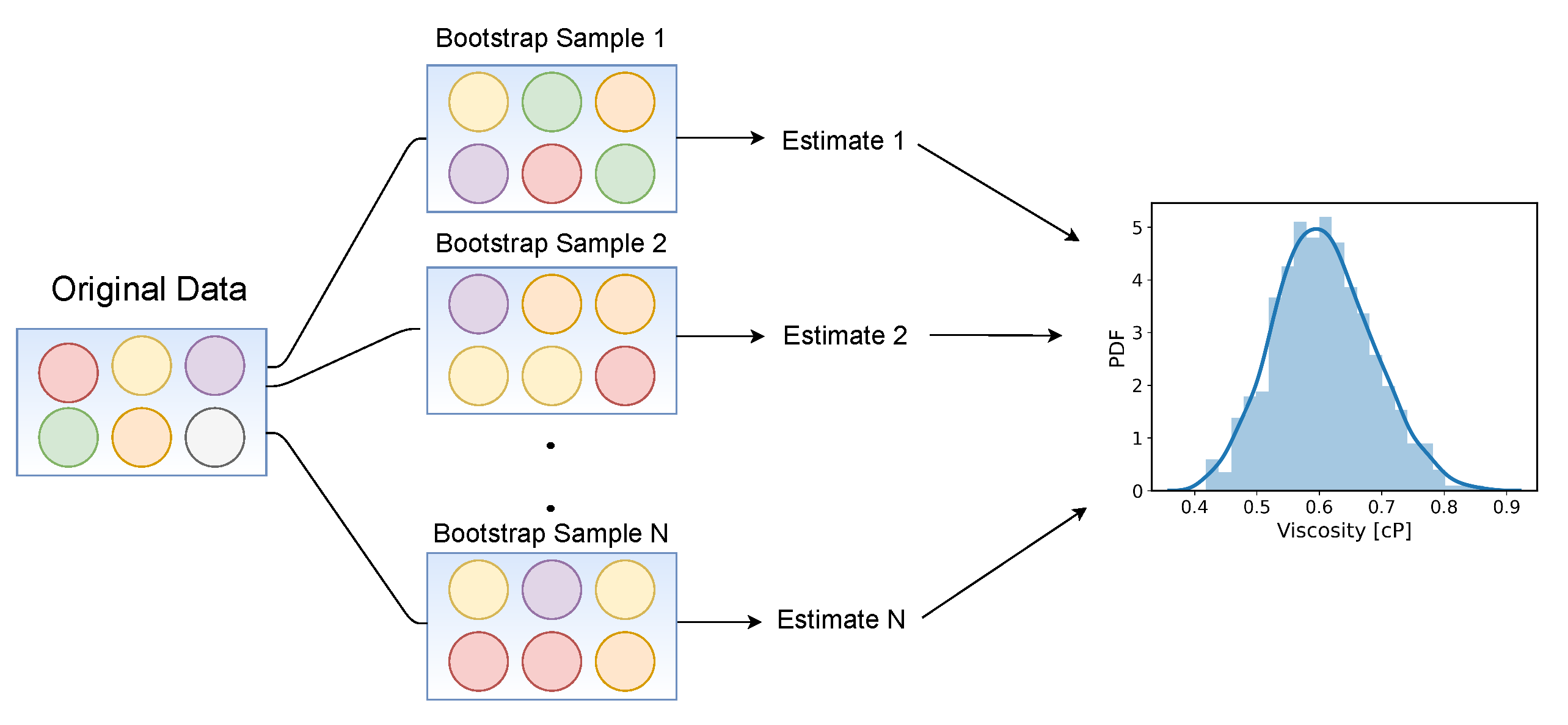
2.3. Uncertainty Quantification

In general, there are numerous sources of uncertainty in the MD simulations. These sources can be divided into two main categories: (1) systematic errors and (2) statistical errors. The first category involves the errors arising from, e.g., the inaccuracies in the chosen force fields, the finite-size effects, or the technical choices when performing MD simulations (e.g., convergence settings for the reciprocal Ewald sum). Errors in the second category are due to the thermal fluctuations in the MD simulations. All properties extracted from an MD trajectory are in fact sampling estimates of those properties and have some uncertainty due to the finite number of samples. When overly large statistical uncertainties are observed and computational resources are available, one may extend the trajectories or carry out more independent MD runs. The Green–Kubo approach derives the viscosity from the time-correlation functions of the stress tensor components, and such calculations are highly susceptible to statistical errors and require proper uncertainty quantification.
Monte Carlo error propagation is a general and broadly applicable technique for quantifying the uncertainty of a computational prediction due to uncertainties in the model’s inputs. The basic principle is to repeat the same simulation with different random input parameters, drawn from distributions that characterize their uncertainty. This results in a distribution of predications, which characterizes the uncertainty of the outcome.
One popular approach to generating random inputs for Monte Carlo error propagation is bootstrapping with case resampling. [15,35,60] It is applicable whenever a set of random quantities, instead of a single value, is used as input. Figure 3 illustrates the basic concept of the bootstrapping method. In this work, the viscosity was derived from 50 EMD trajectories, denoted as “Original data” in Figure 3. In one standard bootstrapping iteration, a set of 50 trajectories was sampled from the original set, with replacement, and the viscosity was then derived from the sample. This was repeated N bootstrap times, each time resulting in one plausible estimate of the viscosity. This led to an ensemble of predicted viscosities from which a mean and standard deviation can be derived, the latter being the statistical uncertainty in the predicted viscosity. By increasing N bootstrap , the bootstrapping error on the estimated uncertainty can be made arbitrarily small.
The bootstrapping method is easily extended to account for other sources of uncertainty. As it is essentially a Monte Carlo error propagation, one can also randomly sample other inputs while resampling the set of trajectories. In this work, the ad hoc parameters in the post-processing steps ( f 1 , f 2 , f 3 , and q described in the previous section) were also sampled to account for their arbitrariness. Normally, such choices are fixed by expert judgment, and any error in judgment would result in a systematic error, which is hard to assess for a single choice. In this work, ad hoc choices were randomly or algorithmically made, within the bounds of good practices from the literature, and the impacts of these choices on the simulation outcomes were analyzed.
In summary, the post-processing of the MD simulations was carried out in three different ways. The first approach was not to carry out any bootstrapping or parameter sampling (NB), and to compute just a single viscosity with the default TDM settings. The second strategy was to apply bootstrapping only to the set of trajectories but to keep the ad hoc parameters still fixed at their recommended values, as performed in a few studies in the literature [15,35,58], to estimate the error in viscosity, which will be referred to as “Standard Bootstrapping” (SB). Finally, the third approach also accounts for uncertainties due to ad hoc parameters by randomly sampling them in the ranges of plausible values mentioned in the previous section to mimic the arbitrariness of human decision making, which will be called “Enhanced Bootstrapping” (EB). For the case of simulations at ambient conditions, the Monte Carlo method was also used to elucidate which ad hoc parameters linearly correlate with the predicted viscosity. For clarity, Table 1 lists all settings and how these settings differed in each of the three approaches.

3. Results and Discussion

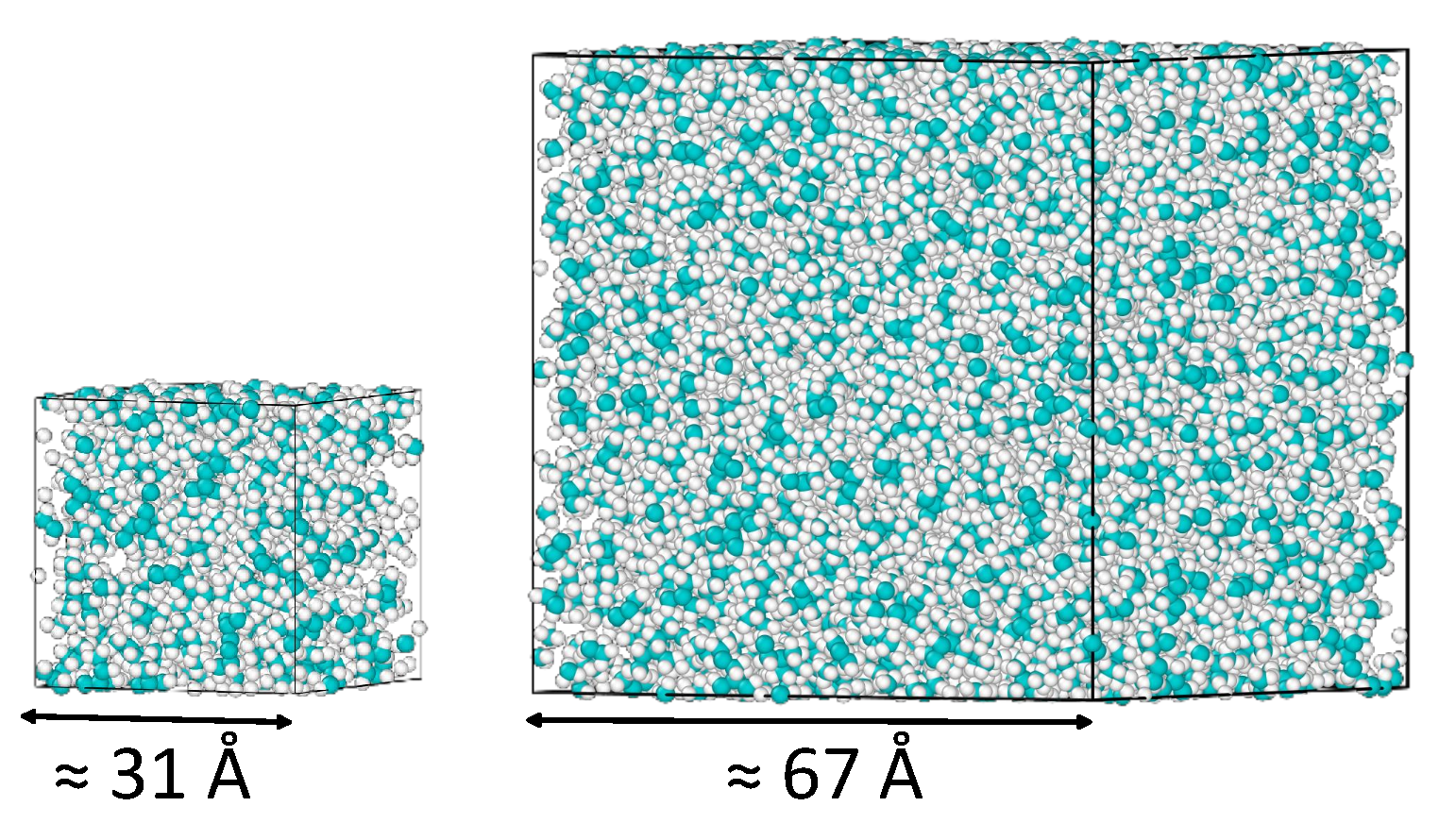
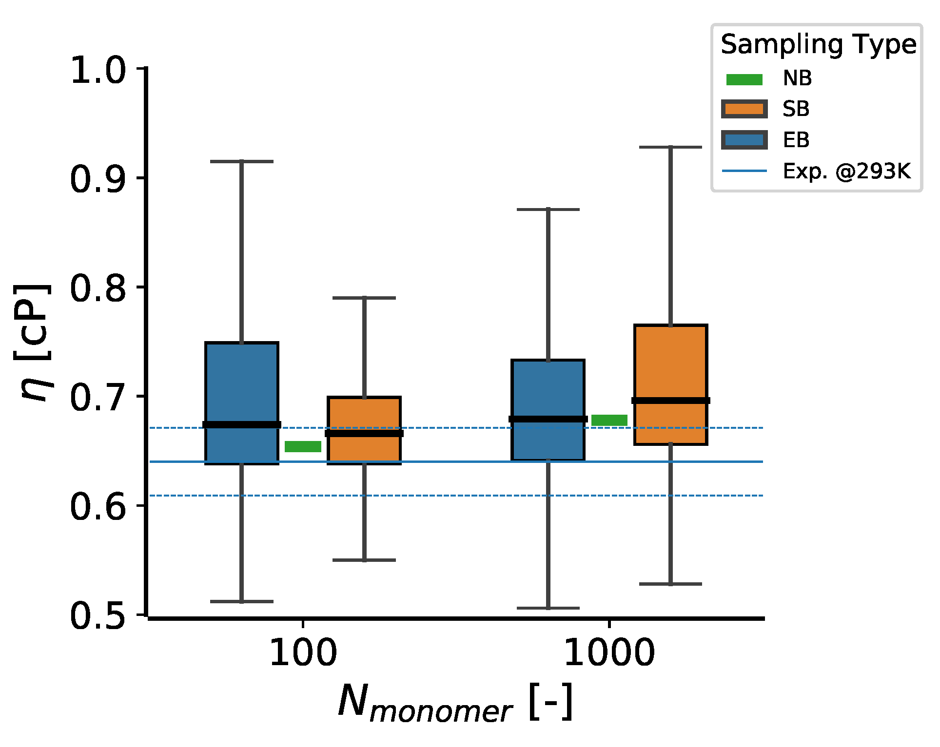
3.1. The Determination of the Viscosity of 2,2,4-Trimethylhexane at Ambient Conditions System Size Effects

While the finite-size effect on viscosity is well understood [61], it is often found to be negligible [15,26,45,46,47]. First, two systems containing 100 and 1000 molecules of 2,2,4-trimethylhexane, shown in Figure 4, were studied to check for possible systematic errors due to finite-size effects. For each system size, 50 NVT trajectories, each 2 ns long, were used.
The results, including equilibrium system density and box length, for both system sizes, are given in Table 2, for the three levels of post-processing, namely, NB, SB, and EB. In the cases of SB and EB, 5000 bootstrap samples were used to obtain the viscosity distributions, of which at most 2% of the double-exponential fits were marked invalid. The viscosity and its error are expressed using the median and median absolute deviation (MAD) metrics, as such metrics are robust to outliers. In both cases, the distributions obtained are right-skewed, with skewness values greater than zero. Other relevant parameters such as mean, mean absolute deviation, interquartile ranges, and histograms are presented in Table S1 and Figure S1 of the Supporting Material.
Figure 5 shows the variation in viscosity as a function of the number of molecules for each of the three levels of post-processing. As expected, a broader distribution of viscosity was obtained for the smaller system using enhanced bootstrapping due to the effect of changes in the ad hoc parameters combined with the effect of larger equilibrium fluctuations of the system. While the finite size effect seems to be more pronounced without bootstrapping (NB) and with standard bootstrapping (≈4%), it diminishes in the case of enhanced bootstrapping, meaning that the size dependence may be due to the ad hoc parameters. Any extrapolation towards an infinite box size would be premature at this stage because sampling uncertainties exceed the apparent size dependence. One would have to perform more simulations, also for more system sizes, and make the post-processing more robust, to reduce the uncertainties prior to the extrapolation. Since the main objective of this study was to show the influence of ad hoc choices in the TDM, further assessment of the size dependence was deferred to a later study, and the smaller system was used for the remainder of the analysis.

3.2. Dependence of the Viscosity on Ad Hoc Parameters

The enhanced bootstrapping procedure was used to reveal correlations between the predicted viscosity and the ad hoc parameters. Figure 6 depicts scatter plots of the viscosity as a function of f 1 , f 2 , q and f 3 . While the factor f 3 , which determines Δ t cut , showed a stronger linear correlation of around 22% (Pearson correlation coefficient), the effects of the other parameters are far less pronounced. In other words, the enhanced bootstrapping method showed that the 40% cut-off criterion introduced by the TDM does have a pronounced effect on the predicted viscosity, contrary to the findings of [58], who used (standard) bootstrapping with 200 iterations for 20 trajectories. Only for a subset of the bootstrap iterations, the dependence of η on f 3 was pronounced, which might explain why this correlation was overlooked in earlier works. Finally, it is encouraging that the ad hoc parameters introduced in this work ( f 1 , f 2 and q) correlate at worst weakly with the predicted viscosity.

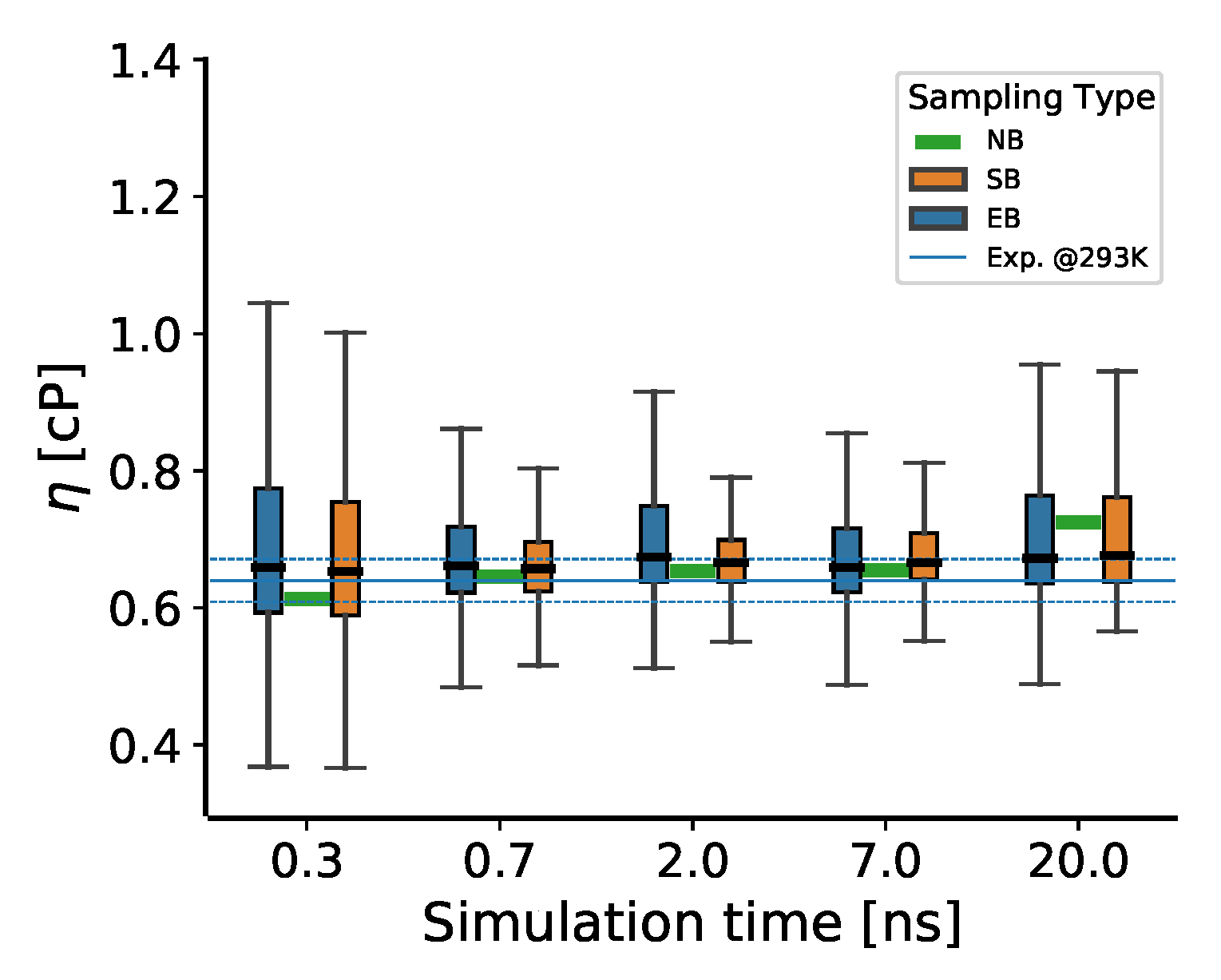
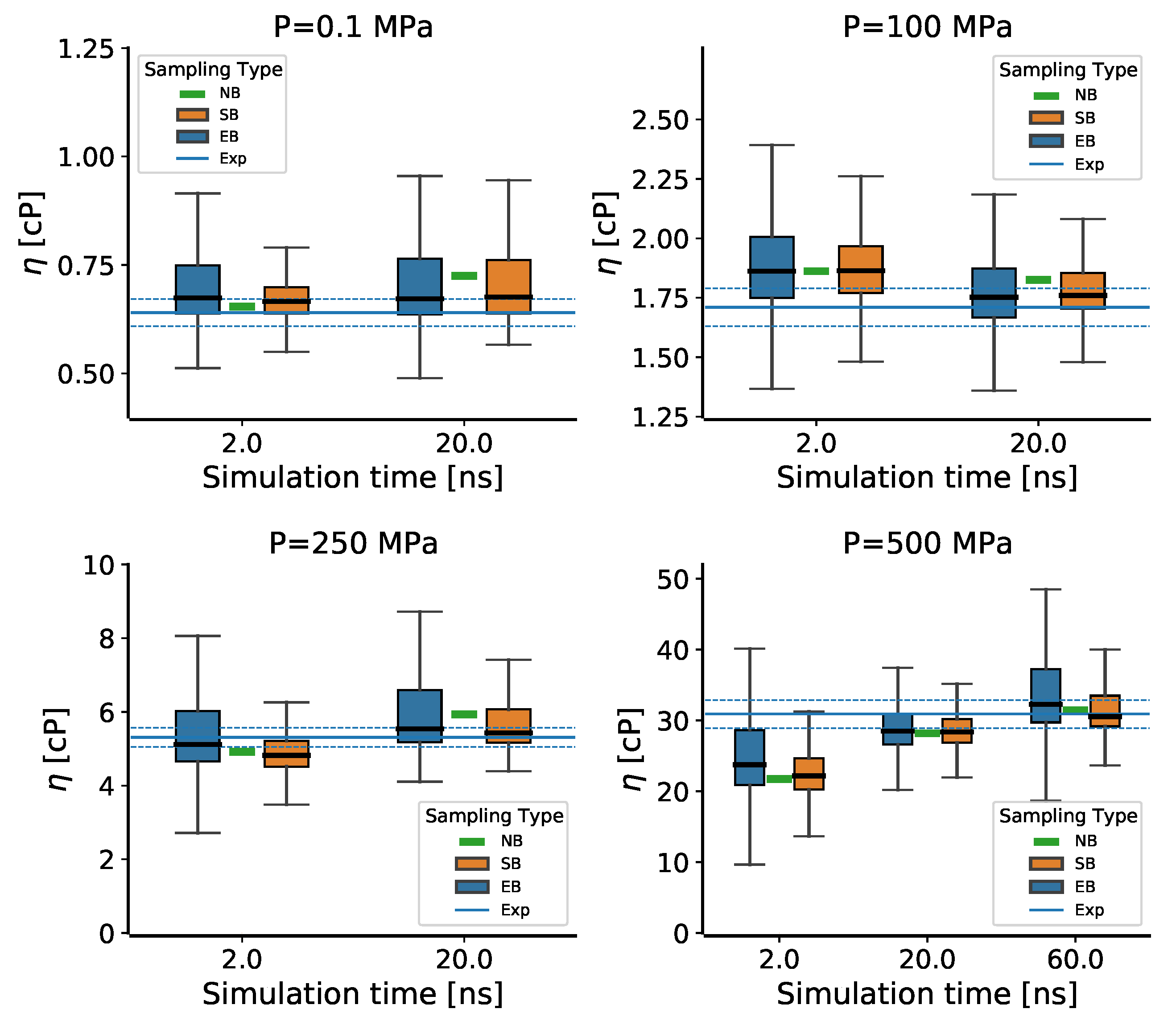
3.3. Simulation Length

The simulation length of each trajectory is important for the correct prediction of the viscosity. To limit the computational burden, one would like to reduce the simulation time of the individual trajectories to a minimum. However, if the simulation time is significantly shorter than the correlation time of the stress tensor fluctuations, it is challenging to integrate the auto-correlation function correctly, irrespective of the number of trajectories. As the adequate simulation time was unclear a priori, short simulations were performed first, and then the trajectory lengths were extended gradually from 300 ps to 20 ns. Fifty trajectories are used throughout, and the viscosity was calculated using the three levels of post-processing, again using 5000 iterations for the standard and enhanced bootstrapping.
Figure 7 shows the viscosity distributions obtained with different sampling types. As expected, broader viscosity distributions were obtained for the shortest simulation time with both standard and enhanced bootstrapping due to the limited time available for the system to equilibrate and the increased susceptibility to fluctuations. In general, enhanced bootstrapping estimates larger uncertainties, due to the sampling of TDM heuristics, in line with the results shown above. The deviation in the median viscosity became relatively small from 2 ns. This analysis shows again the importance of bootstrapping: without it (NB), one may incorrectly conclude that even 20 ns simulations are insufficient to converge the viscosity.
It can be concluded that it is reasonable to use 2 ns long single trajectories to obtain reliable estimates at ambient conditions for the molecule examined in this study. However, this assumption cannot be blindly generalized to other systems or operating conditions. Especially when the viscosity (and thus correlation times) increases, the required simulation time must be reassessed with a series of progressively longer simulations.

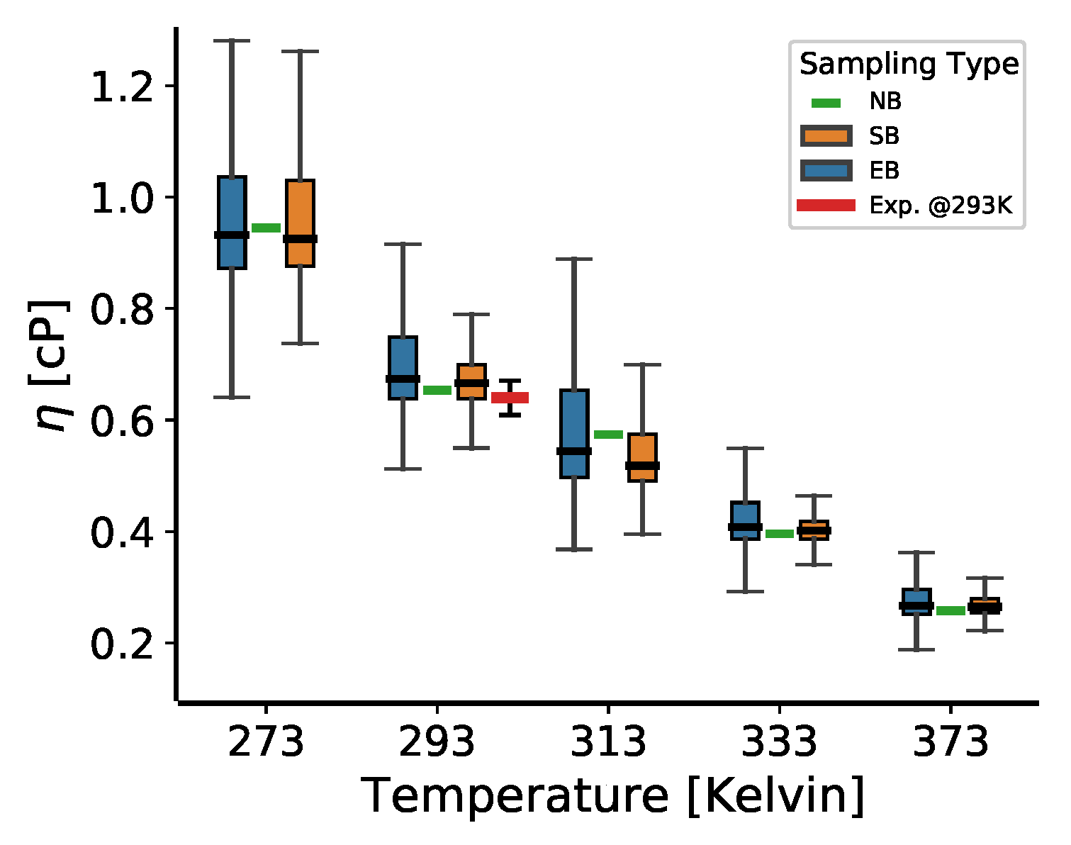
3.4. The Temperature Dependence of the Viscosity for 2,2,4-Trimethylhexane

To investigate the effect of temperature on viscosity, EMD simulations were performed this time for temperatures from 273 K to 373 K , again using 50 trajectories, each 2 ns long. The results are presented in Table S1 of the Supplementary Material. Furthermore, Figure 8 shows the effect of temperature on the viscosities calculated with the three post-processing scenarios. At higher temperatures, as a result of the decreased viscosity, all three methods gave closer estimates, and the effect of ad hoc choices became less pronounced. Still, for each temperature, enhanced bootstrapping resulted in larger uncertainties.
As there is no experimental η ( T ) data available for this lubricant molecule, the obtained results are only compared with the experimental data at 293 K .

3.5. The Pressure Dependence of the Viscosity for 2,2,4-Trimethylhexane

Lastly, the pressure dependence of the viscosity was investigated. EMD simulations were performed at higher pressures: 100, 250, and 500 MPa. Even though EMD was applied up to pressures of 1 G Pa in several other studies [34,35,62], it is computationally very challenging to obtain converged results with the TDM, as will be explained below. It is well-known that, as the pressure increases, the correlation times also increase as a result of slower system dynamics. Therefore, the simulation times should also be substantially increased at higher pressures to account for the increased viscosity.
Therefore, in this section, the results are compared once again with varying individual trajectory lengths. The analysis of the trajectory lengths in Section 3.1 showed that 2 ns long trajectories are sufficient to obtain reliable viscosity estimates at ambient conditions. This time, the aim was to investigate to which pressure this trajectory length would be sufficient for reliable estimates. Therefore, the viscosity was calculated for two different cases: 50 NVT trajectories (1) each 2 ns long and (2) each 20 ns long. For 500 MPa pressure, the viscosity showed a pronounced increase with simulation time, which motivated us to extend these trajectories to 60 ns.
Figure 9 shows the viscosities obtained with three different post-processing schemes introduced in this study at each pressure, with varying simulation times. For each case, enhanced bootstrapping resulted in wider distributions as a result of the underlying ad hoc parameter variations. The histograms of these distributions are shown in the Supplementary Material. In addition, the median viscosity, the error in viscosity calculated by the median absolute deviation, and other relevant statistical metrics for these distributions are presented in Table S1 of the Supplementary Material.
The Pearson correlation coefficient of η and f 3 was found to increase up to approximately 36% at 500 MPa when only 2.0 ns long individual trajectories were used with the enhanced resampling approach. The plots showing the correlation between the predicted viscosity and f 3 for three different simulation times at 500 MPa are given in Figure S8 of Supplementary Material. At all pressures studied, the longest EMD simulations in this work predicted viscosities in line with experimental reference data, which is encouraging, but still with relatively large uncertainties despite the extended simulation times.
The common practice in the literature of visualizing the running integral η ¯ ( Δ t ) with a logarithmic scale for the viscosity can give the false impression that it levels off in the limit of large time lags. For example, the TDM was applied with this type of plot, to pressures of up to 1 GPa for 2,2,4-trimethylhexane in one of the entries of the 10th IFPSC [34], using individual trajectories only a few ns long. To clarify the risks of inappropriate use of log scales, Figure 10 shows a plot of η ¯ ( Δ t ) from the simulations at 500 MPa for three different choices of the scales: linear-linear, linear-log, and log-linear. As seen in the figure, when η ¯ ( Δ t ) is plotted on a logarithmic scale, a flat region appears visually, which is simply the consequence of large values being compressed more up the logarithmic scale. In this respect, estimating η guess without looking at a plot is safer, as it does not depend on visualization details.

4. Conclusions

In this study, EMD simulations were performed with various operating conditions relevant to TEHL, followed by trajectory post-processing with the TDM. The post-processing of the raw EMD data were performed with three levels of uncertainty quantification: (i) a single TDM calculation without error estimates, (ii) bootstrapping with case resampling of trajectories only, and (iii) enhanced bootstrapping with trajectory case resampling and sampling of the ad hoc parameters. The enhanced bootstrapping is a new procedure introduced in this work to better understand the effects of the ad hoc parameters. The conclusions and findings of this study can be listed as follows:
  • An algorithmic alternative, introducing three new ad hoc parameters, was proposed to remove the subjective human guess of the viscosity from the TDM, for which three new ad hoc parameters had to be introduced. Through Monte Carlo error propagation with bootstrapping, it is shown that the new ad hoc parameters have no significant influence on the predicted viscosity.
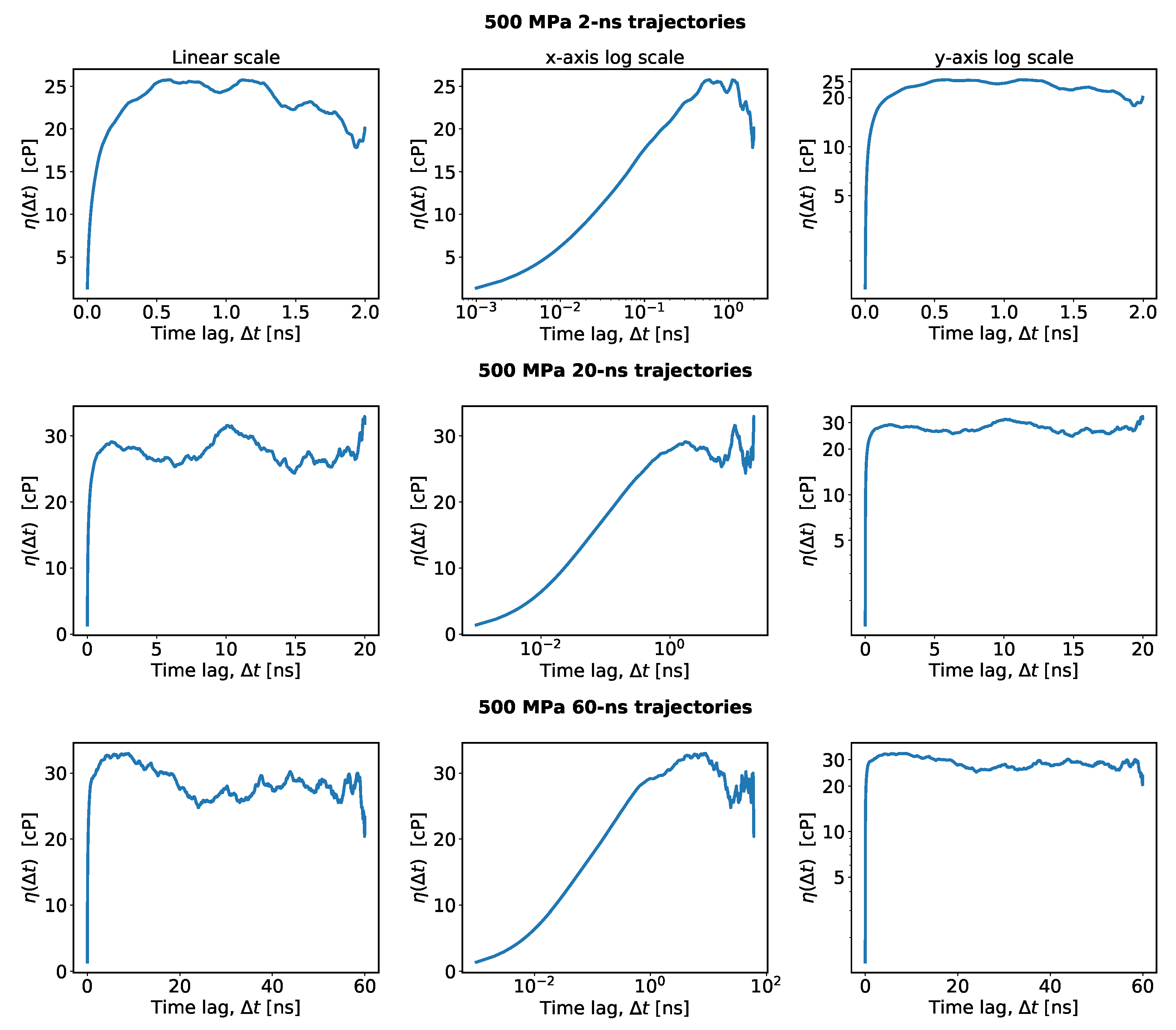
  • The proposed approach is not only convenient and robust, but it also eliminates the potentially obfuscating use of log scales, which can give the false impression that there is a stable plateau in η ¯ ( Δ t ) .
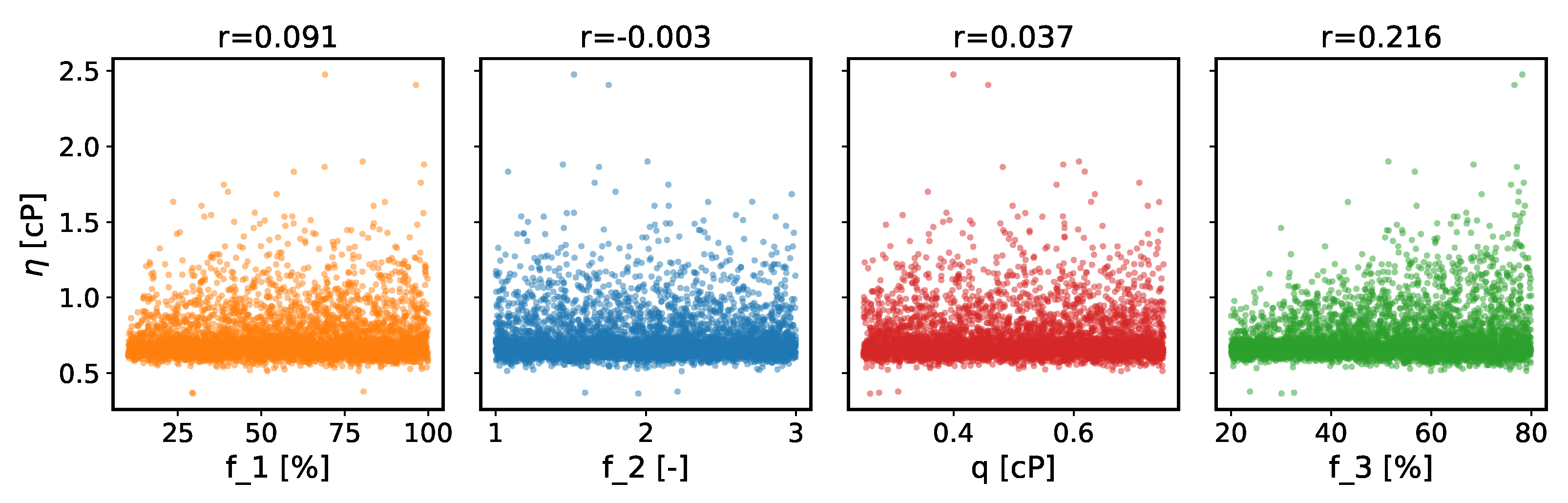
  • The viscosity predicted by the TDM depends on the ad hoc parameter f 3 , for which the original TDM paper recommends 40%. This is the percentage of the guessed viscosity used to estimate Δ t cut , up to which the double exponential is fitted. At ambient conditions, f 3 and the final η have a correlation coefficient of 22%, which rises to 36% at 500 MPa. By consequence, an (un)fortunate choice of this percentage can lead to an (un)favourable comparison to the experiment. This dependence was not noticed previously, presumably because these only considered scans of one ad hoc parameter at a time, whereas in this work the enhanced bootstrapping method varied all such parameters together.
  • The TDM, despite some of its limitations, still provides fairly good viscosity estimates in most cases, even without uncertainty quantification. However, when a systematic error is made due to an unfortunate choice of an ad hoc TDM parameter, only bootstrapping can clearly reveal this. Avoiding such errors becomes particularly challenging for lubricants under (T)EHL conditions, which are characterized by increased viscosity. To overcome this difficulty, it is suggested that the robustness of future improvements or alternatives to TDM should be thoroughly vetted with the enhanced bootstrapping method.
  • Clear communication and meticulous analysis of trajectories and uncertainties are essential for viscosity calculations using EMD simulations.
  • Future Scope
In future work, the presented analysis should also be applied to longer hydrocarbon molecules that are representative of lubricants. These are expected to have higher viscosity than the lubricant studied in this work (at the same temperature and pressure). Therefore, we also expect a higher sensitivity to the ad hoc parameters, which can be validated with the enhanced bootstrapping. Furthermore, the robustness and reliability of the MD post-processing could be further improved by eliminating the remaining ad hoc fitting models, such as the power law and the double exponential model.

Supplementary Materials

The following supporting information can be downloaded at: https://www.mdpi.com/article/10.3390/lubricants11040183/s1. Figure S1: Distributions obtained with (a,b) SB and (c,d) EB for 100- and 1000-monomer system sizes. While the η ¯ and σ how mean and the standard deviation, Md and MAD2 show the median and the median absolute deviation. Figure S2: Distributions obtained with SB for various simulation times for individual trajectories. Figure S3: Distributions obtained with EB for various simulation times for individual trajectories. Figure S4: Distributions obtained with SB at different temperatures. Figure S5: Distributions obtained with EB at different temperatures. Figure S6: Distributions obtained with SB for different pressures and simulation lengths. Figure S7: Distributions obtained with EB for different pressures and simulation lengths. Table S1: The relevant statistical metrics obtained using “Standard Bootstrapping” (SB) and “Enhanced Bootstrapping” (EB) with N bootstrap = 5000 for each case. The MAD1 values represent the mean absolute deviations, and the MAD2 values are the median absolute deviations. For the “No Bootstrapping” (NB) case, the single calculated viscosity is written in the median column. Figure S8: The correlation between the parameter f 3 and calculated viscosity with varying simulation times at 500 M Pa .

Author Contributions

Conceptualization, G.T., T.V. and D.F.; methodology, G.T. and T.V.; validation, G.T. and T.V.; formal analysis, G.T. and T.V.; investigation, G.T. and T.V.; resources, D.F.; data curation, G.T. and T.V.; writing—original draft preparation, G.T.; writing—review and editing, G.T., T.V. and D.F.; visualization, G.T.; supervision, T.V. and D.F.; project administration, T.V. and D.F.; funding acquisition, D.F. All authors have read and agreed to the published version of the manuscript.

Funding

This research was funded by Ghent University with grant number BOF.STA.2017.0030.01. The computational resources and services used were provided by Ghent University (Stevin and Hortense Supercomputer Infrastructures) and the VSC (Flemish Supercomputer Center), funded by the Research Foundation-Flanders (FWO).

Data Availability Statement

All the post-processing data used in this study are publicly available from Zenodo [63].

Conflicts of Interest

The authors declare no conflict of interest.

Abbreviations

The following abbreviations are used in this manuscript:
COMPASSCondensed-Phase Optimized Molecular Potentials for Atomistic Simulation Studies
DEDouble Exponential
EBEnhanced Bootstrapping
EMDEquilibrium Molecular Dynamics
GKGreen–Kubo
IFPSCInternational Fluid Properties Simulation Challange
LAMMPSLarge-scale Atomic/Molecular Massively Parallel Simulator
MADMedian Absolute Deviation
MiPPEMie Potentials for Phase Equilibria
NBNo Bootstrapping
NEMDNon-Equilibrium Molecular Dynamics
PLPower law
SBStandard Bootstrapping
TDMTime Decomposition Method
TEHLThermo-Elasto Hydrodynamic Lubrication

References

  1. Bair, S.; Martinie, L.; Vergne, P. Classical EHL Versus Quantitative EHL: A Perspective Part II—Super-Arrhenius Piezoviscosity, an Essential Component of Elastohydrodynamic Friction Missing from Classical EHL. Tribol. Lett. 2016, 63, 37. [Google Scholar] [CrossRef]
  2. Barus, C. Isothermals, isopiestics and isometrics relative to viscosity. Am. J. Sci. 1893, s3-45, 87–96. [Google Scholar] [CrossRef]
  3. Roelands, C.J.A.; Winer, W.O.; Wright, W.A. Correlational Aspects of the Viscosity-Temperature-Pressure Relationship of Lubricating Oils. J. Lubr. Technol. 1971, 93, 209–210. [Google Scholar] [CrossRef]
  4. McEwen, E. The Effect of Variation of Viscosity with Pressure on the Load-Carrying Capacity of the Oil Film between Gear-Teeth. J. Inst. Petroleum 1952, 38, 646–672. [Google Scholar] [CrossRef]
  5. Paluch, M.; Dendzik, Z.; Rzoska, S. Scaling of high-pressure viscosity data in low-molecular-weight glass-forming liquids. Phys. Rev. B Condens. Matter Mater. Phys. 1999, 60, 2979–2982. [Google Scholar] [CrossRef]
  6. Bair, S. Choosing pressure-viscosity relations. High Temp. High Press. 2015, 44, 415–428. [Google Scholar]
  7. Bair, S. Reference liquids for quantitative elastohydrodynamics: Selection and rheological characterization. Tribol. Lett. 2006, 22, 197–206. [Google Scholar] [CrossRef]
  8. Bair, S.; Yamaguchi, T.; Brouwer, L.; Schwarze, H.; Vergne, P.; Poll, G. Oscillatory and steady shear viscosity: The Cox–Merz rule, superposition, and application to EHL friction. Tribol. Int. 2014, 79, 126–131. [Google Scholar] [CrossRef]
  9. Bair, S. High Pressure Rheology for Quantitative Elastohydrodynamics; Elsevier: Amsterdam, The Netherlands, 2020. [Google Scholar] [CrossRef]
  10. Vergne, P.; Bair, S. Classical EHL versus quantitative EHL: A perspective Part i - Real viscosity-pressure dependence and the viscosity-pressure coefficient for predicting film thickness. Tribol. Lett. 2014, 54, 1–12. [Google Scholar] [CrossRef]
  11. Ewen, J.P.; Heyes, D.M.; Dini, D. Advances in nonequilibrium molecular dynamics simulations of lubricants and additives. Friction 2018, 6, 349–386. [Google Scholar] [CrossRef]
  12. Spikes, H.; Jie, Z. History, origins and prediction of elastohydrodynamic friction. Tribol. Lett. 2014, 56, 1–25. [Google Scholar] [CrossRef]
  13. Allen, M.P.; Tildesley, D.J. Computer Simulation of Liquids; Oxford University Press: Oxford, UK, 2017. [Google Scholar] [CrossRef]
  14. Chen, T.; Smit, B.; Bell, A.T. Are pressure fluctuation-based equilibrium methods really worse than nonequilibrium methods for calculating viscosities? J. Chem. Phys. 2009, 131, 2005–2007. [Google Scholar] [CrossRef] [PubMed]
  15. Messerly, R.A.; Anderson, M.C.; Razavi, S.M.; Elliott, J.R. Improvements and limitations of Mie λ-6 potential for prediction of saturated and compressed liquid viscosity. Fluid Ph. Equilibria 2019, 483, 101–115. [Google Scholar] [CrossRef]
  16. Carlson, D.J.; Giles, N.F.; Wilding, W.V.; Knotts, T.A. Liquid viscosity oriented parameterization of the Mie potential for reliable predictions of normal alkanes and alkylbenzenes. Fluid Ph. Equilibria 2022, 561, 113522. [Google Scholar] [CrossRef]
  17. Ewen, J.P.; Spikes, H.A.; Dini, D. Contributions of Molecular Dynamics Simulations to Elastohydrodynamic Lubrication. Tribol. Lett. 2021, 69, 24. [Google Scholar] [CrossRef]
  18. Behler, J. Perspective: Machine learning potentials for atomistic simulations. J. Chem. Phys. 2016, 145, 170901. [Google Scholar] [CrossRef]
  19. Devereux, C.; Smith, J.S.; Huddleston, K.K.; Barros, K.; Zubatyuk, R.; Isayev, O.; Roitberg, A.E. Extending the Applicability of the ANI Deep Learning Molecular Potential to Sulfur and Halogens. J. Chem. Theory Comput. 2020, 16, 4192–4202. [Google Scholar] [CrossRef]
  20. Batzner, S.; Musaelian, A.; Sun, L.; Geiger, M.; Mailoa, J.P.; Kornbluth, M.; Molinari, N.; Smidt, T.E.; Kozinsky, B. E(3)-equivariant graph neural networks for data-efficient and accurate interatomic potentials. Nat. Commun. 2022, 13, 2453. [Google Scholar] [CrossRef] [PubMed]
  21. Maginn, E.J.; Messerly, R.A.; Carlson, D.J.; Roe, D.R.; Elliott, J.R. Best Practices for Computing Transport Properties 1. Self-Diffusivity and Viscosity from Equilibrium Molecular Dynamics [Article v1.0]. Living J. Comput. Mol. Sci. 2019, 1, 6324. [Google Scholar] [CrossRef]
  22. Green, M.S. Markoff Random Processes and the Statistical Mechanics of Time-Dependent Phenomena. II. Irreversible Processes in Fluids. J. Chem. Phys. 1954, 22, 398–413. [Google Scholar] [CrossRef]
  23. Kubo, R. Statistical-Mechanical Theory of Irreversible Processes. I. General Theory and Simple Applications to Magnetic and Conduction Problems. J. Phys. Soc. Jpn. 1957, 12, 570–586. [Google Scholar] [CrossRef]
  24. Helfand, E. Transport Coefficients from Dissipation in a Canonical Ensemble. Phys. Rev. 1960, 119, 1–9. [Google Scholar] [CrossRef]
  25. Kajita, S.; Kinjo, T.; Nishi, T. Autonomous molecular design by Monte-Carlo tree search and rapid evaluations using molecular dynamics simulations. Commun. Phys. 2020, 3, 77. [Google Scholar] [CrossRef]
  26. Zhang, Y.; Otani, A.; Maginn, E.J. Reliable Viscosity Calculation from Equilibrium Molecular Dynamics Simulations: A Time Decomposition Method. J. Chem. Theory Comput. 2015, 11, 3537–3546. [Google Scholar] [CrossRef]
  27. Zhang, Y.; Guo, G.; Nie, G. A molecular dynamics study of bulk and shear viscosity of liquid iron using embedded-atom potential. Phys. Chem. Miner. 2000, 27, 164–169. [Google Scholar] [CrossRef]
  28. Alfè, D.; Gillan, M.J. First-principles calculation of transport coefficients. Phys. Rev. Lett. 1998, 81, 5161–5164. [Google Scholar] [CrossRef]
  29. Danel, J.F.; Kazandjian, L.; Zérah, G. Numerical convergence of the self-diffusion coefficient and viscosity obtained with Thomas–Fermi–Dirac molecular dynamics. Phys. Rev. Stat. Nonlinear Soft Matter Phys. 2012, 85, 066701. [Google Scholar] [CrossRef]
  30. Mondal, A.; Balasubramanian, S. A Molecular Dynamics Study of Collective Transport Properties of Imidazolium-Based Room-Temperature Ionic Liquids. J. Chem. Eng. Data 2014, 59, 3061–3068. [Google Scholar] [CrossRef]
  31. Kondratyuk, N.; Ryltsev, R.; Ankudinov, V.; Chtchelkatchev, N. Can We Accurately Calculate Viscosity in Multicomponent Metallic Melts? 2022. Available online: https://arxiv.org/abs/2211.03483 (accessed on 18 April 2023). [CrossRef]
  32. Balyakin, I.; Yuryev, A.; Filippov, V.; Gelchinski, B. Viscosity of liquid gallium: Neural network potential molecular dynamics and experimental study. Comput. Mater. Sci. 2022, 215, 111802. [Google Scholar] [CrossRef]
  33. Heyes, D.M.; Smith, E.R.; Dini, D. Shear stress relaxation and diffusion in simple liquids by molecular dynamics simulations: Analytic expressions and paths to viscosity. J. Chem. Phys. 2019, 150, 174504. [Google Scholar] [CrossRef]
  34. Kondratyuk, N.D.; Pisarev, V.V. Calculation of viscosities of branched alkanes from 0.1 to 1000 MPa by molecular dynamics methods using COMPASS force field. Fluid Ph. Equilibria 2019, 498, 151–159. [Google Scholar] [CrossRef]
  35. Messerly, R.A.; Anderson, M.C.; Razavi, S.M.; Elliott, J.R. Mie 16–6 force field predicts viscosity with faster-than-exponential pressure dependence for 2,2,4-trimethylhexane. Fluid Ph. Equilibria 2019, 495, 76–85. [Google Scholar] [CrossRef]
  36. Zheng, L.; Trusler, J.M.; Bresme, F.; Müller, E.A. Predicting the pressure dependence of the viscosity of 2,2,4-trimethylhexane using the SAFT coarse-grained force field. Fluid Ph. Equilibria 2019, 496, 1–6. [Google Scholar] [CrossRef]
  37. Sun, H. Compass: An ab initio force-field optimized for condensed-phase applications - Overview with details on alkane and benzene compounds. J. Phys. Chem. B 1998, 102, 7338–7364. [Google Scholar] [CrossRef]
  38. Potoff, J.J.; Bernard-Brunel, D.A. Mie Potentials for Phase Equilibria Calculations: Application to Alkanes and Perfluoroalkanes. J. Phys. Chem. B 2009, 113, 14725–14731. [Google Scholar] [CrossRef] [PubMed]
  39. Mick, J.R.; Soroush Barhaghi, M.; Jackman, B.; Schwiebert, L.; Potoff, J.J. Optimized Mie Potentials for Phase Equilibria: Application to Branched Alkanes. J. Chem. Eng. Data 2017, 62, 1806–1818. [Google Scholar] [CrossRef]
  40. Kondratyuk, N.D. Comparing different force fields by viscosity prediction for branched alkane at 0.1 and 400 MPa. J. Phys. Conf. Ser. 2019, 1385, 012048. [Google Scholar] [CrossRef]
  41. Kondratyuk, N.D.; Pisarev, V.V.; Ewen, J.P. Probing the high-pressure viscosity of hydrocarbon mixtures using molecular dynamics simulations. J. Chem. Phys. 2020, 153, 154502. [Google Scholar] [CrossRef]
  42. Bair, S. The pressure dependence of viscosity for 2,2,4 trimethylhexane to 1 GPa along the 20 C isotherm. Fluid Ph. Equilibria 2019, 488, 9–12. [Google Scholar] [CrossRef]
  43. Stukowski, A. Visualization and analysis of atomistic simulation data with OVITO-the Open Visualization Tool. Model. Simul. Mater. Sci. Eng. 2010, 18, 015012. [Google Scholar] [CrossRef]
  44. Sun, H.; Jin, Z.; Yang, C.; Akkermans, R.L.C.; Robertson, S.H.; Spenley, N.A.; Miller, S.; Todd, S.M. COMPASS II: Extended coverage for polymer and drug-like molecule databases. J. Mol. Model. 2016, 22, 47. [Google Scholar] [CrossRef] [PubMed]
  45. Moultos, O.A.; Zhang, Y.; Tsimpanogiannis, I.N.; Economou, I.G.; Maginn, E.J. System-size corrections for self-diffusion coefficients calculated from molecular dynamics simulations: The case of CO2, n-alkanes, and poly(ethylene glycol) dimethyl ethers. J. Chem. Phys. 2016, 145, 074109. [Google Scholar] [CrossRef] [PubMed]
  46. Daivis, P.J.; Evans, D.J. Transport coefficients of liquid butane near the boiling point by equilibrium molecular dynamics. J. Chem. Phys. 1995, 103, 4261–4265. [Google Scholar] [CrossRef]
  47. Jamali, S.H.; Wolff, L.; Becker, T.M.; De Groen, M.; Ramdin, M.; Hartkamp, R.; Bardow, A.; Vlugt, T.J.; Moultos, O.A. OCTP: A Tool for On-the-Fly Calculation of Transport Properties of Fluids with the Order- n Algorithm in LAMMPS. J. Chem. Inf. Model. 2019, 59, 1290–1294. [Google Scholar] [CrossRef]
  48. Allouche, A.R. Software News and Updates Gabedit—A Graphical User Interface for Computational Chemistry Softwares. J. Comput. Chem. 2012, 32, 174–182. [Google Scholar] [CrossRef]
  49. Verstraelen, T.; Adams, W.; Pujal, L.; Tehrani, A.; Kelly, B.D.; Macaya, L.; Meng, F.; Richer, M.; Hernández-Esparza, R.; Yang, X.D.; et al. IOData: A python library for reading, writing, and converting computational chemistry file formats and generating input files. J. Comput. Chem. 2021, 42, 458–464. [Google Scholar] [CrossRef]
  50. Thompson, A.P.; Aktulga, H.M.; Berger, R.; Bolintineanu, D.S.; Brown, W.M.; Crozier, P.S.; in’t Veld, P.J.; Kohlmeyer, A.; Moore, S.G.; Nguyen, T.D.; et al. LAMMPS - a flexible simulation tool for particle-based materials modeling at the atomic, meso, and continuum scales. Comput. Phys. Commun. 2022, 271, 108171. [Google Scholar] [CrossRef]
  51. Swope, W.C.; Andersen, H.C.; Berens, P.H.; Wilson, K.R. A computer simulation method for the calculation of equilibrium constants for the formation of physical clusters of molecules: Application to small water clusters. J. Chem. Phys. 1982, 76, 637–649. [Google Scholar] [CrossRef]
  52. Hockney, R.W.; Eastwood, J.W. Computer Simulation Using Particles; CRC Press: Boca Raton, FL, USA, 2021. [Google Scholar] [CrossRef]
  53. Nosé, S. A molecular dynamics method for simulations in the canonical ensemble. Mol. Phys. 1984, 52, 255–268. [Google Scholar] [CrossRef]
  54. Hoover, W.G. Canonical dynamics: Equilibrium phase-space distributions. Phys. Rev. A 1985, 31, 1695–1697. [Google Scholar] [CrossRef]
  55. Chodera, J.D. A Simple Method for Automated Equilibration Detection in Molecular Simulations. J. Chem. Theory Comput. 2016, 12, 1799–1805. [Google Scholar] [CrossRef] [PubMed]
  56. Rey-Castro, C.; Vega, L.F. Transport properties of the ionic liquid 1-ethyl-3-methylimidazolium chloride from equilibrium molecular dynamics simulation. the effect of temperature. J. Phys. Chem. B 2006, 110, 14426–14435. [Google Scholar] [CrossRef] [PubMed]
  57. Zwanzig, R.; Ailawadi, N.K. Statistical Error Due to Finite Time Averaging in Computer Experiments. Phys. Rev. 1969, 182, 280–283. [Google Scholar] [CrossRef]
  58. Schmitt, S.; Fleckenstein, F.; Hasse, H.; Stephan, S. Comparison of Force Fields for the Prediction of Thermophysical Properties of Long Linear and Branched Alkanes. J. Phys. Chem. B 2023, 127, 1789–1802. [Google Scholar] [CrossRef] [PubMed]
  59. Virtanen, P.; Gommers, R.; Oliphant, T.E.; Haberland, M.; Reddy, T.; Cournapeau, D.; Burovski, E.; Peterson, P.; Weckesser, W.; Bright, J.; et al. SciPy 1.0: Fundamental Algorithms for Scientific Computing in Python. Nat. Methods 2020, 17, 261–272. [Google Scholar] [CrossRef]
  60. Efron, B.; Tibshirani, R. An Introduction to the Bootstrap; Chapman and Hall/CRC: New York, NY, USA, 1994. [Google Scholar] [CrossRef]
  61. Kim, K.S.; Kim, C.; Karniadakis, G.E.; Lee, E.K.; Kozak, J.J. Density-Dependent finite system-size effects in equilibrium molecular dynamics estimation of shear viscosity: Hydrodynamic and configurational study. J. Chem. Phys. 2019, 151, 104101. [Google Scholar] [CrossRef]
  62. Mathas, D.; Holweger, W.; Wolf, M.; Bohnert, C.; Bakolas, V.; Procelewska, J.; Wang, L.; Bair, S.; Skylaris, C.K. Evaluation of Methods for Viscosity Simulations of Lubricants at Different Temperatures and Pressures: A Case Study on PAO-2. Tribol. Trans. 2021, 64, 1138–1148. [Google Scholar] [CrossRef]
  63. Toraman, G.; Verstraelen, T.; Fauconnier, D. EMD data for the paper “Impact of ad hoc post-processing parameters on the lubricant viscosity calculated with equilibrium molecular dynamics simulations” version 0.1.1, Zenodo (accessed on 13 April 2023). [CrossRef]
Figure 1. 2,2,4-Trimethylhexane and its representation in the EMD simulations. Cyan and white spheres represent carbon and hydrogen atoms, respectively. The molecular representation was drawn using the Ovito visualization tool [43].
Lubricants 11 00183 g001
Figure 2. The four panels depict (a) the average running integral, η ¯ ( Δ t ) ; (b) the average autocorrelation function, A ¯ ( Δ t ) ; (c) the standard deviation of the 3 N individual running integrals, σ ( Δ t ) , with the power-law (PL) fit; and (d) the truncated average running integral, η ¯ ( Δ t ) , with the double-exponential (DE) fit. Panels (a,b) also contain the standard deviations of the averages as red solid curves. Panels (c,d) show the fitted models as orange dotted curves. All panels contain dashed horizontal and vertical lines, corresponding to quantities Δ t 0 , Δ t 1 , η guess , and Δ t cut described in the text. The results are given for 100 molecules of 2,2,4-trimethylhexane at ambient conditions ( T   =   293   K , P   =   0.1   MPa ). Averages and uncertainties were computed over 50 trajectories of 2 ns long, each containing three off-diagonal components.
Lubricants 11 00183 g002
Figure 3. The schematic for the bootstrap resampling method for uncertainty quantification. The viscosity estimates have been obtained from each bootstrap sample, and a distribution was obtained using these estimates.
Lubricants 11 00183 g003
Figure 4. The simulation boxes containing 100 and 1000 2,2,4-trimethylhexane molecules. The carbon and hydrogens atoms are represented with cyan and white spheres, respectively—prepared using the Ovito visualization tool [43].
Lubricants 11 00183 g004
Figure 5. The variation in viscosity as a function of system size was computed with three levels of post-processing: “No Bootstrapping” (NB), “Standard Bootstrapping” (SB), and “Enhanced Bootstrapping” (EB) at 293 K, 0.1 MPa. The blue solid horizontal line shows the experimental viscosity at ambient conditions, and the dashed lines show its uncertainty.
Lubricants 11 00183 g005
Figure 6. Scatter plots showing the dependence of the viscosity on the introduced fudge factors, namely, f 1 , f 2 , q, and f 3 . The Pearson correlation coefficient is shown on top of each panel.
Lubricants 11 00183 g006
Figure 7. The variation in viscosity as a function of simulation time with three levels of post-processing under ambient conditions (293 K, 0.1 MPa).
Lubricants 11 00183 g007
Figure 8. The viscosity as a function of temperature with three levels of post-processing at 0.1 MPa. The red line shows the experimental viscosity at 293 K, including its uncertainty.
Lubricants 11 00183 g008
Figure 9. The variation in viscosity calculated using three levels of uncertainty analysis (none, standard, and enhanced bootstrapping) at 293 K and pressures of up to 500 MPa as a function of simulation time. The experimental viscosity values and the uncertainties at these pressures are shown with blue horizontal solid and dashed lines, respectively and can be found in Table 1 of reference [42].
Lubricants 11 00183 g009
Figure 10. Plots of η ¯ ( Δ t ) at 500 MPa for 2 ns long (upper panel), 20 ns long (middle), and 60 ns long (lower panel) individual trajectories. In the first column, the data are represented on a linear scale, whereas in the second and the third columns, the data are represented with logarithmic scales for the x- and y-axes, respectively.
Lubricants 11 00183 g010
Table 1. Overview of the three levels of EMD post-processing. “No Bootstrapping” (NB) refers to a single viscosity calculation without uncertainty quantification. “Standard Bootstrapping” (SB) applied bootstrapping to trajectories only. “Enhanced Bootstrapping” (EB) also included Monte Carlo error propagation of ad hoc parameters.
Bootstrapping Approach
ParameterNBSBEB
Resampling of trajectoriesNoYesYes
f 1 25%25%[10%, 100%]
f 2 22[1, 3]
q50%50%[25%, 75%]
f 3 40%40%[20%, 80%]
Table 2. System properties (i.e., number of molecules, cubic box length, and density) and viscosities obtained using the three different levels of post-processing analysis, namely, “No Bootstrapping” (NB), “Standard Bootstrapping” (SB), and “Enhanced Bootstrapping” (EB).
η [cP]
SystemBootstrapping Approach
N monomer L x [Å] ρ [ g   cm 3 ] NBSBEB
10030.90.721 ± 0.0090.6540.666 ± 0.0300.674 ± 0.045
100066.60.721 ± 0.0030.6780.696 ± 0.0470.679 ± 0.045
0.64 ± 0.031 1
1 Experimental [42].
Disclaimer/Publisher’s Note: The statements, opinions and data contained in all publications are solely those of the individual author(s) and contributor(s) and not of MDPI and/or the editor(s). MDPI and/or the editor(s) disclaim responsibility for any injury to people or property resulting from any ideas, methods, instructions or products referred to in the content.

