Abstract
BL Lac object 3C 371 is variable in optical and radio range, according to long-term monitoring data, for example AAVSO (American Association of Variable Star Observers) and OVRO (Owens Valley Radio Observatory). In addition, some authors note intra-night variability. However, in terms of access, just a few works are devoted to this topic, and questions remain about intra-day variability in radio range. The purpose of the work is to search for fast variability in radio (5, 6.1, 6.7 GHz) and optical bands (V, R, I) using international cooperation in 2019 and 2020 observation sessions. The 16-m radio telescope VIRAC, in Latvia, as well as optical telescopes AZT-3 (Mayaki, Ukraine), VNT (Vihorlat, Slovakia), and Schmidt camera (Baldone, Latvia) were used. To analyze variability, the STFT method of spectrograms and Lomb–Scargle periodograms for non-uniform time series were used. As result of the work, there is no correlation between optical and radio observations, and no significant quasi-harmonic variability was detected in radio range, but there is irregular low amplitude variability. In the optical range, there is variability with a characteristic time of about seven days and possibly less. Cyclical variability of 3C 371 was found in the optical range, and intra-day variability in radio range is most likely absent, as there are irregular variations and noise. It is planned to continue joint radio-optical observations 3C 371 to accumulate the necessary statistics.
1. Introduction
Herein, 3C 371 refers to BL Lacertae type objects (type of active galactic nucleus, named after its prototype, BL Lacertae) and is located in the Draco constellation of the northern sky, and is one of the closest and brightest objects of this type. Coordinates in the sky are: RA 18 h 6 min 50.681 s, Dec +69°49′28.11″, Redshift: 0.051, which is approximately 730 million light years from Earth. Apparent magnitude: 14.4 (V). Moreover, 3C 371 has not only a radio jet, but also an optical jet, discovered from observations at a ground telescope and confirmed by observations at the Hubble Space Telescope [1]. According to observations at the X-Ray orbiting telescope Chandra, an X-ray jet was also detected in 3C 371 [2]. It is assumed that the angle between the jet axis and the observer’s line of sight is less than 18° [1], but during a long-term (1994–2020) study the angular structure of 3C 371 in the radio range on the North American VLBA system, superluminal velocities of the bright components of the jet were not detected (http://www.physics.purdue.edu/astro/MOJAVE/sourcepages/1807+698.shtml), which is unusual for BL Lac objects. Old photographic plates with 3C 371 images, obtained since 1895, are well preserved, which made it possible to estimate the amplitude of optical variability of this object in the limit ±1.5 m [3].
Relatively high brightness in both the optical and radio ranges, as well as its convenient location (high declination), make 3C 371 an attractive object of study in many scientific groups. At the same time, there is a discrepancy in the nature of the intra-day variability of this object in the radio and optical ranges.
Thus, the presence of 3C 371 intra-day variability in the optical range has been confirmed by many observations since the 1960s. Also, the intra-day variability of this BL Lac object is confirmed in the gamma range [4]. At the same time, there is very little information about the presence or absence of intra-day and inter-day variability in the radio range, since such observations were mostly episodic and short-term. The purpose of this work was to obtain data for the study of rapid variations of 3C 371 flux density in the radio range. For a comparison with the data in the optical range, a program of quasi-simultaneous optical observations was organized at the observatories, located close to the meridian in Ventspils, but at different latitudes. This provided a more reliable acquisition of optical observation data, which depend on weather conditions.
This paper presents the results of the observation program (September–December 2019, July 2020) obtained in the radio range on the 16-m antenna of the Ventspils International Radio Astronomy Center (VIRAC, Latvia), at frequencies 5, 6.1, and 6.7 GHz, as well as optical observations, obtained at the observatories Mayaki (Ukraine), Vihorlat (Slovakia), and Baldone (Latvia) in optical bands V, R, and I, during Autumn–Winter 2019 and Spring–Summer 2020.
2. Materials and Methods
Radio observations were carried out on the 16-m diameter radio telescope with parabolic antenna, located in the Irbene village, Latvia. Operating frequencies of 5, 6.1, 6.7, and 8 GHz were used, however 8 GHz frequency was not used due to high interference in the observation time interval. Optical observations were obtained at the Mayaki Observatory (Odessa I.I. Mechnikov National University, Ukraine) using the AZT-3 telescope (V, R bands) with a mirror diameter of 48 cm; at the Vihorlat observatory (Slovakia) on the VNT telescope (V, R, I bands) with a mirror diameter of 1 m; at the Baldone observatory (Latvia) on a Schmidt camera (R band) with a mirror diameter of 1.2 m.
The 16-m radio telescope is equipped with a cryogenic (cooled with liquid helium) full power receiver (in two circular polarization, left (LCP) and right (RCP)), tuned to frequencies 5, 6.1, 6.7, and 8 GHz, with a back-end SDR-detector allowing for quick adjustment of the receiving parameters. To obtain points of the flux density, the technique of alternate pointing of the antenna beam at the target source, the calibration source, and the background sky field is used. The 3C 295 radio galaxy was used as a calibration source.
Brief technical parameters of the radio telescope are given in Table 1.

Table 1.
Technical information about the 16-m VIRAC radio telescope.
To obtain points of the flux density in the Janskys, the following technique is used. After pointing the telescope at the source and choosing the observation frequency, the source is measured (TPsrc1), then the background of the sky area (TPsky) is measured, followed by further measurement of background in the sky area with the included noise generator (calibrated noise diode) (TPcal) and control measurement of source (TPsrc2), to reduce the influence of external noise and change the angle of the telescope. The flux of the investigated radio source in Jansky:
where denotes receiver temperature increment per flux unit in (gain), the system temperature in K, the curve of gain versus antenna elevation angle, and the flux of calibration radio source. As a result, the measurement of the flux density in Jansky and its standard deviation is recorded to the data file. Obtaining one flux density measurement of radio source takes about 20 s. Seven consecutive measurements at the same frequency are averaged to reduce atmospheric and noise effects.
In 2017 and 2018, in order to study the manifestations of intra-day (IDV) radio variability of extragalactic objects, many test observations of variable and permanent (calibration) radio sources were carried out, the observation technique was debugged and the equipment was tuned in order to study fast radio variability of extragalactic objects. Operation of the radio telescope is fully automated. It is remotely controlled from the VIRAC office in Ventspils. More detailed information about the methodology for conducting observations and obtaining the flux density of radio sources in Janskys, as well as information about testing the radio telescope and studying its parameters, is presented in the work [5].
During the preliminary processing of radio observation data, polynomial smoothing was applied (for individual observation sessions) by the Savitsky–Golay method [6]. To construct the time-frequency spectrograms, a windowed Fourier transform was used [7]. Since the calculation of spectrograms requires a uniform time step between samples, the already smoothed radio data were interpolated with a B-spline [8] since it practically does not give false splashes and distortions at the break points of the data series.
To calculate periodograms and construct trigonometric polynomials, which were used in the analysis of optical observation data, the popular Lomb–Scargle method [9] was used for uneven time series of astronomical observations.
3. Results
3.1. Radio Observations
Observations of 3C 371 were carried out on 2–10 September 2019 at frequencies 5 and 6.1 GHz. Plots of this initial and smoothed data for left (LCP) and right (RCP) circular polarizations are shown in Figure 1.
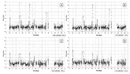
Figure 1.
Initial (raw) and smoothed data of observations of BL Lac object 3C 371 at frequencies 5 and 6.1 GHz, in September 2019, on the 16-m VIRAC antenna (Latvia). (A) 5 GHz, RCP; (B) 5 GHz, LCP; (C) 6.1 GHz, RCP; (D) 6.1 GHz, LCP.
The narrow and sharp peaks in these figures are most likely external interference. The data are smoothed, separately for each observation session, the half-width of the smoothing interval is 10 points, the degree of the polynomial is 3. The average measurement error for the 5 GHz frequency was 0.37 Jy (RCP) and 0.38 Jy (LCP). For the 6.1 GHz frequency, the average error was 0.43 Jy (RCP) and 0.46 (LCP). In parallel, records were kept of the calibration source 3C 295, for control the stability of the receiving. Flux plot of 3C 295 also had minor noise and outliers. An example of 3C 295 recordings at 6.1 GHz in left (LCP) and right (RCP) circular polarizations (September and November–December 2019) is shown in Figure 2.
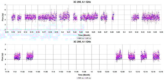
Figure 2.
Plots of stability in the flux density of the calibration radio source 3C 295 based on observations in September and November–December 2019, at a frequency 6.1 GHz.
The linear correlation between the data series was 0.66 for the 5–6.1 GHz (RCP) pair, and 0.57 for the 5–6.1 GHz (LCP) pair. It can be seen that the correlation between the individual frequencies is quite low, but nevertheless, a weak interrelation between the frequencies is possible. This means that the observed variability is most likely caused by an external factor, such as interstellar scintillations of radio emission on inhomogeneities (clouds) of the interstellar medium. To estimate the characteristic time of variations and their form (quasi-harmonic or irregular) for frequencies 5 and 6.1 GHz, spectrograms of each of the circular polarizations were constructed. Previously, the data was interpolated using a cubic spline. The spectrogram plots for the observation session 2–10 September 2019 are shown in Figure 3.
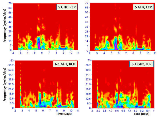
Figure 3.
Spectrograms for 3C 371 (2–10 September 2019). The following plotting parameters were used for the spectrograms: Bartlett spectral window, sliding window width 128 points, spectral window overlap 87%, FFT length-1024 frequencies, visualization in normalized to 0 decibels (dB0). Amplitude color gradations from violet (large amplitude) to blue, green, orange and dark red (background). As can be seen in the figures, variability is present only in the form of short-term irregular variations and a noise component.
The Fourier spectrogram is very convenient for visual assessment of the spectral composition of the data. So, if the data contain quasiperiodic variations, then on the spectrogram they will be seen as straight or curved (if there is a change in the period with time) “ribbons”. Noise components appear as vertical “ribbons”. If the data contain impulse bursts (dips) of the flux density, then on the spectrogram they will be seen as separate “spots” localized in time. For spectrograms, a fast Fourier transform (FFT) calculation in a sliding window is used. In this example, there are the following plotting parameters: Bartlett spectral window, to reduce the effect of “spectral leakage”, the width of the sliding window is 128 points, the spectral windows overlap 87% (necessary to increase the number of segments and the accuracy of the spectrogram, due the length of data series is small), length FFT-1024 frequencies, visualization in normalized to 0 (dB0) decibels: , where are —real and imaginary parts of the FFT transformation, respectively. Analysis of the curves of variations in the emission of extragalactic radio sources using Fourier spectrograms is a typical method in astronomy, which is widely used from radio to X-ray and gamma ranges [10]. Spectrograms for observational data 3C 371 have the usual form for irregular (not quasiperiodic) variations.
Despite the fact, that the flux density variations according to these spectrograms are irregular, it is possible to determine the approximate characteristic time of these variations (since the time points in the spectrogram correspond to the values of the periods). Therefore, a set of “impulse” amplitude bursts visible on the spectrogram correspond to values on the frequency (period) scale (maxima of the FFT spectra in sliding windows). However, these meanings of “periods” are not periods in the usual sense, since the fluctuations are not cyclical, but short-term episodic. Therefore, the below “time scale” of variations shows the average time over which a (non-cyclical) change in the flux density of 3C 371 occurs.
The timescale of irregular variations is approximately 2.6 and 14.6 h for 5 GHz data, and approximately 2.3 and 12.3 h for 6.1 GHz data. The next observation session was 20–21 September 2019 at a single frequency 6.1 GHz. And in this case, only irregular variability plus a quite strong noise was recorded. The characteristic time of flux density variations was approximately 45 min. The next observation session was on 21–25 September 2019 at a single frequency 6.7 GHz. The result was similar to the previous ones. There were only fast irregular variations in the flux density with a noise component. The characteristic time of flux density variations was approximately 41 min. Thus, when observing BL Lac object 3C 371 in the radio range, during September 2019, no manifestations of quasi-harmonic variability were detected at frequencies 5, 6.1, and 6.7 GHz. The nature of the variability of 3C 371 is noisy, without pronounced cyclicity. It should be noted that in September 2019, there were sometimes sharp impulse noise, which somewhat complicates the analysis of the data. Therefore, after a month pause for other scientific tasks, observation sessions of 3C 371 took place in November and December 2019, at frequencies of 5 and 6.1 GHz, on days with good cloudless weather (to minimize atmospheric interference).
So, observations at frequencies of 5 and 6.1 GHz were carried out on 23–25 November and 1–5 December 2019. Longer observations could not be carried out, since 3C 371 is a quite weak radio source, and even a slight cloudiness gives noticeable distortions to the recorded flux density, and autumn and winter at observation point Irbene, contain many cloudy days. The results were similar to the previous ones. No significant variability was found. At the same time, smoothing of the data with a sliding window of 20 points showed that it is possible that the data contain “waves” of variability with an amplitude of approximately 0.5–1 Jy. However, for their more confident selection, at least a week or two of high-quality observations are needed in good weather conditions and with no interference. It is planned to repeat the experiment in the summer months, when there are a large number of clear days in Latvia. Curves of 3C 371 flux density changes (observation sessions on 23–25 November and 1–5 December 2019) at frequencies 5 and 6.1 GHz (initial and smoothed data) are shown in Figure 4.
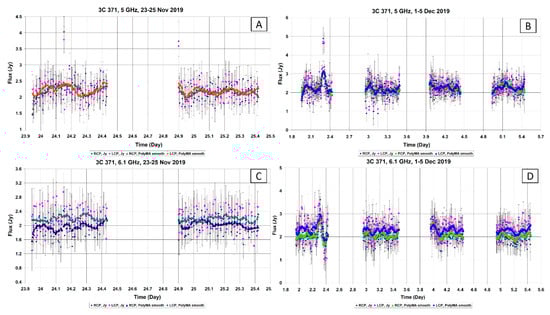
Figure 4.
Curves of 3C 371 flux density changes at 5 and 6.1 GHz, points of the initial data with the “whiskers” of the errors are shown, as well as smoothed curves obtained using the Savitzky–Golay filtration procedure. The sections of the plot show the data. (A) 23–25 November, 5 GHz; (B) 1–5 December, 5 GHz; (C) 23–25 November, 6.1 GHz; (D) 1–5 December, 6.1 GHz.
The average error in measuring the flux density for 5 GHz was 0.37, 0.41 Jy (RCP) and 0.38, 0.42 Jy (LCP) for sessions in November and December, respectively. For a frequency 6.1 GHz, the average flux density measurement error was 0.41, 0.45 Jy (RCP) and 0.46, 0.50 Jy (LCP).
The correlation between the data series, calculated for the smoothed series, shows that on 23–25 November the correlation between frequencies 5 and 6.1 GHz was less than 0.2, which shows that there is no correlation between the data at different frequencies. Moreover, for observations on 1–5 December, the correlation is already higher and amounted to 0.53 (RCP) and 0.65 (LCP) between the frequencies 5 and 6.1 GHz, which shows a possible weak interrelation. However, since the correlation between the frequencies is less than 0.7, interstellar scintillations are most likely causing the observed weak variations in the flux density of BL Lac object 3C 371.
Thus, it can be concluded that intra-day variability in the radio range, of 3C 371 may be present in some observation sessions, but the amplitude of these variations is on average about 0.5 Jy, in rare cases reaching 1 Jy. However, irregular IDV variability may be a feature of the radio source 3C 371. Therefore, for a better understanding of the properties of possible variability, and a more accurate determination of the characteristic times, long-term observations of 3C 371, which, unfortunately, are not so popular among observers, in the radio range are necessary.
To mitigate the effect of random interference, a test technique of “relative” observations was tested in July 2020, without using a calibration radio source. Measurements of the intensity of radio emission in decibels (dB) are obtained relative to the signal of the calibration generator (based on the Zener diode).
Let be Rawon and Rawoff—source measurements with the noise generator turned on and off, respectively (RAW–dimensionless numbers, linearly proportional to the total received power, obtained from the analog-to-digital converter after FFT and averaging). Then, the “relative” intensity of the radio source was calculated as:
where logarithm is decimal.
The use of this technique does not allow obtaining flux density values in Jansky, however, it makes it possible to more accurately check the presence or absence of variability of the investigated radio source, since in this mode there is no need to additionally move the antenna to the calibration source and a section of the sky to obtain a measurement. To reduce noise, each 10 measurements were averaged among themselves. Thus, in one observation session, 800–1800 measurements in dB of the 3C 371 radio source were made. To study the stability of radio receiving in this mode (to make sure that there are no false flux variations associated with instrumental effects), several days of measurements of the Cygnus A (3C 405) calibration radio source were performed. These measurements showed the absence of significant variations in the intensity of the radio emission from the calibration source, which means that there are no supposed instrumental distortions of the observations. On 13 and 14 July 2020, 3C 371source was observed in the “relative” mode. Examples of plots of these observations are shown in Figure 5.
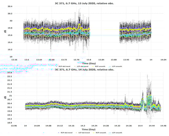
Figure 5.
Plots of “relative” observations of 3C 371, obtained on 13 July (top) and 14 July (bottom) 2020 at a frequency 6.7 GHz. Solid lines-smoothing using the Savitzky–Golay filter with a half-width 10 points of the smoothing window, a polynomial degree is 2, the number of passes 3. As can see in the plots, the intensity variations are almost within the error limits, except for individual episodic bursts. At the end of the observation session on 14 July, high-amplitude impulse bursts (possibly interference) are visible.
As before, the data were smoothed with the Savitzky–Golay filter with a half-width 10 points of the window and degree 2 of polynomial, to highlight the intensity variations against the background noise.
Observations, smoothed by the Savitzky–Golay filter, show irregular variations with low amplitude, close to the measurement error. With the exception of individual, short-term impulse bursts, there is no intra-day variability in 3C 371. However, the example of the 14 July recording, shows an increase in the radio intensity with a maximum at 2 h 30 min local time (in a 24-h format) (or 14.104388 in fractions of a day) with a change in intensity at 0.33 dB or power of 1.08 times. The largest change in burst intensity was approximately 1.08 dB or 1.28 times in power (10 h 19 min local time or 14.430399 in fractions of a day). And on the record on 13 July, the largest burst of intensity occurred at 18 h 28 min local time (or 13.769802 in fractions of a day) (the change in intensity was approximately 0.30 dB or 1.07 times). Similar measurements were carried out at two frequencies 5 and 6.1 GHz on 18 and 19 July 2020. The intensity of 3C 371 radio emission in these cases changed very slightly.
In this case, to determine whether there is variability in the studied data (in other words, whether there is a “memory effect” in the data in the form of repeatability or trend changes in data), the method of calculating the Hurst exponent was applied (detailed description, for example, in [11]). This method is convenient for a rough understanding of the presence or absence of cyclical or trend variability, hidden by noise. If H = 0.5, the data is white noise, if H < 0.5, the data series is anti-constant (any tendency tends to change the opposite) and each data value is likely to have a negative correlation with the previous values. If the time series has “memory”, that is, subsequent values depend on the previous ones, which is a normal consequence of variability, the values of the Hurst exponent tends to 1. Usually, when H value equal to, or greater than 0.8, indicates a pronounced “memory effect”, or the presence variability in the time series.
For example, for the session on 18 July 2020, frequency 5 GHz, Hurst exponent values: H = 0.914 ± 0.0068 (LCP); H = 0.952 ± 0.0122 (RCP) correspond to the presence of irregular variability in this observation session. For 6.1 GHz on the same date: H = 0.714 ± 0.0028 (LCP); H = 0.748 ± 0.0036 (RCP). It can be seen that at a frequency 6.1 GHz, the “memory effect” is less pronounced, but nevertheless a weak variability is present. And already for the data on 19 July 2020, the situation is different. At a frequency 5 GHz, Hurst exponent value: H = 0.593 ± 0.0043 (LCP); H = 0.641 ± 0.0098 (RCP), which shows a weak interrelation of subsequent intensity values with previous ones, and there is practically no variability. At 6.1 GHz for 19 July, the values: H = 0.466 ± 0.0065 (LCP); H = 0.430 ± 0.0087 (RCP), which shows the closeness of the time series to anti-constant noise. This is confirmed by the statistical Kolmogorov and Smirnov tests for checking the “normality” of the distribution [12]. Thus, if on 18 July there may have been weak variability, then on 19 July it was replaced by noise variations in the intensity of 3C 371 radio emission.
An example of the Kolmogorov and Smirnov test result, about observational data normality, 5 GHz (RCP), for 18 and 19 July 2020 is shown in Table 2. The threshold value was 0.05. However, statistical tests for the normality of distribution, for radio observations, have limited applicability, since the presence of interference in the data against the background of noise can lead to a false negation about normality of the data distribution. Therefore, interference removal is an important task.
Table 2.
The table shows examples of Kolmogorov and Smirnov tests of (statistics, two-sided p-value and output), for 18 and 19 July 2020 at 5 GHz (RCP) (threshold value is 0.05). As can see, on 19 July the data had a normal distribution, but not on 18 July.
Thus, the experiment using measurements in decibels, showed the absence of reliable variability of 3C 371 radio emission at frequencies 5 and 6.1 GHz. However, in some sessions, there may be variations in the intensity with low amplitude, and sharp episodic noise-like type bursts, were also observed.
From 22 to 28 July 2020, on the 16-m antenna, the flux density measurement mode in Jansky, at frequencies 5 and 6.7 GHz was again used and observations of the radio source 3C 371 continued. The plots of the initial and smoothed observations of the 3C 371 source (sessions 22 and 25–28 July 2020), at frequencies 5 and 6.7 GHz, are shown in Figure 6.
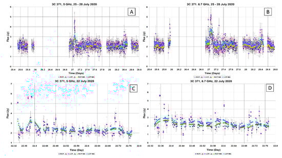
Figure 6.
Plots of flux density variations of 3C 371, 22 July 2020 at 5 GHz (C) and 6.7 GHz (D), as well as plots of flux density variations from 25 to 28 July 2020 at 5 GHz (A) and 6.7 GHz (B). The figures also show smoothed data, for left (LCP) and right (RCP) circular polarizations. It can be seen that the amplitude (for smoothed data) of irregular variations in the flux density almost does not exceed 0.5 Jy, with an amplitude of bursts, about 1 Jy, as in other observation sessions.
The average flux density for 25–28 July, at a frequency 5 GHz, was 2.118 ± 0.420 Jy (RCP) and 2.127 ± 0.418 Jy (LCP). Over the same time interval, at a frequency 6.7 GHz, the average flux density was 2.145 ± 0.451 Jy (RCP) and 2.287 ± 0.480 Jy (LCP).
To estimate the characteristic time of variations, we construct Lomb–Scargle power spectra (using smoothed data) in a double logarithmic scale with confidence levels of probability (a double logarithmic scale is needed to clearly see the entire LS power spectrum). An example of periodograms (with a Bartlett spectral window, to reduce the spectral leakage effect) for non-uniform time series (observation session on 25–28 July 2020) is shown in Figure 7.
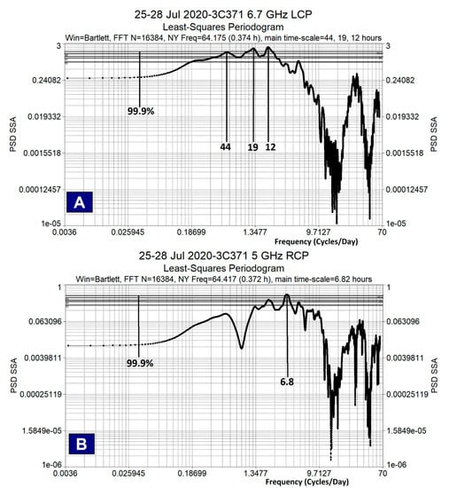
Figure 7.
Examples of periodograms for the observation session of 3C 371 source, 25–28 July 2020. (A) shows the periodogram (spectrum length 16384, Nyquist frequency 64.175 cycles/day, which corresponds to a period 0.374 h) for left circular polarization at 6.7 GHz (typical variation times are approximately 44, 19, 12 h). (B) shows the periodogram (spectrum length 16384, Nyquist frequency 64.417 cycles/day corresponding to a period 0.372 h) for right-hand circular polarization at 5 GHz (characteristic time 6.82 h).
This example shows that, above the 99.9% confidence level, the characteristic time of flux density variations at a frequency 5 GHz is ≈ 4.7 h (LCP) and ≈ 6.8 h (RCP). Some closeness of these values to the 4 and 6 h daily harmonics can be seen. As can be seen, on the time scales the variations differ for two circular polarizations, with a correlation coefficient 0.83, between two circular polarizations. Quite different characteristic times of flux density variations for 6.7 GHz. For both polarizations, they were ≈ 19 and 12 h, and in addition, in the left polarization, a maximum of the periodogram is visible, corresponding to variations with a characteristic time ≈ 44 h (the maxima of the periodograms are at 99.9% and slightly more). This is close to twice (48 h) the daily 24 h period, 12 h is the harmonic of the daily period, and the 19 h variation can be a distorted daily period, which needs additional verification on more intensive observations of at least one week in duration.
3.2. Optical Observations
Observations of 3C 371 on the AZT-3 telescope with a mirror diameter 48 cm (Mayaki Observatory (Odessa I.I.Mechnikov University), Ukraine) were carried out in the time interval from 8 September to 12 October 2019 in filters V, R. On 7–20 October 2019, the Vihorlat observatory (Slovakia) joined the observations using the VNT telescope (mirror diameter 1 m) and V, R, I filters. Observations at the Baldone Observatory (Latvia) on the Schmidt camera with a mirror diameter 1.2 m were carried out on 24, 27 October and 9 December 2019 using R filter. The neighborhoods of 3C 371, marked with the target object of observation and comparison stars are shown in Figure 8.
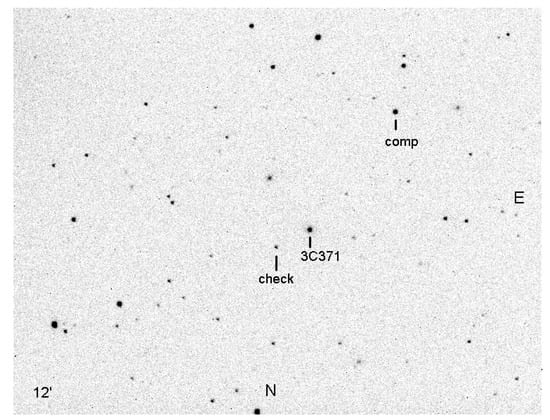
Figure 8.
Neighborhoods of BL Lac object 3C 371, the figure also shows the comparison star and the checking star, as well as the directions to the North and East.
The standard reduction of the CCD frames were carried out by using the MUNIPACK (http://sourceforge.net/projects/c-munipack) software. The procedures for an aperture photometry is composed of the dark-level and flat-field corrections, determination of the instrumental magnitudes and precision. The photometry was transformed to the standard VRI Johnson-Cousins system by means of the differential photometry method [13]. Observations with the AZT-3 telescope are reduced to the standard photometric system using the following formulas:
where denotes stellar magnitudes in the standard system, the difference between the magnitudes of the variable star and the comparison star, thecolor transformation coefficients, the difference between the color indices of the variable star and the comparison star, and the magnitudes of the comparison star in the standard system.
The transformation coefficient was determined from observations of standard stars [14].
The weak foggy halo of the host galaxy, where the 3C 371 source located, was not specially taken into account, because it is simply not visible on the CCD matrices installed on the telescopes, as can be seen in Figure 8, the image from the CCD matrix of the AZT-3 telescope, where the source 3C 371 is does not differ from nearby stars.
Light curves of the source 3C 371 were observed with telescopes AZT-3 (Ukraine) and VNT (Slovakia) and are shown in Figure 9, in bands V, R (AZT-3) and V, R, I (VNT).
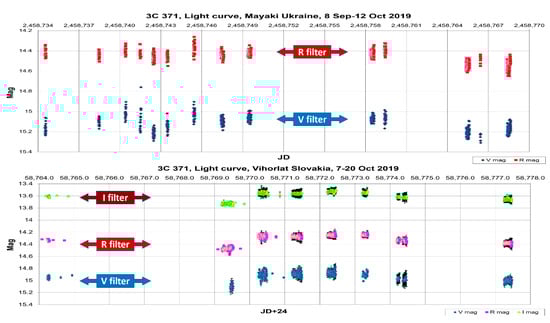
Figure 9.
Light curves of 3C 371, obtained in Ukraine (upper graph) and Slovakia (lower graph). The flags indicate the V, R, I bands for the individual light curves.
According to the Baldone Observatory, intra-night trends were observed for two days, and for one night on 24 October, there was close to quasiperiodic variability. Observatory plots at Baldone Observatory (24, 27 October and 9 December 2019) in the R-band are shown in Figure 10.
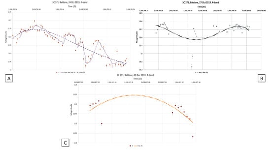
Figure 10.
Light curves for three nights (24 (A), 27 (B) October and 9 December (C) 2019) obtained at the Baldone Observatory. The polynomial trends are plotted in the data, showing the brightness variations of 3C 371 during these individual nights of observations.
The amplitudes of variability in fractions of a magnitude, according to observations at the Mayaki, Vihorlat, and Baldone observatories, are shown in Table 3. Filters in which the observations were made, are indicated in brackets. For the data of the Baldone observatory, the dates of observation nights, in the R filter, are also shown.
Table 3.
Table of variability amplitudes and errors (in fractions of magnitude) of observations of the 3C 371 source at the observatories in Ukraine, Slovakia and Latvia at 2019.
To analyze the variability, the Lomb-Skargle periodograms were constructed for the observations of the Mayaki and Vihorlat observatories. In the case of the Vihorlat observatory, the main peak in periodograms corresponded to a period value 6.8 days. There were also split maxima with close values, about 1.1 and 0.9 days (probably, the contribution of the diurnal harmonic, which is not related to the variability of 3C 371).
To refine this result, single sinusoids were inscribed into the light curves using the least squares method. The method of data approximation by a trigonometric polynomial (Fourier decomposition) for estimating the values of the periods of cyclic variations in time series of extragalactic sources observations, is far from new and its widely used, for example, in the analysis observations of variable stars [15]. The algorithm creates a parametric time series model, consisting of sinusoids or damped sinusoids, and is made from several parts. First, the Lomb–Scargle method is used to estimate the frequencies and the number of sinusoids. A linear approximation is then performed to determine the phases and amplitudes of the sinusoids, which are used as starting values. The final stage uses these initial values to optimize the resulting time series model, using the least squares the Levenberg–Marquardt iterative method, which refines the previously obtained values of frequencies, phases and amplitudes of sinusoids, by fitting the model to the best approximation of the initial data [16]. The refined period values of the main sinusoids (which make the main contribution to the observed variations) can be considered as the estimated values of the quasiperiods, contained in the light curves of the extragalactic radio source 3C 371. However, in this case, when there are few observation sessions, even the approximation by 1–3 sinusoids allows to approximately estimate the quasiperiods in the case of cyclicity.
Thus, the following values of the sinusoids periods, were obtained, which provided the best approximation of the initial data: 7.3 days (I), 7.2 days (R), 7.5 days (V).
In the case of Mayaki Observatory, the light curves contain two components, which have the following periods values of the approximating sinusoids: 6.6 days and 4.6 days (V); 6.5 days and 4.4 days (R). However, due to the large gaps in the data, about 4 day cycle cannot yet be considered reliably determined and requires further verification. Weak trends are also visible, for which estimation of the characteristic time (by inscribing a segment of a sinusoid, by the least squares method) is 35.6 days (V) and 67.8 days (R). As can be seen, there is a significant difference between the estimates of characteristic time for the trend change in brightness of 3C 371 in the V, R filters. Longer observations with smaller gaps between sessions are required to reliably determine the time scale of trend brightness variations. Examples of periodogram and sinusoidal fit for 3C 371 observations at Mayaki and Vihorlat observatories are shown in Figure 11.
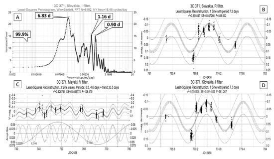
Figure 11.
(A) shows an example of periodogram for observations at the Vihorlat observatory (I). It can be seen that the main maxima exceed the 99.9% confidence level (which means that only 1 from 1000 sets of noise, can accidentally give a maximum with this height). (C) shows an example of a trigonometric polynomial drom 2 sinusoids, plus a trend segment for observations at the Mayaki Observatory (V). (B,D) show examples of fitting 1 sinusoid into the data series, R and I, respectively. In this example, the approximation parameters, R2 = 0.62, SE = 0.047 (standard error of approximation), F-statistics (Fisher) = 128.48 (C); R2 = 0.69, SE = 0.047, F = 556.63 (B); R2 = 0.70, SE = 0.041, F = 581.26 (D).
This figure shows the values of the periods of the peaks of the Lomb-Scargle periodogram for the filter I data (Vihorlat observatory), as well as three graphs (Mayaki and Vihorlat observatories) with the approximation of the original data by sinusoids. It can be seen, for example, the initial value of the period of 6.83 days (I) was refined to the value of 7.3 days by fitting the sinusoid to the data using the least squares method. This figure also shows the parameters of the approximation (coefficient of determination R2, standard error SE и F-Fisher statistics) which shows good reliability of the found periods values. The values of approximation parameters are shown in the caption to Figure 11.
Consideration of a longer data series (2018–2020) of 3C 371 observations, obtained in the V filter, from a free observational database AAVSO (American Association of Variable Star Observers, https://www.aavso.org/) showed the presence of only trend changes in brightness without a cyclical component. After a big drop, the overall brightness increase began in October 2019. The long-term light curve of 3C 371 source, as observed by the AAVSO, for the time interval 2018–2019 in the V band, is shown in Figure 12, as well as the inscribed 5-degree polynomial, showing a slow, wavy brightness change of 3C 371 throughout the year.
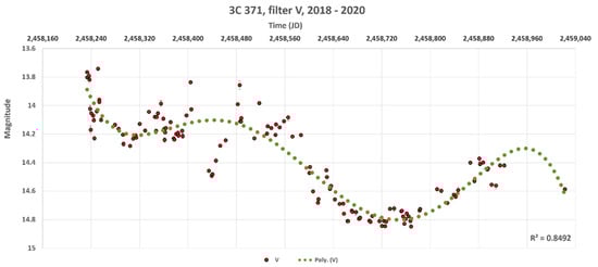
Figure 12.
Long-term light curve of 3C 371 in the V-band, obtained in the time interval 2018–2020 (observations from AAVSO database). A wavy long-term trend is visible (polynomial degree is 5).
The minimum characteristic variability time, according to observations at the Mayaki observatory was 2.8 h (V) and 3 h (R). For observations at the Vihorlat observatory, the minimum characteristic variability time is 2.3 h (V), 2.2 h (R), and 2.6 h (I). Within individual nights, there were either noisy brightness variations or irregular ones. Similar observations of 3C 371 at the KittPeak observatory, published in 1978, showed similar properties. There were noise brightness variations within individual nights [17]. In an earlier work, it was shown that within individual nights, 3C 371 exhibits significant irregular variability [18]. It seems that events of significant variability within the night are less frequent than manifestations of noise-like variability.
In the case of observations at the Baldone Observatory, on one night of observations, 24 October 2019, brightness fluctuations close to quasiperiodic were observed. An example of the approximation of the 3C 371 light curve (24 October 2019) by a trigonometric polynomial from two sinusoids—a sinusoidal trend segment and a main sinusoid, is shown in Figure 13.
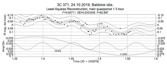
Figure 13.
An example of fast brightness variations for 24 October 2019, in the R filter, observed at the Baldone observatory. Shown is a trigonometric polynomial approximation from 1 sinusoid with a period 1.3 h, plus a trend sinusoidal segment (showing a decrease in brightness during the night) with a period 7.6 h. This value (7.6 h) is very close to the 8 h diurnal harmonic, so it most likely cannot be considered a correct result. Approximation parameters: R2 = 0.83, SE = 0.033, F = 62.70.
The value of the estimated quasiperiod is 1.3 h. In this case, rapid brightness fluctuations are superimposed on the trend decrease of brightness. Sinusoidal trend segment has a characteristic time 7.6 h, but this is very close to value of the 8 h diurnal harmonic, and therefore, in this case, the value of characteristic time of brightness variations cannot be considered as correct result. However, on individual nights of observations in Ukraine and Slovakia, apart from trends, no such brightness variations were observed, only irregular variability. Therefore, this result requires further verification by new optical observations.
Additional observations carried out in May and July 2020 (Slovakia, Vihorlat Observatory) also showed the presence of day-to-day variability, but only four nights of qualitative observations were obtained on 21 May and 1, 5, and 7 July. The common plot of 3C 371 observations in May and July 2019 is shown in Figure 14, bands V, R, I (obtained at VNT telescope).
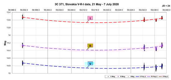
Figure 14.
Light curve of 3C 371 observations, obtained at the Vihorlat observatory in filters V, R, I. Dotted trend lines-polynomials of 2 degree.
A separate plot for an example of 3C 371 variability inside the night 1 July 2020 (bands V, R, I) is shown in Figure 15.
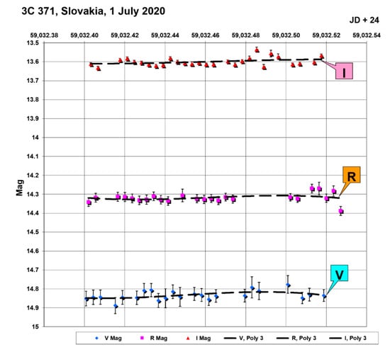
Figure 15.
An example of light curves inside the night of 1 July 2020 in filters V, R, I (Vihorlat observatory). Dotted trend lines—third degree polynomials. Weak brightness variations are seen in the V and R bands with a characteristic time of about 20 min.
Table 4 presents the amplitudes of variability and measurement errors for the observation session of 3C 371 source at the Vihorlat observatory, carried out in the time interval from 21 May to 7 July 2020, in the V, R, I filters.
Table 4.
Table of amplitudes and measurement errors (in fractions of magnitude) for observation session of 3C 371 source, performed at the Vihorlat observatory, on 21 May and 1, 5, 7 July 2020.
As can be seen from this example, in most cases, the amplitude of the observed variability within the night is close or comparable to the average observational error. Therefore, one can say that significant variability within the night occurred on 1 and 7 July. On other days, brightness variations are poorly distinguishable against the background of the measurement error.
However, day-to-day brightness variations in the V, R, I bands are well distinguishable; however, these observations are insufficient to accurately determine the characteristic variability time. However, it can be roughly estimated by writing segment of a sinusoid into the data for 1, 5, 7 July, using the least squares method. Its period is approximately 5.2 days for the V band, and 5.0 days for the R band. In the I band, the approximation error was too large.
The total amplitude of variability for four days was:
0.184m (V), 0.160m (R) and 0.125m (I) with an average error 0.032m (V), 0.036m (R) and 0.022m (I). Thus, BL Lac object 3C 371 has day-to-day variability. However, to determine its cyclicality, or the absence of cyclicality, more data are needed, which are planned to be obtained in the next observation session at the observatories in Slovakia, Ukraine, and Latvia.
To confirm or disprove the presence of quasiperiodic cyclic variations with a period value about 7 days in the 3C 371 optical observation data, the data of all different 3C 371 observation sessions performed on the AZT-3 telescope (Mayaki observatory, Ukraine) were combined from 3 September 2019 to 30 January 2020, in the V, R filters. The obtained light curves are shown in Figure 16. This figure shows a rather rapid increase in brightness by more than 0.5 magnitude, from the average brightness, to 27 October 2019.
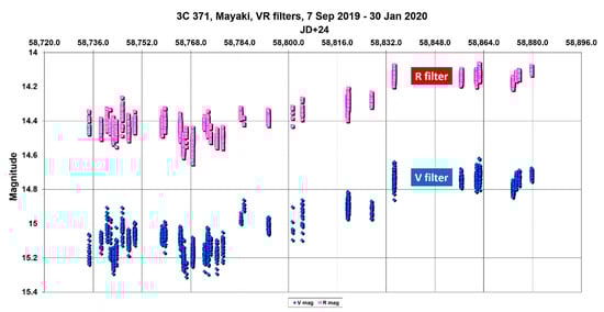
Figure 16.
Common light curves of the source 3C 371, obtained at the Mayaki observatory (Ukraine) in V, R bands, during the time interval 7 September 2019–30 January 2020.
Descriptive statistics of these obtained time series of observations in Mayaki observatory are shown in Table 5.
Table 5.
The values are shown—mean, median, standard deviation, maximum, minimum and number of data points, for observations of 3C 371 in the time interval 7 September 2019–30 January 2020, on the AZT-3 telescope, Mayaki observatory (Ukraine).
Next, a digital spectral analysis was carried out using the Lomb-Scargle method and time series models were obtained in the form of trigonometric polynomials from four sinusoids (V band) and five sinusoids (R band). An example, for the V band, is shown in Figure 17. The figure shows a parametric spectrum (top panel) showing the initial values of quasi-periods, identified by the Lomb–Scargle method for non-uniform time series, the middle panel shows an optimized (least squares method) trigonometric polynomial, a time series model from four sinusoids (one trend segment of a sinusoid, describing a slow brightness change and three target sinusoids, describing fast brightness variations of 3C 371), and the bottom panel of Figure 17 shows sine waves, components of a trigonometric polynomial. Frequency values in cycles per day.
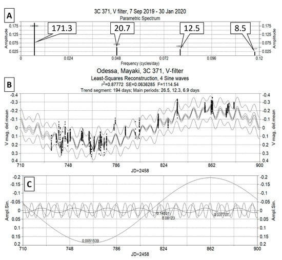
Figure 17.
Result of the analysis of cyclical variability in the light curve of 3C 371 in the V filter (7 September 2019–30 January 2020), according to observations in the Mayaki observatory (Ukraine). (A) Parametric spectrum with periods values of 4 sinusoidal components in the time series, flags show the initial values of quasiperiods in days; (B) Approximation of the original observational data (the average value is subtracted), by a trigonometric polynomial from 4 sinusoids (where 1 segment of the sinusoid shows a slow trend change in brightness) that were fitted to the original data, using the least squares method, and accordingly, the values of periods for each sinusoids were refined; (C) This panel shows the sinusoidal components, which formed the approximating trigonometric polynomial. Thus, the following values of estimated quasiperiods were obtained: 26.5, 12.3, and 6.9 days. The estimated characteristic time of trend change in brightness of 3C 371, in this example, was about 194 days. The quasiperiod 6.9 days (very close to value 7 days, obtained earlier) was preserved in a longer series of data, which confirms the correctness of its determination.
As can be seen from the example in Figure 17, the data contains a quasiperiod 6.9 days, which is close to the values of the main quasiperiod, about 7 days, obtained earlier, when analyzed shorter data series from the Mayaki and Vihorlat observatories. In addition to the previously found quasiperiod, quasiperiods with values 12.3 and 26.5 days appeared. Moreover, 26.5 days is close to quadruple 6.9 days (27.6 days) and looks like it is harmonic of this main quasiperiod. The quasiperiod 12.3 days may be real, but to test this assumption, better quality series of observations are needed, with smaller data gaps (which are expected to be obtained in the next stage of this work). The characteristic time of trend change in the brightness of 3C 371 source, estimated as the period of sinusoidal segment, is 194 days. The following parameters of approximation by a trigonometric polynomial are obtained: R2 = 0.878, SE = 0.064, F = 1114.54. As can see from this example, the coefficient of determination is quite close to the value of 0.9, which shows a very good agreement between the fitting curve and the original data, and high value of the Fisher statistic also confirms the very good quality of the data approximation by four sinusoids. Thus, it is almost confirmed that the 6.9 days quasiperiod is true and actually describes fast inter-day brightness variations of the 3C 371 source in the optical range.
Analysis of the 3C 371 light curve in the R-band, showed fairly similar results. Thus, the characteristic time of the trend change in brightness of 3C 371 in the R band was about 172 days, the values of other found quasi-periods were 20.6, 13.2, and 7.7 days. This is quite close to the results, obtained from observations in the V filter. However, an additional harmonic with a period 38.3 days appeared in the R-band, which is very close to the fivefold increased value (38.5 days) of the main quasiperiod 7.7 days, so this is most likely the harmonic of the main quasiperiod. In the same way, the value of quasiperiod 20.6 days is close to the triple value (23.1 days) of the main quasiperiod in the R-band. The value of quasiperiod 13.2 days is possibly real, but its differences from the value 12.3 days obtained in the V-band, indicate the need for clarification by further observations.
4. Discussion
The fact that the extragalactic source 3C 371 is optically variable was noted as early as the 1960s. For example, it was shown in [19] that a change in brightness by approximately one stellar magnitude occurred over a time interval about two years of observations, and low-amplitude changes in brightness by 0.10–0.15 stellar magnitude occur over a time interval of several days. Some general information on the fast optical variability of 3C 371 with an amplitude about 0.5 magnitude is given in [20].
The quasiperiodic activity of BL Lac object 3C 371 in the optical range was recorded in the early work [21], where the presence a period 163 days is noted, as well as the similarity shape of the light curve for different components of brightness variations with different time scales. When observing 3C 371 in the X-ray range on the Exosat satellite, intra-day variability was detected with characteristic times from 8 h to 25 min. The rapid variability of such a time scale, in the X-ray range, is in good agreement with the model of an inhomogeneous synchrotron flow with Compton backscattering [22]. Low-amplitude intra-day optical variability (filter V) for 3C 371 was recorded in [23]. On some nights, linear trends of an increase or decrease in brightness were seen. In newer optical observations (filters B, I), it was confirmed that 3C 371 has significant low-amplitude variability on a time scale from several hours to several days. Moreover, there is a strong correlation between the B and I bands on short and long time scales [24].
On the whole, different authors at different times have observed fast optical brightness variations with a characteristic time of less than a few hours. However, for the radio range, there are quite a few works devoted to the intra-day variability of 3C 371.
Observations with the aim of searching for intraday variability of 3C 371 in the radio range at frequencies 5, 6.1, 6.7 GHz, at the 16-m VIRAC radio telescope, were carried out at different times, in September, November and December 2019 and also in July 2020. It is shown that the obtained data series contain weak variations in the flux density with an amplitude about 0.5 Jy, less often 1 Jy, and the nature of variability is completely irregular, without any quasiperiodic manifestations. The observations on 2–10 September were slightly distorted by impulse noise, while the 6.7 GHz observations on 21–25 September were quite noisy. Better observations were in November and December. Also, they did not show significant quasi-harmonic variability, only low-amplitude irregular variations in each of the sessions. Long-term trend changes in the flux density 3C 371 were also not found in the studied time interval. Observations in the radio range in July 2020 showed an ambiguous result. On some days, the radio source showed only noise variations, on some days there were irregular low amplitude variations. No quasiperiodic flux density variations were detected. Thus, the irregular intra-day low-amplitude variability in the radio range in 3C 371 is most likely present, more or less, in different observation sessions, however, its reliable select and assessment of properties, requires long-term observations for several weeks or, even better, months.
At the same time, optical observations at the observatories Mayaki (Ukraine), Vihorlat (Slovakia) and Baldone (Latvia), carried out on 8 September–12 October (Mayaki), 7–20 October (Vihorlat), 24, 27 October, and 12 December (Baldone) 2019 in filters V, R, I showed significant variations in the brightness of 3C 371 within observation nights, as described in the early works of other authors. Analysis of the light curves showed the presence of quasiperiodic changes, with a main period about seven days and a pronounced diurnal modulation. This quasiperiod was obtained for observations over different time intervals, both in Slovakia and in Ukraine (the distance between the observatories is about 900 km). This confirms the reality of the found quasiperiod in the optical range, and when analyzing the works of other authors, the presence of seven-day quasiperiod, was not previously noted. Thus, the result obtained is new. In addition, according to the longer light curves in the V, R filters obtained at the Mayaki observatory, there may be additional cyclicity with a characteristic time 4.6 days, but quite large gaps between observations, do not allow it to be reliably distinguished. At 24 October, according to observations at Baldone in the R filter, showed a nearly quasiperiodic brightness change with a characteristic time about 1.3 h. Observations carried out in May and July 2020 showed that the optical brightness of 3C 371 changes, with an assumed characteristic time of about five days, at this time interval, but this is a quite rough estimate due to the small number of observations.
Analysis of the total light curves, the longest, in our study, observations obtained in the V, R bands at the Mayaki observatory (Ukraine) in the time interval from 7 September 2019 to 30 January 2020, showed, that presence of a quasiperiod about seven days, obtained earlier is confirmed by longer observations. The estimated characteristic time of the trend change in brightness of 3C 371 was 194 days (V band) and 172 days (R band), which is quite close to the result obtained in a much earlier work (M.K. Babadzanjanz, E.T. Belokon 1975) [21], where the quasiperiod value was 163 days in B-band (1966–1973). Thus, in this work, the presence of regular brightness variations of 3C 371 source, with a period quite close to 160 days, is possibly partially confirmed.
Thus, quasiperiodic variations in the emission of BL Lac object 3C 371 were observed in the optical range, but were completely absent in the radio range. Since the correlation between radio frequencies 5 and 6.1 GHz is quite low and generally lower than 0.7, the observed variations are most likely caused by the interstellar medium (refraction of radio emission into inhomogeneities of a galactic interstellar medium), which is considered, for example, in [25]. Since 3C 371 has a well-defined optical jet with bright moving components in it, it can be assumed that the observed cyclic variability in the optical range is caused by quasi-regular processes in the jet. Some authors associate the fast optical variability of active galactic nuclei with unstable processes in the accretion disk, as, for example, in [26]. However, in the case BL Lac objects like 3C 371, due to the small angle between the jet and the line of sight, the main contribution to the observed inter-day variability and variability during individual nights should be made by processes in the jet, such as shock waves interacting with local inhomogeneities in the jet, which can cause variations within the night, and longer brightness variations on time scales of about several days are possibly associated with small-scale disturbances within the jet [27,28].
5. Conclusions
Observations of 3C 371 radio source, in the radio range on the 16-m VIRAC antenna (Latvia), at frequencies of 5 and 6.1 GHz, (the observation sessions were in September, November, and December 2019 and July 2020) showed the presence of only irregular variations in the flux density. The timescale of these variations is approximately 2 h and 12–14 h. The correlation between frequencies 5 and 6.1 GHz is quite weak, i.e., 0.5–0.6 and less than 0.2 in some observation sessions. There is a weak correlation between the frequencies 5 and 6.1 GHz in individual observation sessions. Observations on 22, 25–28 July, at frequencies 5 and 6.7 GHz showed the probable presence of flux density variations with characteristic times close to 5 and 7 h at a frequency 5 GHz, and at 6.1 GHz, manifestations of semidiurnal 12-h harmonic were observed. The linear correlation between 5 and 6.7 GHz using a smoothing data filter was 0.62 (5 GHz RCP vs. 6.7 GHz RCP) and 0.65 (5 GHz LCP vs. 6.7 GHz LCP). Despite the existing weak interrelation between the frequencies in this observation session, the characteristic times of flux density variations at different frequencies are differ.
Smoothing the radio data for individual observation sessions using the Savitzky–Golay filter, showed the possible presence of low-amplitude waves (0.5 Jy, rarely up to 1 Jy) of irregular flux variations; however, the observation duration was insufficient to reliably determine the amplitude of these variations, against the noise background.
Optical observations of 3C 371 were carried out at the observatories Mayaki (Ukraine), Vihorlat (Slovakia), Baldone (Latvia), the observation sessions were in September, October, and December 2019, and additionally in May and July 2020. In the optical range (bands V, R, I), a close to quasiperiodic changes in the brightness of 3C 371 with a characteristic time of about seven days was found, according to data from observatories in Ukraine and Slovakia. In the optical range, the 3C 371 shows changes in brightness during individual nights, in the form of trend variations. There is no correlation between radio and optical observations at overlapping time intervals. Analysis of longer light curves in V and R bands, obtained at the Mayaki observatory (Ukraine) over the time interval 7 September 2019–30 January 2020, confirmed the presence of a main period, with a value close to seven days, in both bands. On 24 October 2019, according to observations at the Baldone observatory (R-band), the variability during the night was close to quasiperiodic with a characteristic time of about 1.3 h.
As a result, it can be noted that, in the radio range, during the observation time interval, there is no cyclic variability of 3C 371 (however, low-amplitude irregular flux density variations are often present), but there is cyclic variability in the optical range, including fast intra-night brightness variations. Since the flux density variations in the radio range are quite weak, in the future, it is planned to carry out longer quasi-continuous and multifrequency observations of the 3C 371 on the 32-m VIRAC (Latvia) antenna, in order to refine the obtained results.
Author Contributions
Original draft writing and all processing and analysis of observational data, A.S.; review and editing, M.R. and V.B.; optical observations at Mayaki observatory (Ukraine), S.U. and L.K.; optical observations at Vihorlat observatory (Slovakia), I.K. and P.D.; optical observations at Baldone observatory (Latvia), I.E.; radio telescope control and writing control scripts, A.O. and M.B. All authors have read and agreed to the published version of the manuscript.
Funding
The contribution of Artem Sukharev has been funded by ERDF postdoctoral grant No. 1.1.1.2/VIAA/2/18/363 “Investigation of intra-day and inter-day variability of various types of extragalactic radio sources using telescopes of the Ventspils International Radio Astronomy Centre (RISE)”. Project is being implemented in Ventspils University of Applied Sciences.
Acknowledgments
The authors would like to thank the VIRAC engineering team for their help in obtaining radio data. We thank the referees for their useful suggestions which helped to improve quality of the paper.
Conflicts of Interest
The authors declare no conflict of interest.
References
- Perlman, E.S.; Padgett, C.A.; Georganopoulos, M.; Sparks, W.B.; Biretta, J.A.; O’Dea, C.P.; Baum, S.A.; Birkinshaw, M.; Worrall, D.M.; Dulwich, F.; et al. Optical Polarimetry of the Jets of Nearby Radio Galaxies. I. The Data. Astrophys. J. 2006, 651, 735–748. [Google Scholar] [CrossRef][Green Version]
- Pesce, J.E.; Sambruna, R.M.; Tavecchio, F.; Maraschi, L.; Cheung, C.C.; Urry, C.M.; Scarpa, R. Detection of an X-Ray Jet in 3C 371 with Chandra. Astrophys. J. Lett. 2001, 556, L79. [Google Scholar] [CrossRef]
- Usher, P.D.; Manley, O.P. The Unusual Long-Term Behavior of 3c 371. Astrophys. J. 1968, 151, L79–L82. [Google Scholar] [CrossRef]
- Itoh, R.; Nalewajko, K.; Fukazawa, Y.; Uemura, M.; Tanaka, Y.T.; Kawabata, K.S.; Madejski, G.M.; Schinzel, F.K.; Kanda, Y.; Shiki, K.; et al. Systematic study of Gamma-Ray bright blazars with optical polarization and Gamma- Ray variability. Astrophys. J. 2016, 833, 77. [Google Scholar] [CrossRef]
- Bleiders, M.; Bezrukovs, V.; Orbidans, A. Performance evaluation of Irbene RT-16 rado telescope receving system. Latv. J. Phys. Tech. Sci. 2018, 54, 42–53. [Google Scholar]
- Bromba, M.U.; Ziegler, H. Application hints for Savitzky–Golay digital smoothing filters. Anal. Chem. 1981, 53, 1583. [Google Scholar] [CrossRef]
- Baba, T. Time-Frequency Analysis Using Short Time Fourier Transform. Open Acoust. J. 2012, 5, 32–38. [Google Scholar] [CrossRef]
- Zhang, W.J. The Research of the NURBS Curve Interpolation Algorithm. Adv. Eng. Forum 2011, 2–3, 614–618. [Google Scholar] [CrossRef]
- VanderPlas, J.T. Understanding the Lomb-Scargle Periodogram. Astrophys. J. Suppl. Ser. 2018, 236, 16. [Google Scholar] [CrossRef]
- Smigiel, E.; Knoll, A.; Broll, N.; Cornet, A. Determination of layer ordering using sliding-window Fourier transform of x-ray reflectivity data. Model. Simul. Mater. Sci. Eng. 1998, 6, 29–34. [Google Scholar] [CrossRef]
- Cadenas, E.; Campos-Amezcua, R.; Rivera, W.; Espinosa-Medina, M.A.; Méndez-Gordillo, A.R.; Rangel, E.; Tena, J. Wind speed variability study based on the Hurst coefficient and fractal dimensional analysis. Energy Sci. Eng. 2019, 7, 361–378. [Google Scholar] [CrossRef]
- Simard, R.; L’Ecuyer, P. Computing the Two-Sided Kolmogorov–Smirnov Distribution. J. Stat. Softw. 2011, 39, 1–18. [Google Scholar] [CrossRef]
- Benson, P.J. Transformation Coefficients for Differential Photometry. Int. Amat. Prof. Photoelectr. Photom. Commun. 1998, 72, 42. [Google Scholar]
- Udovichenko, S.N. Investigation of the Photometric System of CCD-Photometer and the AZT-3 Telescope. Odessa Astron. Publ. 2012, 25, 32. [Google Scholar]
- Deb, S.; Singh, H.P. Light curve analysis of variable stars using Fourier decomposition and principal component analysis. Astron. Astrophys. 2009, 507, 1729–1737. [Google Scholar] [CrossRef]
- Hoffman, D.I.; Harrison, T.E.; McNamara, B.J. Automated Variable Star Classification Using Northern Sky Variability Survey. Astron. J. 2009, 138, 466–477. [Google Scholar] [CrossRef]
- Miller, H.R.; McGimsey, B.Q. Photoelectric intraday observations of BL Lacertae, 3C 66 A, B2 1652+39, and 3C 371. Astron. J. 1978, 220, 19–24. [Google Scholar] [CrossRef]
- Urasin, L.A.; Lavrova, N.V. Short-period brightness variations of the nuclei of the N-galaxies 3C 371 and 3C 390.3. Astron. Tsirkulyar 1973, 744, 4–5. [Google Scholar]
- Oke, J.B. Optical Variations in the Radio Galaxy 3C 371. Astron. J. 1967, 150, L5. [Google Scholar] [CrossRef]
- Sandage, A. Additional Data on the Optical Variations in 3C 371 and Other Properties of N-Type Galaxies. Astron. J. 1967, 150, L9. [Google Scholar] [CrossRef]
- Babadzanjanz, M.K.; Belokon, E.T. Optical Variability of the N Galaxy 3C 371. In Symposium-International Astronomical Union; Cambridge University Press: Cambridge, UK, 1975; Volume 67, pp. 611–614. [Google Scholar]
- Worrall, D.M. Variability Studies of 3C 371; Final Report, 1 April 1985–30 September 1986; Smithsonian Astrophysical Observatory: Cambridge, MA, USA, 1986. [Google Scholar]
- Carini, M.T.; Noble, J.C.; Miller, H.R. The Timescales of the Optical Variability of Blazars. V. 3C 371. Astron. J. 1998, 116, 2667–2671. [Google Scholar] [CrossRef]
- Xilouris, E.M.; Papadakis, I.E.; Boumis, P.; Dapergolas, A.; Alikakos, J.; Papamastorakis, J.; Smith, N.; Goudis, C.D. B and I-band optical micro-variability observations of the BL Lac objects S5 2007+ 777 and 3C 371. Astron. Astrophys. 2006, 448, 143–153. [Google Scholar] [CrossRef]
- Jauncey, D.L.; Koay, J.Y.; Bignall, H.; Macquart, J.P.; Pursimo, T.; Giroletti, M.; Hovatta, T.; Kiehlmann, S.; Rickett, B.; Readhead, A.; et al. Interstellar scintillation, ISS, and intrinsic variability of radio AGN. Adv. Space Res. 2020, 65, 756–762. [Google Scholar] [CrossRef]
- Webb, W.; Malkan, M. Rapid Optical Variability in Active Galactic Nuclei and Quasars. Astron. J. 2000, 540, 652. [Google Scholar] [CrossRef]
- Gupta, A.C.; Joshi, U.C. Intra-night optical variability of luminous radio-quiet QSOs. Astron. Astrophys. 2005, 440, 855–865. [Google Scholar] [CrossRef]
- Chandra, S.; Baliyan, K.S.; Ganesh, S.; Joshi, U.C. Rapid optical variability in blazar S5 0716+71 during 2010 March. 2011, 731, 118. Astrophys. J. 2011, 731, 118. [Google Scholar] [CrossRef]
© 2020 by the authors. Licensee MDPI, Basel, Switzerland. This article is an open access article distributed under the terms and conditions of the Creative Commons Attribution (CC BY) license (http://creativecommons.org/licenses/by/4.0/).