Close Binary Perspectives


Astronomy Department, University of Florida, Gainesville, FL 32611, USA
Galaxies 2020, 8(3), 57; https://doi.org/10.3390/galaxies8030057
Submission received: 18 May 2020
/
Revised: 30 June 2020
/
Accepted: 7 July 2020
/
Published: 3 August 2020
(This article belongs to the Special Issue Astrophysics of Eclipsing Binaries in the Era of Space-Borne Telescopes)
Abstract
Development of analytic binary star models is discussed in historical and on-going perspective, beginning with an overview of paradigm shifts, the merits of direct (rectification-free) models, and fundamental four-type binary system morphology. Attention is called to the likelihood that many or even most cataclysmic variables may be of the double contact morphological type. Eclipsing binary distance estimates differ from those of standard candles in being individually measurable—without reliance on (usually nearby) objects that are assumed similar. Recent progress on circumstellar accretion disk models is briefly summarized, with emphasis on the separate roles of fluid dynamic, structural, and analytic models. Time-related parameters (ephemeris, apsidal motion, and light travel time) now can be found with a unified algorithm that processes light curves, velocity curves, and pre-existing eclipse timings together, without need to compute any new timings. Changes in data publication practices are recommended and logical errors and inconsistencies in terminology are noted. Parameter estimation strategies are discussed.
1. A Sense of Direction
A common thread running through this essay is change—accumulated changes that helped in reaching our present understanding of close binaries, and changes needed to fix a few mis-steps and stimulate further advances. A comfortable starting point for perspective can be changes in style. Style is not easy to quantify, although astrophysical styles are surely changing over the decades. Primary enablers for assessing progression of style are journals and other written records, now readily searchable via computer. A library visit of long ago stands out in memory, where it was break time and there on the shelf—recreation ready—were the earliest Astrophysical Journals. A random selection from the 1890s was a paper by Sir William and Lady Huggins—a by-line that made an immediate style connection and has been hard to forget. The paper had no mathematics—really none at all—and the other papers in the volume had a similar amount. Here is a sample paragraph (about Cygni) :
“This star is a fine example of a class of double stars of which the components are strongly contrasted in color. It is not necessary to say that the colors are real, though, no doubt, the impression of difference of color which the eye receives is heightened by the effect of contrast, through the nearness of the stars.”
What can one say except “charming”? Anything so relaxed in an astrophysics journal would be hard to find now, or even within the last century. The math, intricate figures, and other quantitative material are ever increasing, although knowing whether the increase is steady or episodic will require development of a formal measurement system. Perhaps we can get by without that. Anyway, our stroll down memory lane will need no math, even on its many side excursions.
2. Paradigm Shifts
Many turning points in observation, theory, and their meeting area—analysis—have dotted the close binary landscape over recent decades. 1 The beginning and end of rectification marked major paradigm shifts in analysis.
2.1. Rectification Era
An early era of little or no eclipsing binary (EB) analysis was followed (c. 1910) by one limited to spherical stars in circular orbits, then by the rectification era that allowed treatment of tidally stretched and irradiated stars. The most notable contributors were H. N. Russell and Z. Kopal. Rectification was transformation of an observed light curve to one with the effects of tides and reflection removed, assuming the actual stars to be similar ellipsoids (same shape) that were similarly situated (long axes co-linear). Of course the shape prerequisite is seldom realized in tight binaries, even approximately, but what else was to be done? Photoelectric light curves were pouring in (c. 1940s—’70s) and demand for parameter estimates was strong. Pre-1965 vacuum tube computers with their tiny memories and clacking electro-mechanical relays would be material for comedy routines if today’s entertainers knew of them (“that’s not a computer, it’s a desk that makes noise”). Serious defects of rectification include:
- components of the abundant and important Algols are grossly non-compliant with the “similar ellipsoid” dictum, as one star is typically close to spherical while the other is teardrop shaped.
- W UMa components, being overcontact (hereafter OC), are not like ellipsoids to first order, with their inner facing ends more like funnels—and there are many W UMas.
- Gravity brightening (a.k.a. darkening) was handled in a mathematically convenient but physically unrealistic way.
Solutions of the rectified curves suffered from further deficits, such as:
- Most limb darkening laws applied in rectification-based solutions were one-parameter laws. At least a two-parameter law is needed to represent model stellar atmosphere output acceptably well.
- Usually the only analysis option was graphical trial and error. When reasonably capable computers arrived, many kinds of objective analysis based on impersonal algorithms followed.
Observations are now analyzed as they are, rather than being rectified, with a multitude of model generalizations. Fast computers make that possible under the adage “change the model, not the observations”. Not that anyone wanted to change the observations way back then, but early computing facilities allowed nothing else. What is to gain by revisiting rectification? How about appreciation for adherence to correct astrophysics, even when the programming is onerous. Note that the old practice of changing the observations is still common in a few subfields where, for example, actual pulsation is not intrinsic to most binary models that are applied to pulsation. Instead, effects of pulsation are removed from a light curve prior to EB analysis, or EB effects are removed prior to pulsation analysis. See Wilson, Van Hamme, Peters [3] for a recent exception that does have intrinsic pulsation.
Most light curve and combined light/velocity curve analyses have been for rather short period, tight orbit binaries, as those are relatively likely to eclipse, and full-cycle datasets can be pieced together in reasonable amounts of time. These tight systems are among those least amenable to proper rectification, so the inevitable distressing results should not have been a surprise, although at the time they were. One distressing outcome was that some of the very abundant W UMas emerged from the process as detached, while having very unequal component masses yet nearly equal surface temperatures. Their radii made clear that they were main sequence objects, so their unequal masses should have led to very unequal temperatures. Somehow the components were able to adjust their temperatures to near-equality, but how is that possible for detached stars [4]? The first rectification-free solutions [5,6] for W UMas found definite overcontact, as did others shortly after, so distress quickly abated. Both W UMas and Algols showed another seeming anomaly—many solutions found ‘third light’, presumably from an extra star or more than one. After experiences with apparently detached W UMas, this extra light was seen as another shortcoming of rectification—until it mostly remained in applications with no-rectification models, leading to acceptance that the extra light was real.
2.2. Developing Model Capabilities
Development of rectification-free computational models began in the late 1960’s and continues today, with the first quarter century of progress on models and computer programs by about 20 persons or groups reviewed in Wilson [2]. All the new models improved on rectification and much was quickly learned, with new controversies and new insights. That is how science usually proceeds, with roughing out the essentials more interesting than patching in details. Strides taken with the new models included optional built-in precise morphology; generation of objectively computed error estimates; proper treatment of physical phenomena such as tides, gravity brightening, reflection, and radiation physics; simultaneous solution of multiband light curves, RV curves, and eclipse timings; easy insertion of further modeling improvements; reduced workload and increased productivity for investigators (hands-off computing with no rectification needed); and—not appreciated until at least a decade later—increased numbers of observers, theorists, and analyzers brought into the binary star field, perhaps due to a renewed sense of doing real science. Thus began an on-going era of independent thinking, intercomparison of results, and a kind of natural selection that favored survival of good ideas. In particular, Budaj [7] generalized reflection theory so as to treat low temperature components such as planets by inclusion of scattered radiation along with the thermal radiation that dominates for most stars. Recently Prsa, et al. [8] have added several welcome modeling and program refinements in response to the remarkable photometric precision of the COROT and KEPLER space missions.
3. Binary System Morphology—The Four Types
Morphological ideas have organized the close binary field by recognizing just four types that cover all realistic morphological cases [detached (D), semi-detached (SD), overcontact (OC), and double contact (DBC). Historical perspective on development of close binary morphology is a good vehicle for entry into observation, theory, and analysis of binaries (see [9,10,11], for introduction of types). In a wider view, morphological science [12] considers all possible forms/structures within a problem or definition, pointing the way to progress. An example from the binary star field is the general definition of lobe filling, a condition that corresponds to a binary component (star) having definite size for given angular rotation, system mass distribution, and orbital eccentricity.2 The star can thereby remain in a state of accurate lobe-filling for long times while the lobe size varies. A more thorough account of lobe filling is in Section 3 of Wilson & Devinney [13], while a brief history of binary morphological types is in Wilson [14], and a well organized and complete explanation is in Kallrath & Milone [15]. These references have conceptual and operational definitions of contact, overcontact, and the four morphological types.3 Why is the number of types (four) so definite? With detached (d) meaning that a star is smaller than its limiting lobe, contact (c) signifying accurate lobe filling, and overcontact (o) meaning that the star is larger than the lobe, the six possible combinations for a binary’s two stars are d-d, c-c, o-o, d-c, d-o, and c-o.4 However two of the combinations, d-o and c-o, involve components whose surfaces are not closed equipotentials and thus are dynamically unstable, so four types remain. The o-o combination is the overcontact type that goes with the very common W UMas.5 The c-c type is interesting in having no un-closed level surfaces, yet it seems a thoroughly unlikely and even bizarre configuration that no ordinary developmental path would produce. There is the case of identical zero-age components that remain identical as they age and briefly touch at one point during the process, but that would exhaust the obvious possibilities. So four of the six combinations remain, although c-c would seem to survive only in a formal sense, as its attainment is unlikely and its persistence would be fleeting—if both stars rotate synchronously with the orbital motion. However mass transfer by lobe overflow can spin-up the target star and the consequent fast rotation can dramatically reduce lobe size, leaving both components accurately filling their critical lobes but not touching one another—in that case double contact has a formation mechanism and likelihood of persistence. Recognition of the c-c configuration’s realistic existence has led to suggested examples of the DBC morphological type [19,20,21,22,23], somewhat akin to the way that quark theory for sub-atomic particles led to predictions and subsequent discovery of previously unknown hadrons.
Morphologically constrained solutions for binaries allow only configurations that are consistent with accurate lobe filling or with overfilling conditions that disallow discontiuities in level surfaces. Such a logical constraint eliminates a whole dimension of incorrect solutions (ensures that only solutions consistent with a specific morphology can be found). Application of a morphological constraint is optional, but unconstrained solutions may fail to use important information and give inappropriate results. Authors of one paper failed to get the point of morphological constraints and commented “our program allows each star to have the radius that gives the best fit, so that application of a lobe filling constraint is unnecessary.” Such a remark is akin to saying “we amputate the legs so as to make walking unnecessary.”
Could Most Cataclysmics Be Double Contact Systems?
A natural consequence of the DBC condition is accretion-decretion disk formation, so a likely supposition is that many or even most cataclysmic variables (CVs) are in double contact. Note that recognition of the SD type led to understanding of why classical Algols exist in large numbers, and recognition of the OC type led to much improved understanding of the very abundant W UMas. Nature may exploit double contact in a similar way for CVs. A problem with association of CVs with double contact is the difficulty in checking the idea. Some high inclination CVs have useful eclipses but the contact region between white dwarf and disk is hidden by the disk. The contact region is exposed to view in low inclination CVs, but the analytically crucial eclipses are missing. This difficulty may not be so severe in historical perspective, since we have never actually seen an Algol’s lobe overflow nozzle or a W UMa’s overcontact surface, yet reality of the SD and OC types is not in doubt.
4. Models and Analyses
4.1. Distances
Although suitably conditioned EBs are commonly said to be standard candles, even in publication titles, they are not standard candles but individually measurable light sources whose luminosities and distances can be determined without need or use for similar objects of known luminosity. Note that if only one such EB existed, its photometric/spectroscopic distance could be determined [24,25]. A calibration is required, but it is an instrumental (not object) calibration (see e.g., Wilson, Van Hamme, Terrell [26]) that in principle could be done without astronomical sources, although stars of measured apparent brightness are used in practice. To call EBs standard candles is to deny their special place in astronomical distance measurement. A recent very thorough distance estimate for DS Andromedae [27], based on strategies in Wilson [25], agrees very well with Gaia Data Release 2.
4.2. Disk Models
Circumstellar disk modeling is a genuine analytic frontier, as disks have their own problems apart from those of stars. Several practical difficulties are connected with variational time scales. Stars are modeled as steady or slowly changing structures (nuclear/thermal time scales) whereas disks can and do change on dynamical scales, as seen from fluid dynamic disk models (e.g., [26,28,29,30,31,32,33,34]). However their dynamic changes are somewhat damped by viscous interactions among fluid elements, so intrinsic disk variation amplitudes are smaller than might be expected from celestial mechanics alone.
Disk unsteadiness causes photometric transients and thereby leads to solution residuals that include astrophysical pseudo-randomness in addition to observational error and parameter-dependent error. The main effect is to make the residuals noisier and non-Gaussian. Commonly adopted solution algorithms (e.g., Differential Corrections, Simplex, Genetic, etc.) should work in systems that have only moderate transients, although without following the transients properly since transient phenomena are not in the model. A less tractable problem is the range of disks from transparent (Algols, observable mainly in emission lines and with difficulty) through semi-transparent (typical dwarf novae) to fully opaque (nova-like variables and W Serpentis systems). Construction of a comprehensive analytic model that covers most of the transparency range is a formidable task, although a start has been made [35].
Intended applications divide circumstellar disk models into three categories:
- fluid dynamic—These follow events within a disk on short time scales and can be Eulerian or Lagrangian (see fluid dynamic references in this section’s first paragraph).
Each category has its utility and does not encroach on the domains of the others.
Issues:
- Are some disks significantly massive? Early indirect evidence for a massive disk came from impressive light curve consistency for the Lyrae system that suggests long term stability [53,54]. Not only has its photometric behavior been basically steady over the last century, but Lyr is in C. Ptolemy’s Almagest (c. 150 A.D.) at roughly its present magnitude. Major changes in overall brightness and light curve form should accompany changes in its disk structure, so the disk seems steady on a millennial time scale, suggesting disk ruggedness and significant mass (perhaps as much as a few percent of the central star mass). A natural question is whether the extremely well observed Lyr may represent one or more classes of binaries with massive disks that are not so well observed.
- Considering disk opaqueness, optically thin and optically thick disks exist so surely there must be intermediate examples, but they get little attention mainly because their modeling is difficult. The time is right to develop semi-transparent analytic models.
- Further work is needed on fully proper structural disk models, as in Bodo & Curir [37].
4.3. Ephemeris Analysis Reconsidered
A classic although seldom mentioned issue in EB analysis has now been resolved. How can a problem be both classic and seldom mentioned, given that classic problems tend to be mentioned? Well, it’s kind of like shoelace knots—many of us have been dealing with them for years (classic) but get through day after day without grumbling (no mentions). The issue arises when an EB has more than one type of ephemeris information, say a collection of eclipse timings along with multiple whole light and/or velocity curves spread over the object’s observing history. Timewise coverage of the data sources may be very different, so all resources can be valuable. Light/RV curve solution programs now find ephemeris parameters along with those of apsidal motion and light-time delay, complete with uncertainty estimates, so why not just include the light/RV input data for the timings? Of course that is seldom an option because only the timings were published, not the original data. So the problem has centered on which source to utilize, or if all three, then which to value more and how to combine the information. Such decisions now can be eliminated by objective solutions where whole light curves, velocity curves, and pre-existing eclipse timings are entered together [55], with no need to compute eclipse timings from the new light/RV curve data. Necessary mathematical relations between time and phase are in Wilson [56] and have been reprinted in Kallrath & Milone [15]. A weight for each light or velocity curve and one for each set of eclipse timings are iterated along with the parameter results so as to base overall numbers on standard deviations of the various datasets. The EB ephemeris estimation process is thereby unified.
A small side issue is the unit for rate of period change. Although is naturally dimensionless, most published values are in one or another artificial unit such as days per year. Before someone adopts nanocenturies per fortnight, let us campaign strongly for genuine dimensionless , so as to foster ease of communication with extraterrestrials.
5. Data Publication Practices
Technical production advances have revolutionized publication while eliminating needs for clerical help, as computers and TEX replaced typewriters, typists, and typesetters. If Gutenberg could see us now! (“Johannes, try this! It’s called LATEX”). Now no complete re-typing of multiple drafts to change the arrangements of sentences or their structure, leaving more time for science and making the overall process not just less onerous but mostly enjoyable. Since we now are having carefree experiences in writing our papers, perhaps the time has come to take on a few remaining defects that are not likely to be fixed by computers and LATEX. The thrust of this section is not about the usual shortcomings such as figures without scale labels or units, or letters and numerals that are too small. Less discussed and more serious, like the elephant in the room, is the following problem:
Publication of Observations
Recent decades have seen many supposedly observational binary papers with no observations! If a referee notes the omission, a typical author response is to add an appropriate data table to the next draft, but not to later manuscripts. Such authors may be trying to pad their resumes (become co-authors on papers where they only mailed the data and made no contribution). An irony is that we have Tycho Brahe’s light curve of SN1572, while having lost huge amounts of recent data observed with modern equipment. Are pictures of the data provided—usually—digital numbers—no. Here is a recent typical response to a request for unpublished observations:
“Hi, Bob. We have gone through so many computers since that time (and office moves where all my old paper files were thrown out) that I have nothing left from that era—sorry! I think the current move by journals to keep the data behind figures will help in the future but a lot of the past is now lost. It’s a shame.
Hope all is well with you.”
Without the observations in proper useful form the papers are more like testimonials than scientific publications. Most or all major journals have data publication policies—basically that any observations analyzed in a paper must either be included or previously published in useful form (i.e., numbers, not just plots), but these policies are seldom enforced. Journals provide readable on-line data file capability that likely will function well into the future, but it often goes unused by authors. What about public databases that are not connected with a journal? We shall see if they have long lifetimes but one lasted only about 20 years. We may think of such an archive as a marble edifice, something like the Lincoln Memorial, but according to exchanges with relevant personnel, reality is closer to one rusty file cabinet and a secretary who has lost the key.
Published analyses based on inaccessible observations cannot be checked, nor can the data be analyzed in combination with other types, nor in other spectral regions, nor with other solution algorithms (computer programs). Wild points (outliers, sometimes not just a little wild but off the page) have been included in solutions by authors who failed to make simple graphical checks. Authors may propose later placement of observations on a web site, but data that are not included within a publication have not gone through the refereeing process and are likely to have serious defects such as absence of weights that were applied in solutions or lack of enough digits. Interpretation of the columns is often unexplained. Occasional compensation does come in an entertaining reply to a data request, such as
“…thank you so much for bringing back fond memories of my days of collaborating with Professor Xxxxxx, who unfortunately has died. I had the light curves but cannot find them now.”(Then come the fond memories.)
Others initially respond with a promise to send, then just never do even when reminded several times. When I noted (as a referee) the lack of a data table, the authors sent it to me but still did not put it in the manuscript! (Getting someone’s attention can be difficult). Tabulation of only phases (not time) is especially deficient since phases are easily computed from time but the reverse process is not so easy and usually impossible. Some papers have tabulated phases but not time for polarization, where variations are typically aperiodic or only quasi-periodic. All published astronomical observations—regardless of type—should be accompanied by the accurate observation times. Computations should be checkable—authors sometimes comment that outlier datapoints were deleted from analyses (OK) but without telling which ones (not OK).
Digital Publication of RV curves is more common than of light curves, although trending downward, while publication of digitized spectra is very unusual. Data storage capacities have been developed to levels far beyond realistic needs for simple text files, so no valid reason for non-publication of data seems apparent.
6. Terminology
6.1. Overview
A good definition is more than something to be memorized—well conceived definitions are central to organized thinking and decision making. A rejoinder could be “why does a good definition matter—can’t I call it anything I like”? That is the usual rule in ordinary conversation, but science should flow from clear and consistent thinking. Consider the definition of a robot as an example—speaking scientifically, a robot is a programmable mechanical device, suitable for a variety of activities. Is a self-operating floor sweeper a robot? Such machines are so advertised but I would say no. A clothes dryer can only dry clothes so, however many lights and buttons it might have, it is not a robot. A self-operating floor sweeper that can only sweep floors is not a robot. A robot combines mechanical versatility (via grasping, locomotion, etc.) with programmability, perhaps including decision making, and is thus the mechanical analog of a programmable computer. Someone who wants to do robotics and works on designing fancy but single-activity floor sweepers is likely not in the right profession, wasting time on ideas that are not robotic. Conclusion: Well conceived definitions are important.
6.2. Meaning of Stellar Evolution
Let us start astrophysical terminology with a central one—stellar evolution. Astronomers stole this one from the biologists, which would be OK if we used evolution in the same spirit as do the biologists, but we do not. Of course stars have no progeny in the usual direct sense, but that is not the essential point. There are generations of stars, although the associated time step is not akin to the human 20 years or so because the generational time step for stars depends steeply on mass, but that is not the essential point either. The point is that the concept of stellar evolution is not analogous to biological evolution in any meaningful way—at all. Stellar evolution, as the term is used, concerns how stars change as they become old—that is, it really means nothing more than stellar aging. Has this obvious point ever been mentioned? Kangaroos change as they become old but I doubt if any biologist has called that phenomenon ‘kangaroo evolution’. And stars do have their generations, but that is not the intended meaning of stellar evolution. The generational meaning might be called stellar re-incarnation, although the chance of that one catching on seems remote.
6.3. Meaning of Contact
Suppose one could go back in time, sit with Z. Kopal as he considered the fundamentals of binary system morphology, and toss in a few comments—an intriguing cinema theme with appeal to a stellar astronomer but a sure box office flop. Anyway, one comment could be “yes, detached binary—good mental imagery, I like it.” Another could be “ummm, semi-detached—yes, gets the job done—but it suggests a meaning of not entirely not contact. Rather than semi-detached (doubly negative), how about semi-contact (positive all the way)? Semi-detached is not wrong but just awkward, and it may confuse beginners and others outside the binary field. Also visiting extra-terrestrials may be puzzled, wondering why we did it that way. Unfortunately, while semi-contact is more straightforward, conversion to its frequent use is not likely in the near future, anymore than our HR diagrams will stop having the temperature scale backwards.
Much more important than the simple naming convention of the preceding paragraph are consistency and usefulness. Central to Zwicky’s idea is that a morphological system should be rigorously consistent. Surely then, contact cannot be allowed to mean contact with a companion star for one kind of binary, and contact with a lobe for another kind. Suppose the profession were to adopt ’contact’ to mean contact with a companion (i.e., stars touching). Then there would be only two types—contact and non-contact since limiting lobes would have no role in the definition. The present semi-detached and double contact types would not be distinguished from non-contact—the system would be trivial and essentially useless. With ‘contact’ meaning accurate contact of a star (surface) with its limiting lobe, the resulting four-type morphology (detached, semi-detached, overcontact, and double contact) form a consistent system that leads to astrophysical insights connected in various ways to lobe filling and overfilling. Type names overcontact and contact for the situation where both stars overfill their lobes now seem to appear about equally often in the close binary literature.6 A move toward overcontact for binaries that exceed their lobes would be an investment in logic.
6.4. Meaning of Lyrae Type
Initial classification terminology in a scientific field or sub-field may be in place prior to recognition of relevant underlying concepts, thereby requiring later revision. This situation arose for photometric observations and catalogs of short period binaries where the Algol, Lyrae, and W Ursae Majoris types appeared.7 The designations were intended as simple light curve descriptors.8 The Lyrae type is threaded through the binary star literature, but does anyone ever ask what does the β Lyrae type mean conceptually? Actually the Lyrae type is a grab bag of binaries in an astrophysical sense, with the name merely signifying ordinary short period binary but neither a classical Algol nor a W UMa. The name definitely does not relate to binary system formation or development over time (for an extended summary, see [57]), nor does it mean astrophysically similar to β Lyrae.
As originally conceived, these light curve categories are reminiscent of the Secchi spectral types of the 1850’s that were based on commonalities seen in visual inspection of spectra.9 However unlike the Secchi spectral types that were entirely replaced by the Henry Draper temperature-based types when the essential astrophysics of star spectra were understood, developments in binary structure and morphology have shown that two of the three light curve types correspond to definite astrophysical situations, or more specifically—morphological types. Genuine members of the Algol type are now seen to represent a coherent group of binaries where the initially more massive star expanded to fill its limiting lobe and accordingly spilled much of its matter onto the companion, which thereby became the primary in terms of mass. Some catalogs that purport to be Algol compilations unfortunately list a substantial number of main sequence pairs of very unequal temperature that have not gone through large scale mass exchange. However that circumstance has not seriously undercut usefulness of the Algol concept since a knowledgable investigator will quickly recognize an imposter system. Coherence of the W UMa type (in regard to being overcontact) is now uncontested, although multiple schools of thought have arisen concerning formation of the A and W subtypes.10 The subtypes of W UMas continue to be regarded as meaningful in terms of origin and structure, although so far without unanimity among several interpretations.
With the Algol and W UMa light curve types now being well in tune with origin and structure thinking, where do the Lyr’s stand? Like the others, the Lyr type originally pertained to eclipse depths—and of course the members are like Lyr, right? Wrong, Lyr is unique among known binaries, Lyr type binaries are not remotely like Lyr, and Lyr would not be considered to be of Lyr type except in terms of its relative eclipse depths. For example, some Lyr’s are detached and little evolved, some are semi-detached products of lobe overflow (Algols), and others are in neither of those categories. The Lyr type is a holdover from times when very little was known about binary system morphology, and is a superficial descriptor based vaguely on eclipse depths. Well, live and learn—so revise the typology? That hasn’t happened. In summary, the Lyr type is obsolescent nomenclature. The (classical) Algol and W UMa types are reasonably homogeneous but the Lyr type is not.
6.5. Term Used with Multiple Meanings
Ordinary conversation includes many words with multiple meanings that can lead to confusion when the intention is not clear. A science term should preferably have one meaning, as concepts and their inter-relations can be intricate enough without the multiple meaning problem. A common example, period, can mean an interval of repetition or approximate repetition, a time interval (e.g., the Permian period), or the dot at the end of a sentence, and other dictionary meanings can be found. Hopefully the recent world record of ’period’ with three meanings in one small paragraph will not be exceeded soon. A term with a newly minted second meaning is constraint. Until some years ago, a constraint was a formal condition on a solution—for example that a binary component fill its limiting lobe. 11 We have a term observational limit and should use it, even if constraint is becoming a fashionable substitute and sounds niftier.
6.6. Inappropriate Application or Naming of Terms
All of us cringe at the public’s newfound pet word exponential—after all, valid use in science presumes knowing what a word means, not just that it sounds good. Science authors seldom write “exponential” unless they mean “exponential”. But some less egregious terminology errors do occur, even repeatedly in some subfields. A few examples are:
- Exact or exactly: Not much in science is exact—basically just in counting. Rather than exact, how about accurate? Perhaps the exponent 2 in Newton’s gravitation law might be considered exact, but no—General Relativity shows that to be an approximation.
- Confusion between luminosity and light: This mistake is common, and sometimes even accompanied by addition of luminosity and light, although their units differ—thus forming an illogical and meaningless construct. Luminosity is independent of the observer’s location—light is not.
- Gravity effect: The gravity effect parameter often is called a coefficient, but is an exponent as ordinarily formulated.
- Proof and prove: These are mathematics (not science) terms, sometimes seen where the respective proper meanings are evidence and something like establish. They may appear to add strength to an argument, but at the cost of credibility.
- Nodal precession: Adjective nodal is not needed, as all precession is nodal. Nodal precession is commonly and pointlessly distinguished from apsidal precession. The latter is not precession but simply rotation of a geometric figure, usually elliptical representation of an orbit, within its own plane. The issue is a matter of simple geometry—precession involves two planes, rotation only one.
- Wobble: This pseudoterm has become common in popular accounts of motion around a barycenter, creating false impressions that stars can have drinking problems. Of course all that these innocent stars are doing is following essentially elliptical paths. The wobble buzzword likely started when one popularizer tried to be amusing (OK) and was copied by legions of others just talking down to their audiences (not OK).
- O-C diagram: Nearly all publications that deal with ephemerides apply the name O-C diagram to the resulting illustrations, naturally with ‘O’ for observed and ‘C’ for computed. I can hear the reaction now—“why complain about that—next will be a complaint against ice cream”. Well, here’s why—science writing is supposed to be brief and informative and, while it must be admitted that ‘O-C’ is brief, it is not very informative (O-C what?). Any residual plot could be called an O-C diagram, but thankfully that does not happen for ‘observed minus computed’ retrieval of nuts buried by chipmunks. We have a self-explanatory term, timing residual, or perhaps eclipse timing residual for EBs and should use it. The fact that many papers introduce undefined O-C diagram in this context every month does not make the practice any more defensible.
- Stellar atmosphere when the intended meaning is stellar envelope: This one is often seen in the context of energy transfer through an outer convection zone.
- Filters for photometric bands: Filters are hardware. Photometric bands are (response) functions.
- Color for wavelength or frequency: Surely most scientists would agree that literally inappropriate terminology should be avoided in explanations to any audience. Yet often one hears color substituted for wavelength or frequency of light to create an illusion of listener comprehension. Also photometric band is not color and color is not color index.
- O’Connell effect: A curious term that sidesteps normal rules is the O’Connell effect, the principal issue being that it is not an effect. In the physical sciences, an effect that carries a name (e.g., Doppler effect, Mossbauer effect, Bernoulli effect, Coriolis effect, Greenhouse effect, etc.) has a definite theory, while D.J.K. O’Connell’s two pertinent papers [60,61] mention not just one but numerous ideas from the literature. None of those ideas coincide with any surviving meaning of O’Connell effect. O’Connell’s rather thorough investigative light curve statistics did eliminate or cast doubt on several ideas that had been put forward up to 1951, but favored only one by O. Struve that has not survived. O’Connell did not offer a mechanism but discussed statistical properties of short period binary light curves at considerable length (excluding W UMas). Specifically addressed were magnitude differences between the two maxima where he found no differences for obvious Algols but found the maximum following primary eclipse to be the higher one for non-Algols. Even today there is no definite meaning for the O’Connell effect in terms of a physical process but instead a collection of meanings, mostly related to star spots and star to star gas streams. In most papers the term now means simply that the maxima heights are unequal (not that a particular one is higher). Conclusion? Collected phenomena and processes need individual descriptions and names. Lumping them under one name only produces confusion, and the collection surely should not be called an effect.
- Generally in place of usually: Scientifically, generally should mean in the general (not special) case. One could then properly write that Newtonian two body orbits are generally conic sections, referring to the general case. That would be a mistake in public speak, where generally is a synonym for usually (well, usually it is). Newtonian two body orbits are always (not usually) conic sections. Consistent scientific use of generally would likely confuse many of today’s scientists, who have fallen into the habit of writing generally when meaning usually.
7. Parameters: Strategies, Practices, and Estimation
7.1. Are Detached EBs Preferable to Other Morphologies for Parameter Accuracy?
Published assertions claim that detached EBs (DEBs) are especially good for accurate mass, luminosity, and radius (MLR) measurements, and for distance estimates. DEBs are important for not having had mass ratio reversals or even large scale matter transfer, so their MLR data can be seen as representing single star models. However to say that DEBs are preferable for parameter accuracy is unsubstantiated. DEBs can be excellent distance indicators, but so can semi-detached and overcontact binaries [25]. Authors could run solution experiments on synthetic datasets with known parameters to check for relative accuracies among morphological types. Conceptually, SD and OC binaries would seem to have characteristics that favor parameter accuracy:
- Their eclipses typically occupy a larger fraction of the phase range than do those of DEBs. Since eclipses carry most of the geometric information, a relatively large fraction of uniformly sampled SD or OC photometry carries this advantage, vis a vis DEBs.
- Usually one can rely on SDs and OCs having circular orbits, thus eliminating adjustment of two parameters (eccentricity and argument of periastron) and strengthening solutions. Not so with DEBs.
- There is some geometric information in tides and reflection—phenomena that are typically larger in SDs and OCs.
- Mass ratio information in SD and OC light curves assists in solutions.
- Morphological constraints applied to semi-detached and overcontact solutions reduce the number of free parameters, and having fewer parameters leads to strengthened solutions (a lobe filling star’s surface potential can be computed from the mass ratio, while the two surface potentials are equal for an OC binary).
7.2. Temperature Ratio as an EB Parameter?
Several publications and internet sites adopt surface temperature ratio12 as an EB parameter. However temperature ratio is not a proper system parameter, as clearly seen from several viewpoints:
- If were to be a proper parameter, then any pair [; ] delivering that ratio should produce the same light curve(s) (with all other parameters fixed). However that outcome will not be realized for several reasons, although approximately realized if the range of considered temperatures is small. A contributing reason is that effective temperature is a bolometric (i.e., all wavelength) quantity, while virtually all light curve observations pertain to a specific photometric band. Accordingly any given band will have its own ideosyncratic behavior that depends on radiative specifics of stellar atmospheres that do not track temperature ratio but and separately.
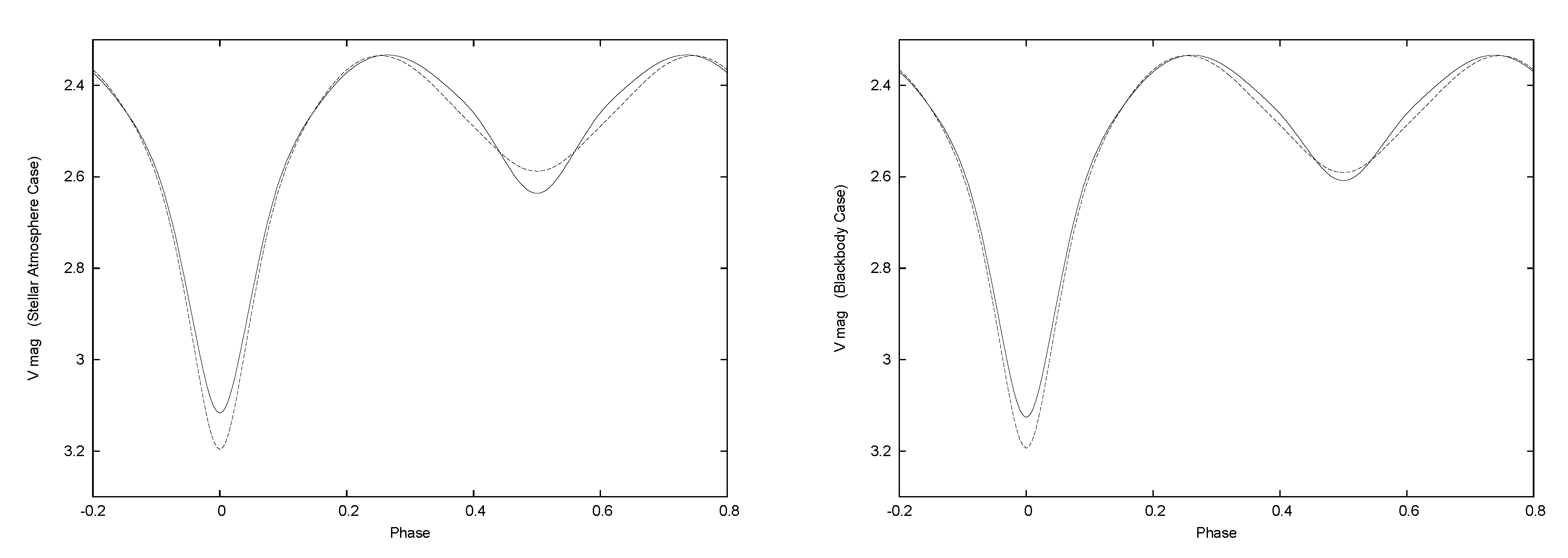
- However even assuming blackbody emission, thus avoiding stellar atmosphere irregularities, a measured light curve responds to and , not simply to their ratio, as shown by model computations. Figure 1 compares V band light curves for high and low temperature OC binaries (otherwise identical) with the same T-ratio. The panels show separate comparisons for stellar atmospheres and blackbodies. for both curves yet the curves obviously differ due to the actual temperatures differing, so no definite light curve corresponds to T-ratio 0.5.
- Consider now the inverse problem (solutions from light curves). With one temperature stepped over several fixed values and the other as output, a functional relation will be found, but no theorem predicts that it will be as simple as .
Some T-ratio contributions are intended for large surveys, for which temperature knowledge via spectra or color indices is lacking for most EBs. Since eclipse depth ratios give a rough indication of relative temperatures although not individual temperatures, T-ratios may be acceptably practical quantities to list in such circumstances. However statements are needed to tell how individual temperatures are set within the computations.
7.3. Parameter No-Nos
Some authors rig simultaneous solutions to favor a particular type of observation, contending that the number of velocity data points is small so the RV’s need help. Usually the help is given by arbitrary increases in RV weights. Analyses should not favor one dataset over another according to pre-set subjective notions.
Although traditional for many years, RV amplitudes (, ) are not proper parameters and never were, but are only descriptors of a plot. As an analogy, imagine that EB eclipse depths were to be given as light curve solution parameters. No one would accept that, as eclipse depths do not measure anything physical or geometric, being affected by a melange of phenomena, so they are certainly not system parameters. The ratio of Ks is sometimes regarded as measuring the ratio of absolute orbit sizes or the ratio of star masses, but it does that only for well-detached binaries. For tight binaries, is an approximation to mass and orbit size ratios, as it is affected by tides, irradiation, and other phenomena. The proper solution parameters are (absolute orbit sizes).
A referee commented that “sometimes authors include tables with the fitted parameters but not fixed ones (gravity brightening exponents, etc.). All fitted and fixed parameters should be listed so that absolute properties can be computed homogeneously”. I agree.
Third light () from sources other than the binary component stars (system member stars or non-members, circumstellar gas, CV nova shells, etc.) can be a rather common inclusion within binary system light curves. Analyses would be simpler and more accurate without this reality, but nature is not in the business of simplifying our lives. Anyway those extra sources can be very interesting in their own right, while other parameters are correlated with , and modern solution algorithms can deal with , so ignoring their possible presence is another no-no. Always check for third light.
8. Last Comment
Not everyone will agree with all the above items but perhaps each reader will agree with some, leading to reduced loss of observations, new explorations in modeling of CVs and other binaries with disks, further applications of morphological and other solution-related logic, and enhanced clarity of explanations.
Funding
This research received no external funding.
Acknowledgments
Josef Kallrath, Eugene Milone, Walter Van Hamme, and the referees made very good comments that improved the paper.
Conflicts of Interest
The author declares no conflicts of interest.
References
- Wilson, R.E. Invited Review Paper: Understanding Binary Stars Via Light Curves. IAPPP Commun. 1994, 55. [Google Scholar]
- Wilson, R.E. Binary star light-curve models. Astron. Soc. Pac. 1994, 106, 921–941. [Google Scholar] [CrossRef]
- Wilson, R.E.; Van Hamme, W.; Peters, G.J. Binary star analysis with intrinsic pulsation. Contrib. Astron. Obs. Skalnaté Pleso 2020, 50, 552–556. [Google Scholar] [CrossRef]
- Kuiper, G.P. Note on W Ursae Majoris Stars. Astrophys. J. 1948, 108, 541. [Google Scholar] [CrossRef]
- Mochnacki, S.W.; Doughty, N.A. A model for the totally eclipsing W Ursae Majoris system AW UMa. Mon. Not. R. Astron. Soc. 1972, 156, 51–65. [Google Scholar] [CrossRef]
- Mochnacki, S.W.; Doughty, N.A. Models for five W ursae majoris systems. Mon. Not. R. Astron. Soc. 1972, 156, 243–252. [Google Scholar] [CrossRef]
- Budaj, J. The Reflection Effect in Interacting Binaries or in Planet-Star Systems. Astron. J. 2011, 141, 59–70. [Google Scholar] [CrossRef]
- Prsa, A.; Conroy, K.E.; Horvat, M.; Pablo, H.; Kochoska, A.; Bloemen, S.; Giammarco, J.; Hambleton, K.M.; Degroote, P. Physics of eclipsing binaries. II. Toward the increased model fidelity. Astrophys. J. Suppl. Ser. 2016, 227, 29–48. [Google Scholar] [CrossRef]
- Kopal, Z. The classification of close binary systems. Ann. d’Ap 1955, 18, 370–430. [Google Scholar]
- Kopal, Z. Close Binary Systems; Chapman & Hall London: London, UK, 1959. [Google Scholar]
- Wilson, R.E. Eccentric orbit generalization and simultaneous solution of binary star light and velocity curves. Astrophys. J. 1979, 234, 1054–1066. [Google Scholar] [CrossRef]
- Zwicky, F. Morphological Astronomy; Springer-Verlag Publ.: Heidelberg, Germany, 1957; Chapter I. [Google Scholar]
- Wilson, R.E.; Devinney, E.J. Lobe overflow as the likely cause of pericenter outburst in an SMBH orbiter. Astrophys. J. 2015, 807, 80–83. [Google Scholar] [CrossRef]
- Wilson, R.E. Binary Star Morphology and the Name Overcontact. Inf. Bull. Var. Stars 2001, 5076, 1–3. [Google Scholar]
- Kallrath, J.; Milone, E.F. Eclipsing Binary Stars: Modeling and Analysis, 2nd ed.; Springer Publ.: New York, NY, USA, 2009; pp. 109–114, 238–241. [Google Scholar]
- Leung, K.C.; Sistero, R.F.; Zhai, D.; Grieco, A.; Candellero, B. Revised UBV photometric solution of the early-type contact system BH Centauri. Astron. J. 1984, 89, 872–875. [Google Scholar] [CrossRef]
- Bell, S.A.; Malcom, G.J. RZ Pyxidis: An early-type marginal contact binary. Mon. Not. R. Astron. Soc. 1987, 227, 481–500. [Google Scholar] [CrossRef][Green Version]
- Wilson, R.E.; Leung, K.C. V 701 Scorpii and its place among early contact binaries. Astron. Astrophys. 1977, 61, 137–140. [Google Scholar]
- Cakirli, O.; Ibanoglu, C.; Sipahi, E.; Fresca, A.; Catanzaro, G. Analysis of the massive eclipsing binary V1441 Aql. New Astron. 2015, 34, 15–20. [Google Scholar] [CrossRef]
- Linnell, A.P.; Harmanec, P.; Koubský, P.; Božić, H.; Yang, S.; Ruždjak, D.; Sudar, D.; Libich, J.; Eenens, P.; Krpata, J.; et al. Properties and nature of Be stars-24. Better data and model for the Be+ F binary V360 Lacertae. Astron. Astrophys. 2006, 455, 1037–1052. [Google Scholar] [CrossRef][Green Version]
- Palma, T.; Minniti, D.; Dekany, I.; Clariá, J.J.; Alonso-García, J.; Gramajo, L.; Alegría, S.R.; Bonatto, C. New variable stars discovered in the fields of three Galactic open clusters using the VVV survey. New Astron. 2016, 49, 50–62. [Google Scholar] [CrossRef]
- Terrell, D.; Nelson, R.H. The double contact nature of TT Herculis. Astrophys. J. 2014, 783, 35–40. [Google Scholar] [CrossRef]
- Wilson, R.E.; Van Hamme, W.; Pettera, L.E. RZ Scuti as a double contact binary. Astrophys. J. 1985, 289, 748–755. [Google Scholar] [CrossRef]
- Wilson, R.E. Eclipsing Binary Flux Units and the Distance Problem; Astronomical Society of the Pacific: San Francisco, CA, USA, 2007; Volume 362, pp. 3–14. [Google Scholar]
- Wilson, R.E. Eclipsing binary solutions in physical units and direct distance estimation. Astrophys. J. 2008, 672, 575–589. [Google Scholar] [CrossRef]
- Wilson, R.E.; Van Hamme, W.; Terrell, D. Flux calibrations from nearby eclipsing binaries and single stars. Astrophys. J. 2010, 723, 1469–1492. [Google Scholar] [CrossRef]
- Milone, E.F.; Schiller, S.J.; Mellergaard Amby, T.; Frandsen, S. DS Andromedae: A detached eclipsing double-lined spectroscopic binary in the galactic cluster NGC 752. Astron. J. 2019, 158, 82–117. [Google Scholar] [CrossRef]
- Bisikalo, D.V.; Harmanec, P.; Boyarchuk, A.A.; Kuznetsov, O.A.; Hadrava, P. Circumstellar structures in the eclipsing binary eta Lyr A. Gasdynamical modelling confronted with observations. Astron. Astrophys. 2000, 353, 1009–1015. [Google Scholar]
- Negueruela, I.; Okazaki, A.T. The Be/X-ray transient 4U 0115+ 63/V635 Cassiopeiae—I. A consistent model. Astron. Astrophys. 2001, 369, 108–116. [Google Scholar] [CrossRef]
- Okazaki, A.T.; Bate, M.R.; Ogilvie, G.I.; Pringle, J.E. Viscous effects on the interaction between the coplanar decretion disc and the neutron star in Be/X-ray binaries. Mon. Not. R. Astron. Soc. 2002, 337, 967–980. [Google Scholar] [CrossRef]
- Panoglou, D.; Faes, D.M.; Carciofi, A.C. Variability of the decretion disc of Be stars in binary systems. Rev. Mex. Astron. Astrofís. 2017, 49, 94. [Google Scholar]
- Terrell, D. Circumstellar Hydrodynamics and Spectral Radiation in Algols. 1994. Available online: http://ufdc.ufl.edu/AA00003229/00001 (accessed on 7 January 2019).
- Whitehurst, R. Numerical simulations of accretion discs—I. Superhumps: A tidal phenomenon of accretion discs. Mon. Not. R. Astron. Soc. 1988, 232, 35–51. [Google Scholar] [CrossRef]
- Whitehurst, R. Numerical simulations of accretion discs—II. Design and implementation of a new numerical method. Mon. Not. R. Astron. Soc. 1988, 233, 529–551. [Google Scholar] [CrossRef][Green Version]
- Wilson, R.E. Self-gravitating Semi-transparent Circumstellar Disks: An Analytic Model. Astrophys. J. 2018, 869, 19–36. [Google Scholar] [CrossRef]
- Abramowicz, M.A.; Curir, A.; Schwarzenberg-Czerny, A.; Wilson, R.E. Self-gravity and the global structure of accretion discs. Mon. Not. R. Astron. Soc. 1984, 208, 279–291. [Google Scholar] [CrossRef]
- Bodo, G.; Curir, A. Models of self-gravitating accretion disks. Astron. Astrophys. 1992, 253, 318–328. [Google Scholar]
- Fukue, J.; Sakamoto, C. Vertical structures of self-gravitating gaseous disks around a central object. Publ. Astron. Soc. Jpn. 1992, 44, 553–556. [Google Scholar]
- Hachisu, I. A versatile method for obtaining structures of rapidly rotating stars. Astrophys. J. Suppl. Ser. 1986, 61, 479–507. [Google Scholar] [CrossRef]
- Hachisu, I. A versatile method for obtaining structures of rapidly rotating stars. II—Three-dimensional self-consistent field method. Astrophys. J. Suppl. Ser. 1986, 62, 461–499. [Google Scholar] [CrossRef]
- Hachisu, I.; Kato, M.; Schaefer, B.E. Revised analysis of the supersoft X-ray phase, helium enrichment, and turnoff time in the 2000 outburst of the recurrent nova CI Aquilae. Astrophys. J. 2003, 584, 1008–1015. [Google Scholar] [CrossRef][Green Version]
- Hunter, J.H.; Wilson, R.E. A critical examination of thick disks with equatorial accretion. Astrophys. J. 1986, 302, 11–18. [Google Scholar] [CrossRef]
- Mineshige, S.; Umemura, M. Self-similar self-gravitating viscous disks. Astrophys. J. 1996, 469, L49–L51. [Google Scholar] [CrossRef]
- Paczynski, B.; Abramowicz, M.A. A model of a thick disk with equatorial accretion. Astrophys. J. 1982, 253, 897–907. [Google Scholar] [CrossRef]
- Wilson, R.E. Equilibrium figures for beta Lyrae type disks. Astrophys. J. 1981, 251, 246–258. [Google Scholar] [CrossRef]
- Wilson, R.E. Binary and Multiple Stars as Tracers of Stellar Evolution; Kopal, Z., Rahe, J., Eds.; Reidel Publ. Co.: Dordrecht, The Netherlands, 1982; pp. 261–273. [Google Scholar]
- Hachisu, I.; Kato, M. Prediction of the supersoft X-ray phase, helium enrichment, and turnoff time in the 2000 outburst of the recurrent nova CI aquilae. Astrophys. J. 2001, 553, L161–L164. [Google Scholar] [CrossRef]
- Klement, A.; Carciofi, A.C.; Rivinius, T.; Panoglou, D.; Vieira, R.G.; Bjorkman, J.E.; Štefl, S.; Tycner, C.; Faes, D.M.; Korčáková, D.; et al. Multitechnique testing of the viscous decretion disk model—I. The stable and tenuous disk of the late-type Be star β CMi. Astron. Astrophys. 2015, 584, A85. [Google Scholar] [CrossRef]
- Klement, R.; Carciofi, A.C.; Stefl, S.; Faes, D.M.; Rivinius, T. Detailed Modeling of β CMi: A Multi-Technique Test of the Viscous Decretion Disk Scenario. In Bright Emissaries: Be Stars as Messengers of Star-Disk Physics, Proceedings of a Meeting held at The University of Western Ontario, London, Ontario, Canada, 11–13 August 2014; Astronomical Society of the Pacific: San Francisco, CA, USA, 2016; Volume 506, p. 7. [Google Scholar]
- Kurfurst, P.; Feldmeier, A.; Krticka, J. Time-dependent modeling of extended thin decretion disks of critically rotating stars. Astron. Astrophys. 2014, 569, A23. [Google Scholar] [CrossRef]
- Lee, U. Viscous decretion discs around rapidly rotating stars. Publ. Astron. Soc. Jpn. 2013, 65, 2. [Google Scholar] [CrossRef]
- Wilson, R.E. An analytic self-gravitating disk model: Inferences and logical structure. Contrib. Astron. Obs. Skalnaté Pleso 2020, 50, 523–529. [Google Scholar]
- Huang, S. An Interpretation of Beta Lyrae. Astrophys. J. 1963, 138, 342–349. [Google Scholar] [CrossRef][Green Version]
- Wilson, R.E. The secondary component of Beta Lyrae. Astrophys. J. 1974, 189, 319–329. [Google Scholar] [CrossRef]
- Wilson, R.E.; Van Hamme, W. Unification of binary star ephemeris solutions. Astrophys. J. 2013, 780, 151–167. [Google Scholar] [CrossRef]
- Wilson, R.E. EB Light Curve Models—What’s Next? Astrophys. Space Sci. 2005, 296, 197–209. [Google Scholar] [CrossRef]
- Trimble, V. A field guide to the binary stars. Nature 1983, 303, 137–142. [Google Scholar] [CrossRef]
- McCarthy, M. Fr. Secchi and stellar spectra. Pop. Astron. 1950, 58, 153–168. [Google Scholar]
- Binnendijk, L. W Ursae Majoris Type Systems. J. R. Astron. Soc. Can. 1957, 51, 83–90. [Google Scholar]
- O’Connell, D.J.K. The so-called periastron effect in eclipsing binaries. Publ. Riverv. Coll. Obs. 1951, 2, 85–99. [Google Scholar] [CrossRef]
- O’Connell, D.J.K. The so-called periastron effect in eclipsing binaries. Mon. Not. R. Astron. Soc. 1951, 111, 642. [Google Scholar] [CrossRef]
| 1 | |
| 2 | A lobe-filling star’s surface is an equipotential set by loss of matter at a null point of effective gravity at periastron. |
| 3 | |
| 4 | Lower case designations d, c, and o are for binary components, while upper case designations D, SD, OC, and DBC are for binary systems. |
| 5 | A small subset of OC binaries, with temperatures too high to have convective envelopes, are not considered to be W UMas. They are uncommon objects, in contrast to the very abundant W UMas, and easily distinguished from them in several ways, including their early spectral types. Examples of these high temperature OC binaries are BH Centauri (see e.g., [16]), RZ Pyxidis (e.g., [17]), and V701 Scorpii (e.g., [18]). |
| 6 | No actual counts have been published, although that would be an interesting contribution, especially if the usage numbers were given versus time. |
| 7 | The author’s search to identify originators of those type name assignments did not succeed, although information on the three prototype systems is abundant. Presumably any new investigation into the relevant history can safely begin at the mid 1940s, when photomultiplier photometry began producing many good light curves. |
| 8 | Algols having very unequal primary and secondary eclipse depths, W UMa depths being nearly equal, and Lyrs being intermediate in that regard. |
| 9 | See McCarthy [58] for history, including contributions leading up to the types by Angelo Secchi. |
| 10 | The subtypes of W UMas were originally defined [59] according to whether the slightly deeper eclipse is that of the larger or smaller star (respectively A and W type). |
| 11 | An efficient scheme to solve such problems is that of Lagrange multipliers. |
| 12 | Presumably corresponding to suitably weighted surface means of and . |
Figure 1.
Left panel: V band light curves for model OC binaries of high [16,000; 8000] K (continuous line) and low [8000; 4000] K (dashed line) temperature. All other parameters are the same for the two curves, with limb darkening computed from local physical variables and aspect. The vertical shift between curves is set so that they agree at phase 0.25, since few published light curves are in absolute physical units. for both curves yet they obviously differ, so no definite light curve corresponds to T-ratio 0.5. Right panel: resulting curves for blackbody emission with all input quantities the same as for the left panel. The high and low T blackbody curves differ but are somewhat closer than the atmosphere curves.

© 2020 by the author. Licensee MDPI, Basel, Switzerland. This article is an open access article distributed under the terms and conditions of the Creative Commons Attribution (CC BY) license (http://creativecommons.org/licenses/by/4.0/).
Share and Cite
MDPI and ACS Style
Wilson, R.E. Close Binary Perspectives. Galaxies 2020, 8, 57. https://doi.org/10.3390/galaxies8030057
AMA Style
Wilson RE. Close Binary Perspectives. Galaxies. 2020; 8(3):57. https://doi.org/10.3390/galaxies8030057
Chicago/Turabian StyleWilson, R.E. 2020. "Close Binary Perspectives" Galaxies 8, no. 3: 57. https://doi.org/10.3390/galaxies8030057
APA StyleWilson, R. E. (2020). Close Binary Perspectives. Galaxies, 8(3), 57. https://doi.org/10.3390/galaxies8030057
Note that from the first issue of 2016, this journal uses article numbers instead of page numbers. See further details here.