Abstract
Circular polarization (CP) provides an invaluable probe into the underlying plasma content of relativistic jets. CP can be generated within the jet through a physical process known as linear birefringence. This is a physical mechanism through which initially linearly polarized emission produced in one region of the jet is attenuated by Faraday rotation as it passes through other regions of the jet with distinct magnetic field orientations. Marscher developed the turbulent extreme multi-zone (TEMZ) model of blazar emission which mimics these types of magnetic geometries with collections of thousands of plasma cells passing through a standing conical shock. I have recently developed a radiative transfer algorithm to generate synthetic images of the time-dependent circularly polarized intensity emanating from the TEMZ model at different radio frequencies. In this study, we produce synthetic multi-epoch observations that highlight the temporal variability in the circular polarization produced by the TEMZ model. We also explore the effect that different plasma compositions within the jet have on the resultant levels of CP.
1. Introduction
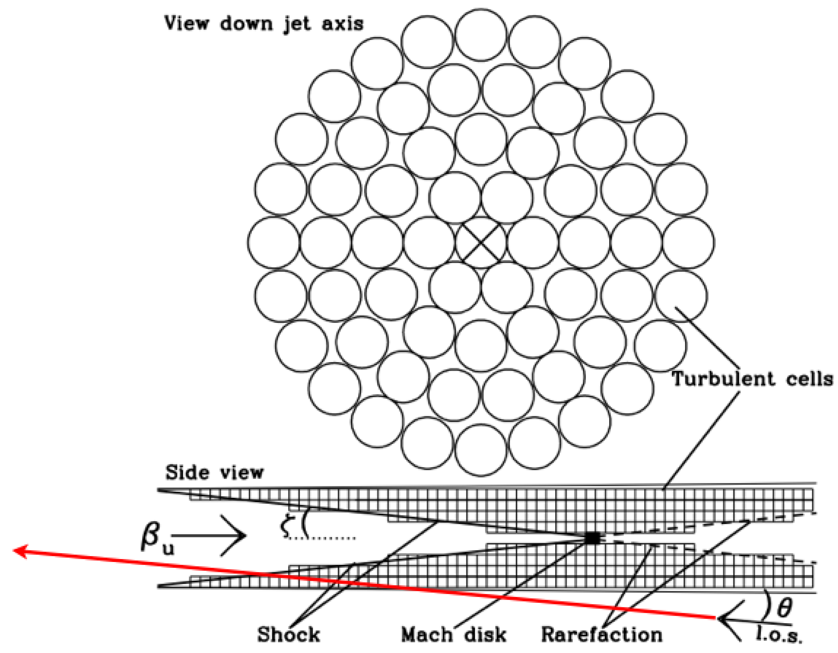
Circularly polarized emission (Stokes V) has been observed in the radio cores of a number of blazars [1]. This form of polarization can potentially be used as a probe of the plasma content of the jet [2]. However, circular polarization (CP) emission is notoriously very faint (<1 % of Stokes I) and difficult to calibrate. The dominant physical mechanism driving the production of CP in blazars is believed to be a birefringent effect known as Faraday conversion, in which varying magnetic field orientations within the jet convert initially linearly polarized emission into circular polarization. In order to better understand the variability seen in the polarized emission from blazars, Marscher (2014) [3] created the turbulent extreme multi-zone (TEMZ) model for blazar emission. This emission model is made up of thousands of individual cells of plasma that move relativistically across a stationary conical shock (Figure 1). Plasma cells within the model are randomly assigned a magnetic field strength (and orientation) that consists of (i) a turbulent component and (ii) a vector-ordered component. The combined emission from the TEMZ cells is able to reproduce much of the variability that is observed in the linearly polarized emission from blazars [3]. The TEMZ model naturally creates a birefringent plasma through which circularly polarized emission can be generated via Faraday conversion [4]. In this paper, we extend our modeling efforts in order to study the temporal variability of CP produced by the TEMZ model (see Section 4) and to explore how sensitive CP is to the underlying plasma content of the jet (see Section 5).
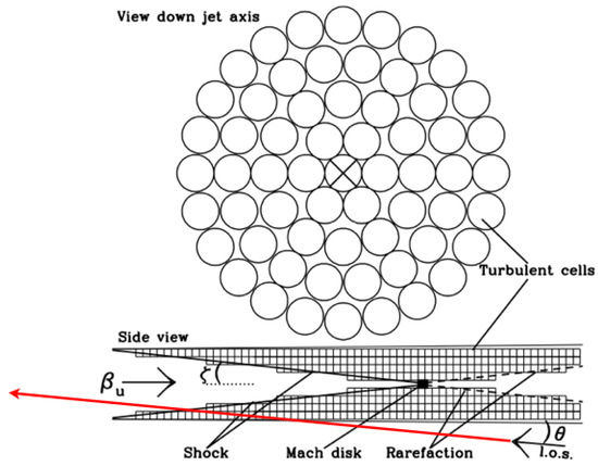
Figure 1.
A depiction of the turbulent extreme multi-zone (TEMZ) model—reproduced by permission from [3]. The emission from the radio core of a blazar is modeled as the aggregate emission emanating from thousands of turbulent cells of plasma moving relativistically across a conical shock. The red line illustrates that along a given line-of-sight through the TEMZ model, a ray will cross multiple cells of plasma with varying magnetic field orientations.
2. The Full Stokes Equations
I have written a numerical algorithm to solve the full Stokes equations of polarized radiative transfer (outlined in [5,6]). My code solves the following matrix along sight-lines passing through the TEMZ model:
where , , , and are the frequency-dependent Stokes parameters. The terms and are frequency-dependent emission and absorption coefficients for each of the four Stokes parameters. The Faraday effects of rotation and conversion are included in the and terms, respectively. Optical depth effects are also included, and the path length through each plasma cell is given by l. Equation 1 has an analytic solution that is presented in [5]. I apply this analytic solution along each ray (highlighted by the red line in Figure 1), tracking the polarized radiative transfer through the various computational cells encountered by each ray. I have incorporated my polarized radiative transfer scheme into the ray-tracing code RADMC-3D (see http://ascl.net/1202.015). This code creates synthetic images of the polarized emission produced by the TEMZ model by casting thousands of rays to build up the emission from the entire model.
3. Order and Disorder: Turbulence in the Jet
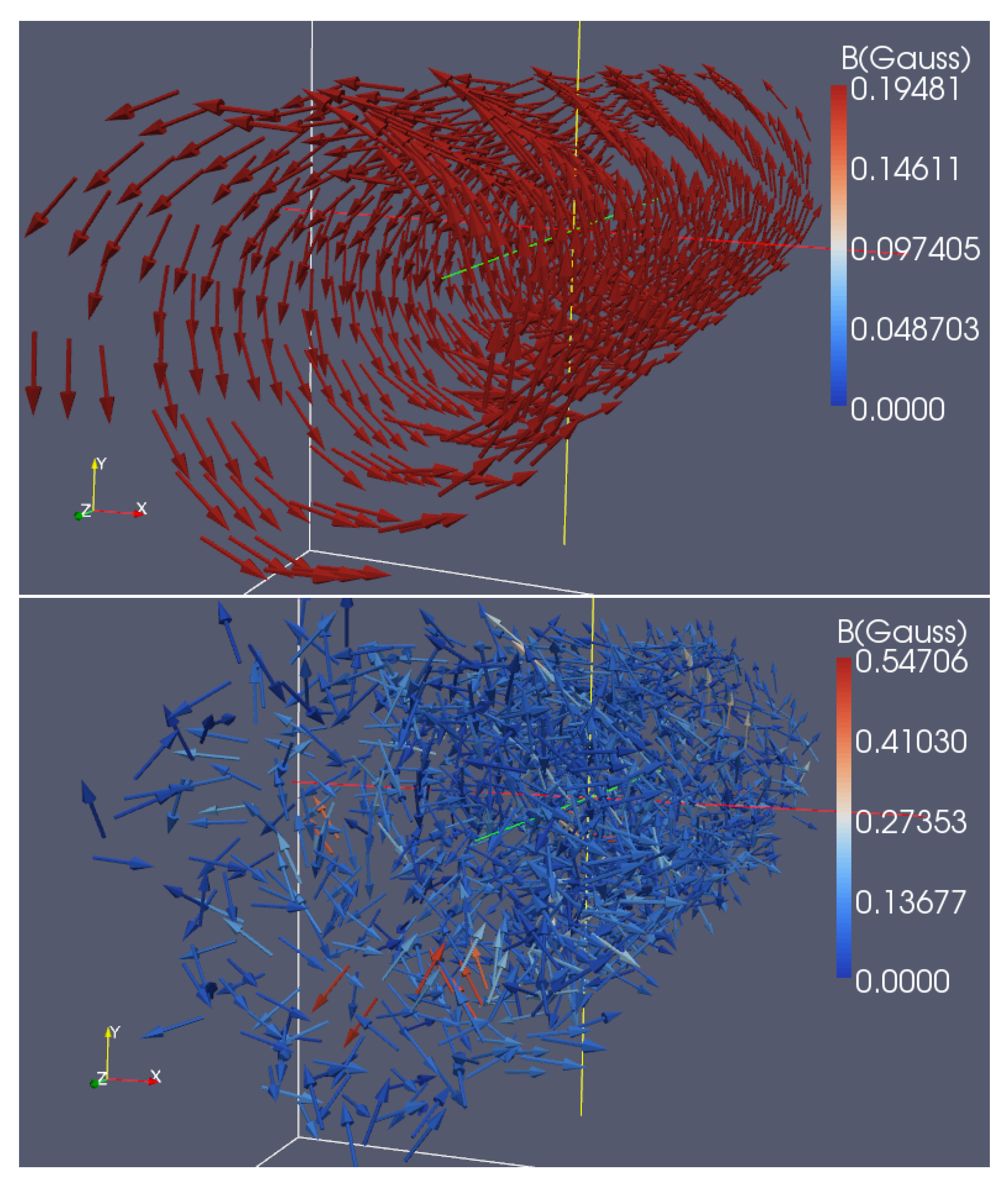
The turbulent nature of the jet is a free parameter within the TEMZ model. In order to explore the effect that turbulence (and its associated birefringence) has on the level of CP produced by the TEMZ model, I performed ray-tracing calculations through (i) an ordered helical magnetic field, and (ii) a disordered turbulent magnetic field (shown in the upper and lower panels of Figure 2, respectively). The turbulent field follows a Kolmogorov spectrum, with each cell having a distinct turbulent field component that is correlated with the magnetic fields of neighboring cells. The TEMZ computational grid is made up of individual plasma cells organized into seven concentric cylindrical shells that create the conical shock shown in Figure 1. For the ray-tracing calculations presented in this paper, the TEMZ cells were mapped onto rectilinear cartesian grids through which the polarized radiative transfer was performed. The sizes of the rectilinear grids were chosen based on the outermost TEMZ cylinder, which is 112 cells in length. RADMC-3D cast individual rays creating pixel images of the resultant polarized emission from each model (presented in [4]). The angle of inclination of the jet to our line-of-sight was fixed to for each of the calculations, and the jet plasma was given a bulk Lorentz factor of . The time-step of the code is set to the time it takes the turbulent plasma to propagate through the plasma cells, which each have a characteristic length of pc. The TEMZ model introduces variations in the particle energy density of the jet plasma upstream of the shock. The turbulent plasma then flows through the TEMZ grid and crosses the standing conical shock. Upon crossing the shock, the electrons are subjected to effects of radiative cooling. After initializing both the ordered and disordered TEMZ models, we ran both simulations forward in time, tracking the polarized emission from one time-step to the next.
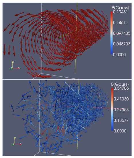
Figure 2.
(Upper panel) A 3D visualization of the ordered helical magnetic field within the first TEMZ simulation. Each vector highlights the magnetic field strength within an individual plasma cell (see color bar to the right for field strength in Gauss). (Lower panel) A 3D visualization of the disordered magnetic field within the second TEMZ simulation. The field here is partially re-ordered after crossing the conical shock.
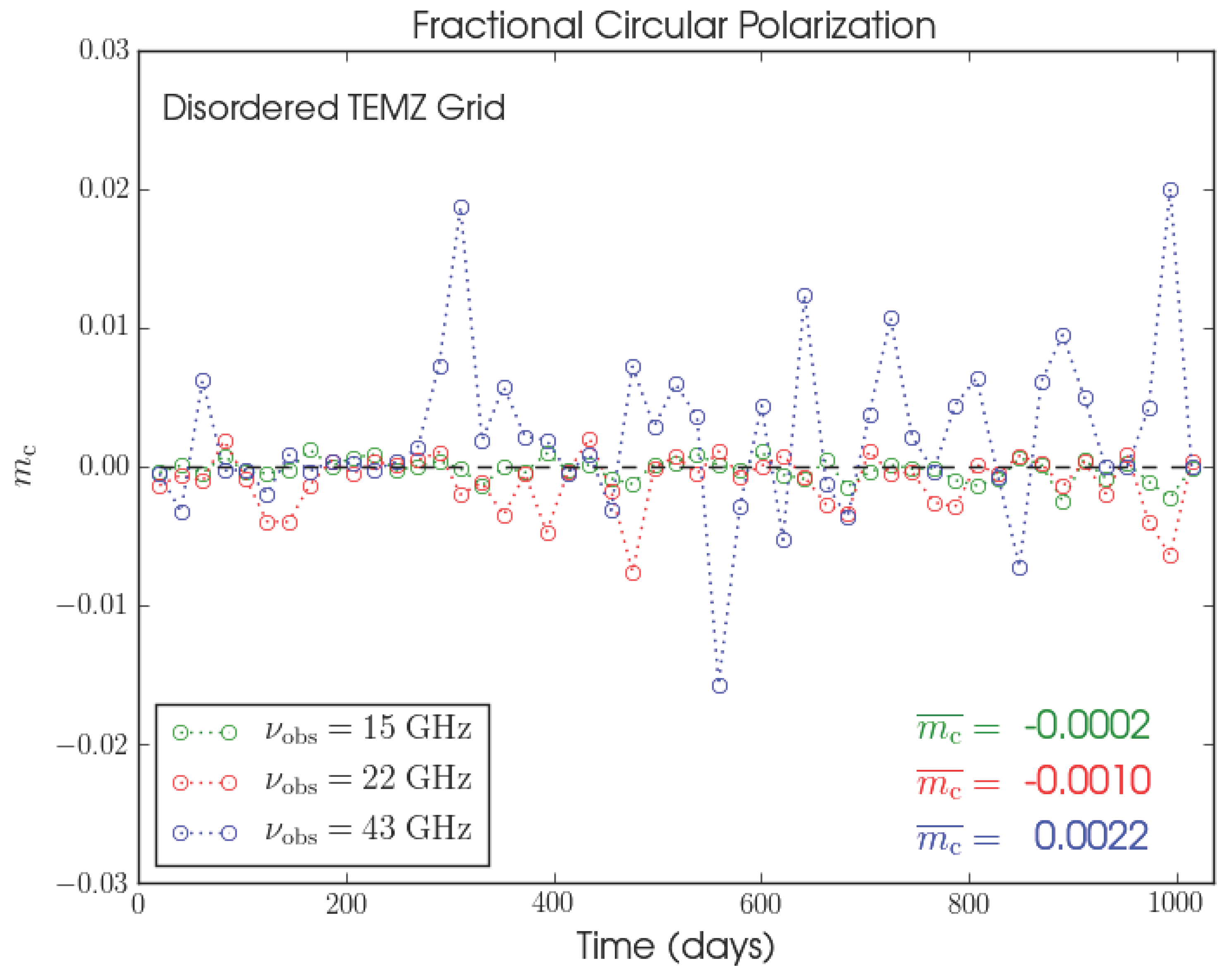
4. Temporal Variability of Circular Polarization
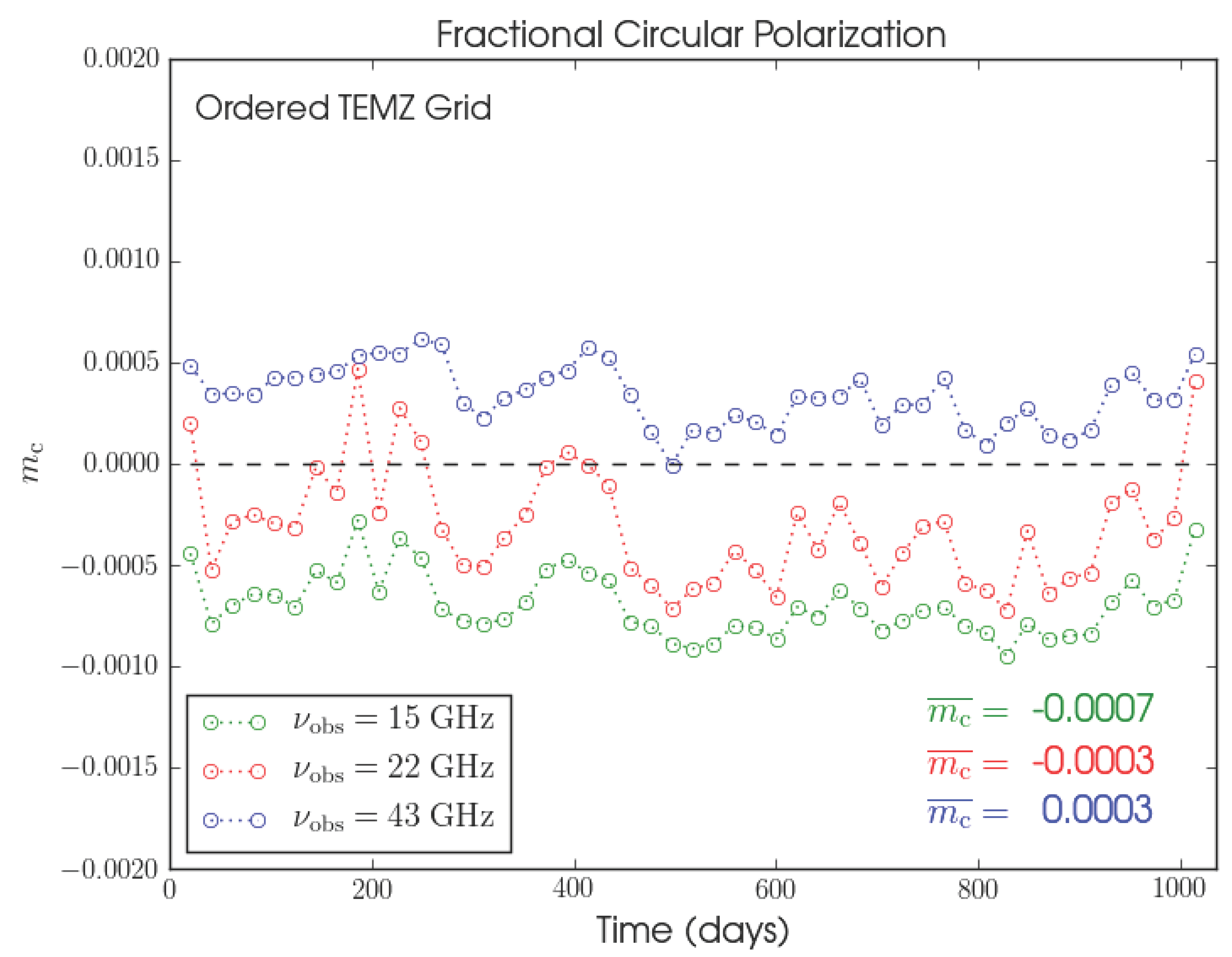
There have been several observational programs dedicated to monitoring the temporal variability of CP emanating from blazars (e.g., [7,8]). An interesting discovery was the occurrence of sudden reversals in the sign of the observed fractional circular polarization () in a number of blazars (i.e., flipping between +0.01 and −0.01). It was suggested that these reversals in sign may be related to turbulent magnetic fields within the radio cores of these jets [8]. There are, however, other sources which exhibit remarkable stability in the sign of , perhaps demonstrating a form of magnetic memory. Enßlin [9] postulated that in these sources Faraday conversion occurs as the jet emission passes through a twisted/helical magnetic field rather than a turbulent magnetic field. In order to investigate these two physical scenarios, we have carried out a time series analysis of the integrated levels of produced by the TEMZ model using the two different magnetic field grids depicted in Figure 2. We monitored the integrated levels of the fractional circular polarization for each model. The results are shown in Figure 3 at frequencies of 15, 22, and 43 GHz. The sign of remains fairly constant in the ordered field case (upper panel), in keeping with the prediction of [9]. In contrast, when the field is disordered, we see successive increases and decreases in the sign of , which perhaps mimic, to some extent, the reversals seen by [8] (lower panel). We also point out that in the ordered field case (upper panel) the three curves appear to have very similar shapes with systematic offsets that increase with frequency. We plan on comparing this type of ordered field behavior to temporal multi-frequency CP measurements of sources from the F-GAMMA program (http://www3.mpifr-bonn.mpg.de/div/vlbi/fgamma/fgamma.html).
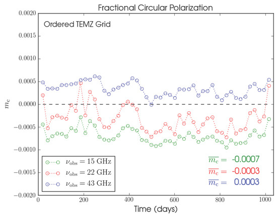
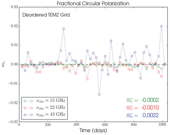
Figure 3.
(Upper panel) Variations of mc for the ordered field case (see Figure 2, upper panel). The green, red, and blue points correspond to observations at νobs = 15, 22, and 43 GHz, respectively. The average values of mc for each frequency over the length of the runs are listed in the lower right corner. (Lower panel) Corresponding variability in mc for the disordered field case (see Figure 2, lower panel).
5. Probing the Plasma Content of the Jet
The plasma composition of relativistic jets remains an active area of research. To parameterize this unknown composition in our TEMZ ray-tracing calculations, we included the following term in our synchrotron emissivities:
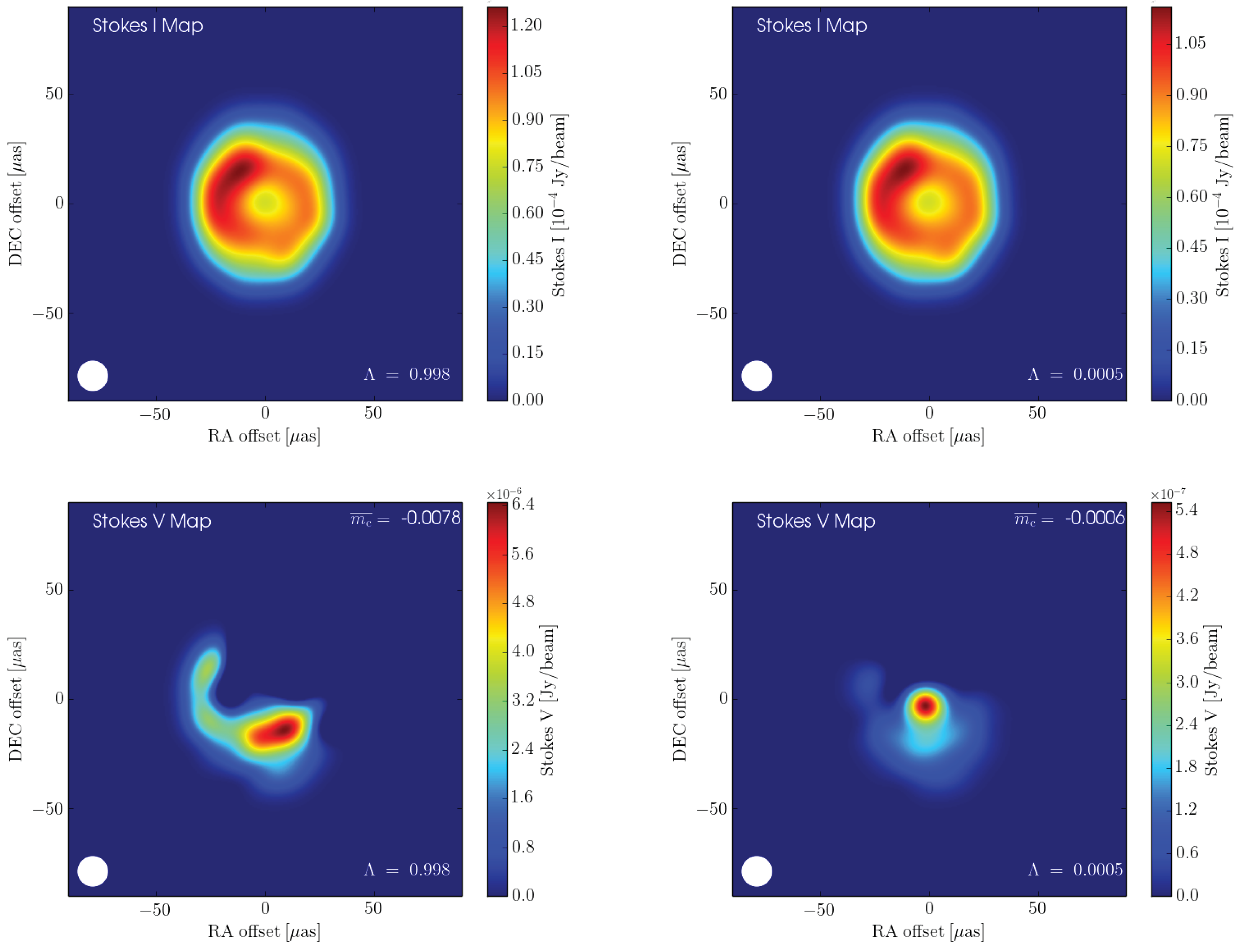
where are the number densities of the electrons/positrons, respectively [10]. Assuming the jet is electrically neutral, it then follows that the number density of protons is: . Equation 2 also assumes that the magnetic field within each plasma cell is uniform in nature. A pure electron–proton plasma within the jet would correspond to . We investigate here the effect that adding a positron content to the jet has on our TEMZ images for the turbulent field case (Figure 2, lower panel). We ran two ray-tracing calculations: one for a “normal” plasma consisting of a proton-to-positron ratio of 1000 (), while the second calculation consisted of a pair plasma with a proton-to-positron ratio of 0.001 (). Figure 4 presents a comparison of the resultant emission from the turbulent TEMZ model for these two plasma compositions. The differences in the Stokes V images (lower panels) highlights the sensitivity of CP to the underlying plasma content of the jet. We also note that the integrated level of fractional circular polarization () is an order of magnitude higher for the normal plasma in comparison to the pair plasma.
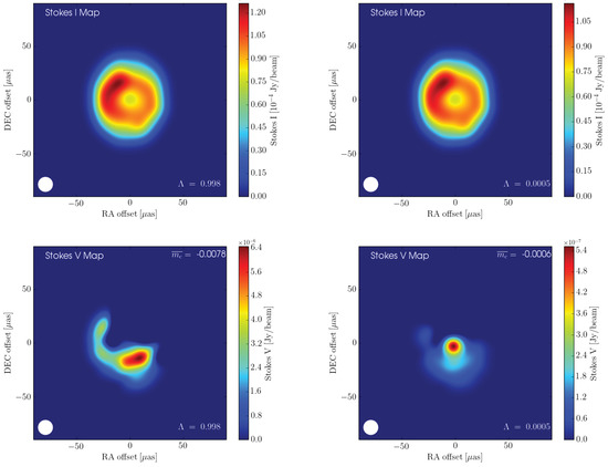
Figure 4.
(Upper left panel) Stokes I image for a jet composed of a normal plasma with a proton-to-positron ratio of 1000 (). (Upper right panel) Stokes I image for a jet composed of a pair plasma with a proton-to-positron ratio of 0.001 (). (Lower left panel) Corresponding Stokes V image for the normal plasma. (Lower right panel) Corresponding Stokes V image for the pair plasma. The above images have all been convolved with the circular Gaussian beam (shown in the lower left of each image), and were all created from the disordered TEMZ model (Figure 2, lower panel) at 43 GHz. The integrated level of fractional circular polarization () is listed in the upper right of the Stokes V images. For ease of visualization, we have masked the negative Stokes V values.
6. Future Research
We plan on carrying out a full parameter survey to investigate what other changes in the TEMZ model parameters create noticeable effects in the level (and variability) of circular polarization produced by the model. This survey will be useful in assessing how sensitive circular polarization is to the other physical conditions within the jet. We point out that our radiative transfer code can easily be applied to modeling other types of active galactic nuclei (i.e., by varying the angle of inclination of the jet). I am currently involved in an effort to model the radio emission/spectrum of the radio galaxy 3C 84. I have also begun to use my polarized radiative transfer algorithm to ray-trace through other types of numerical jet simulations (e.g., kinetic particle-in-cell calculations).
Conflicts of Interest
The authors declare no conflict of interest.
References
- Homan, D.C.; Lister, M.L.; Aller, H.D.; Aller, M.F.; Wardle, J.F.C. Full polarization spectra of 3C 279. Astrophys. J. 2009, 696. [Google Scholar] [CrossRef]
- Homan, D.C.; Attridge, J.M.; Wardle, J.F.C. Parsec-scale circular polarization observations of 40 blazars. Astrophys. J. 2001, 556. [Google Scholar] [CrossRef]
- Marscher, A.P. Turbulent, extreme multi-zone model for simulating flux and polarization variability in blazars. Astrophys. J. 2014, 780. [Google Scholar] [CrossRef]
- Macdonald, N.R. Through the Looking Glass: Faraday Conversion in Turbulent Blazar Jets. Galaxies 2016, 4. [Google Scholar] [CrossRef]
- Jones, T.W.; O’Dell, S.L. Transfer of polarized radiation in self-absorbed synchrotron sources. I. Results for a homogeneous source. Astrophys. J. 1977, 214, 522–539. [Google Scholar] [CrossRef]
- Jones, T.W. Polarization as a probe of magnetic field and plasma properties of compact radio sources- Simulation of relativistic jets. Astrophys. J. 1988, 332, 678–695. [Google Scholar] [CrossRef]
- Aller, M.F.; Aller, H.D.; Hughes, P.A. Radio Band Observations of Blazar Variability. J. Astrophys. Astron. 2011, 32. [Google Scholar] [CrossRef]
- Aller, H.D.; Aller, M.F.; Plotkin, R.M. Circular Polarization Variability in Extragalactic Sources on Time Scales of Months to Decades. Astrophys. Space Sci. 2003, 288, 17–28. [Google Scholar] [CrossRef]
- Enßlin, T.A. Does circular polarisation reveal the rotation of quasar engines? Astron. Astrophys. 2003, 401, 499–504. [Google Scholar] [CrossRef]
- Wardle, J.F.C.; Homan, D.C. Theoretical Models for Producing Circularly Polarized Radiation in Extragalactic Radio Sources. Astrophys. Space Sci. 2003, 288, 143–153. [Google Scholar] [CrossRef]
© 2017 by the author. Licensee MDPI, Basel, Switzerland. This article is an open access article distributed under the terms and conditions of the Creative Commons Attribution (CC BY) license (http://creativecommons.org/licenses/by/4.0/).