1. Introduction
Dwarf galaxies of the Local Group [
1,
2] comprise a unique laboratory for testing current theories of structure formation and evolution in the Universe at small scales. Until recently, their properties were believed to be a source of a number of problems for the formation theory based on cold dark matter. The problems included their insufficient number in the Local Group (the problem of missing satellites) and their reportedly flat inner dark matter profiles, contrary to predictions (the cusp/core problem). It seems, however, that the main origin of these problems can be traced to simplifications inherent in using simulations based on dark matter only and neglecting the effect of baryons on the structure and evolution of dwarfs.
The inclusion of baryonic physics in new, more advanced simulations demonstrated that baryons matter even in such dark matter dominated objects as the dwarf spheroidal (dSph) galaxies of the Local Group. It has been shown that the supernova feedback is able to blow out a sufficient amount of mass from the dwarf galaxy center in order to modify the inner distribution of dark matter [
3,
4]. If the process occurred early enough, this could have an effect on the subsequent evolution of the dwarfs in the vicinity of larger galaxies such as the Milky Way or M31. One of the key mechanisms responsible for the creation of the present-day population of dwarf galaxies around us is believed to be related to tidal forces from the host galaxies [
5]. According to such scenarios, the dwarfs, originally in the form of dwarf irregular galaxies, were accreted by bigger hosts at redshift
–2 and later stripped and stirred by tidal forces.
The details of the process depend on the structural parameters of the dwarfs and their orbits, but rely critically on the inner dark matter distribution in the dwarfs. If their dark matter profiles are cuspy, as predicted by dark matter-only simulations, they turn out to be very resilient to tides and can survive even on very tight orbits [
6,
7] in spite of losing a substantial fraction of mass and transforming into pressure- rather that rotation-supported systems. However, if their dark matter profiles were flattened prior to tidal evolution, they will be much more affected by tidal forces which, for tight enough orbits, may lead to their complete disruption [
8,
9,
10]. This will obviously result in reducing the population of dwarfs and thus solve the missing satellites problem [
11].
Here, we present and discuss, in detail, an illustrative example of the evolution of a disky dwarf galaxy in such a scenario. We assume that the dwarf’s inner dark matter profile has been flattened as a result of evolution in isolation. We place such a dwarf on a rather tight, but typical orbit around the Milky Way. We demonstrate that it indeed is completely dissolved after about 3 Gyr of evolution. We discuss the properties of the dwarf prior to and at the time of disruption. We also point out difficulties in distinguishing such a dissolving dwarf from similar-looking but still bound configurations and comment on the related problems involved in studying such dwarfs and inferring their dark matter content.
2. Methods
We have run an
N-body simulation of a dwarf galaxy orbiting a Milky Way-like host. The initial conditions for the simulation consisted of
N-body realizations of the two galaxies generated via procedures provided by L. Widrow [
12,
13]. Both galaxies contained exponential disks embedded in dark matter haloes with profiles similar to Navarro-Frenk-White (NFW) ones [
14], each made of
particles (
total). The simulation setup was similar to those in [
15,
16] except that the dwarf galaxy progenitor had a shallower dark matter profile. Specifically, its initial dark matter distribution was given by
, where
is the scale radius, with an asymptotic inner radial dependence
and an outer one
. We adopted the inner slope
, in agreement with the range of values following from cosmological simulations of dwarf galaxy formation in isolation [
3]. The total dark halo mass of the dwarf, after cut-off at the virial radius, was
M
. Its disk had a mass
M
, an exponential scale-length
kpc and thickness
. Our choice of these parameters is motivated by the typical dark mass of surviving subhaloes in simulated Local Group-like environments, the low efficiency of star formation in dwarfs and their larger thickness in comparison with normal-size galaxies. A thorough discussion on the justification of these choices can be found in [
6].
The host galaxy was similar to the model MWb of [
12]. It had a standard NFW cuspy dark matter halo (with inner slope of
), the total mass
M
and concentration
. The disk of the host had a mass
M
, the scale-length
kpc and thickness
kpc. The disk of the Milky Way was coplanar with the orbit of the dwarf. The dwarf galaxy was initially placed at an apocenter of a rather tight, eccentric orbit around the Milky Way with an apo- to pericenter distance ratio of
kpc. The eccentricity of the orbit is typical for subhaloes in simulated Milky Way-like environments [
17] and its size is similar to that of Carina, one of the classical dSph satellites of the Milky Way [
18]. The initial position was at the coordinates
kpc of the simulation box and the velocity vector of the dwarf was toward the negative
Y direction. The orientation of the dwarf galaxy disk was exactly coplanar with the orbit and prograde which ensures the strongest resonant effect of tidal forces [
16].
The evolution of the simulated system was followed for 5 Gyr using the GADGET-2
N-body code [
19,
20] with outputs saved every 0.05 Gyr. The adopted softening scales were
kpc and
kpc for the disk and halo of the dwarf while
kpc and
kpc for the disk and halo of the host, respectively.
3. Results
For the adopted orbit, the first pericenter passage occurs after
Gyr of evolution and the second after
Gyr. The analysis of the simulation outputs reveals that the dwarf galaxy survives the first pericenter but is disrupted after the second.
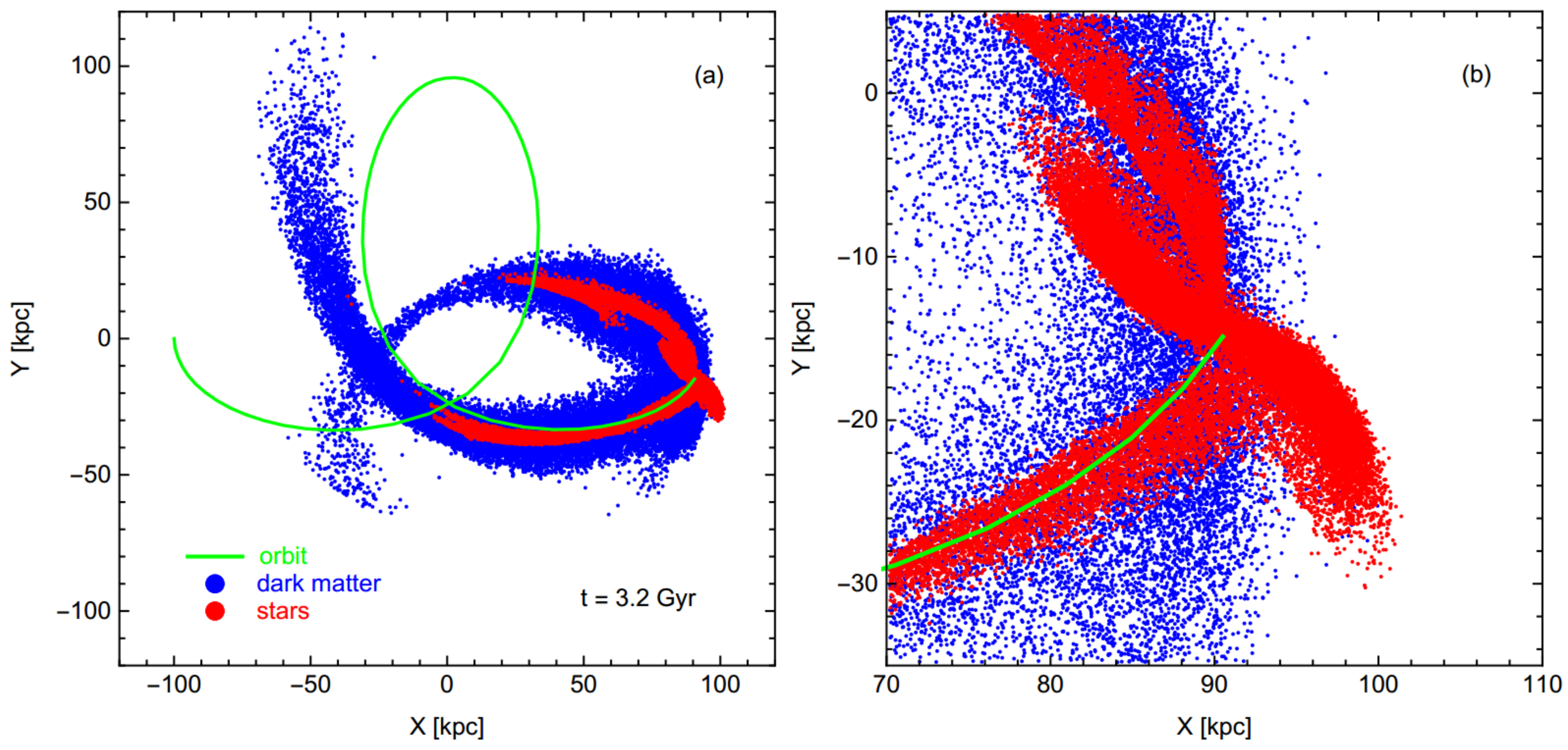
Figure 1 presents the distribution of stars and dark matter originating from the dwarf at
Gyr after the start of the simulation. The left panel of the Figure shows the general view of the two components in projection onto the orbital plane. The dark matter is shown in blue and the stars in red, while the orbit followed by the dwarf up to this time is drawn with a green line. Both components possess extended tidal tails, but as expected due to their different initial distributions, the tidal tails formed by dark matter are wider and longer. The right panel displays a closer view of the dwarf at the same time. The plot clearly shows the inner, shorter tidal tails formed in the last (second) pericenter passage on top of the longer ones produced earlier. Note that the inner tails are aligned more with the direction towards the host, while the older debris follows the orbit [
21,
22].
The time of
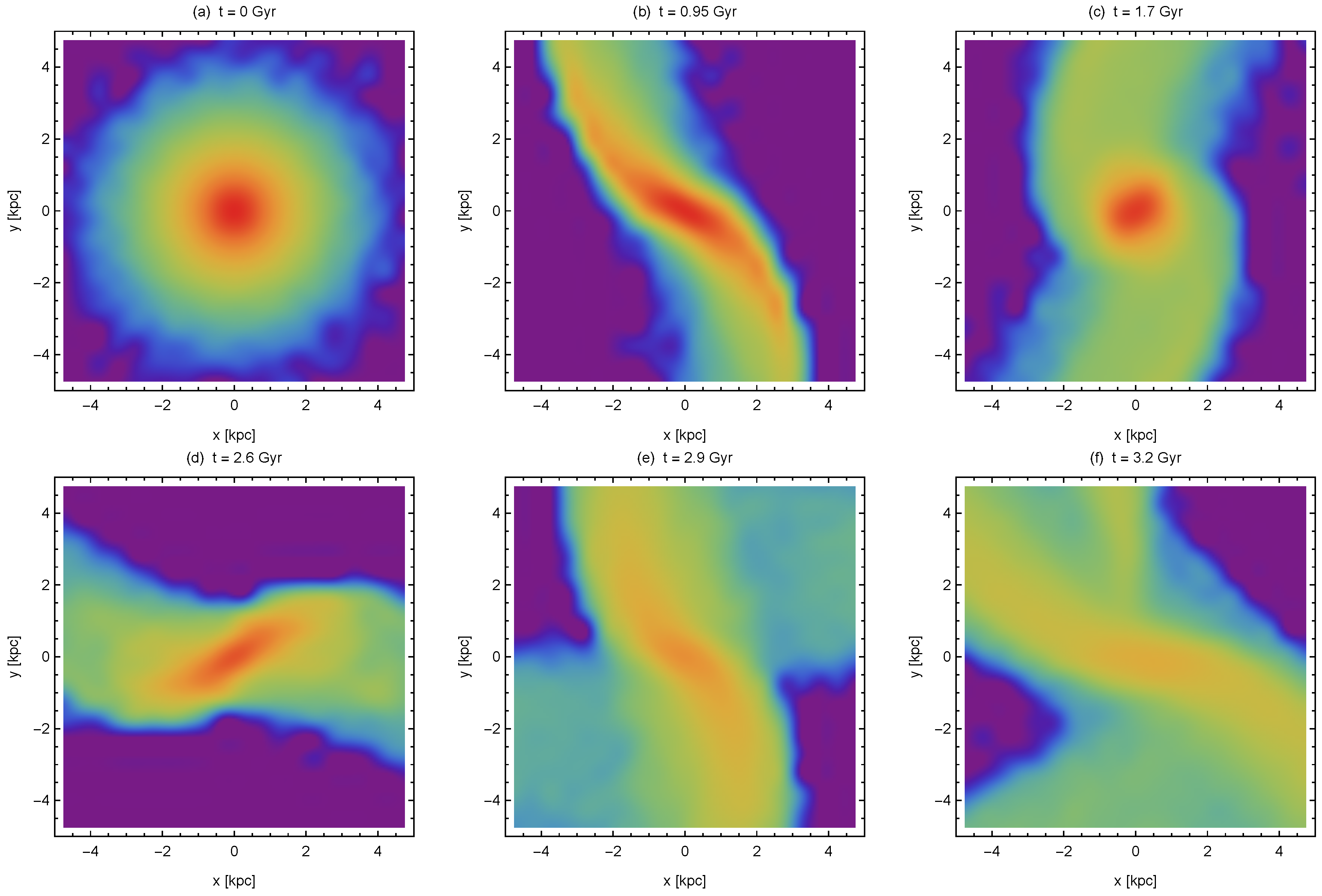
Gyr can be considered as the time of disruption since at this point and afterwards the density profile of the stellar component is so flat and the mass content in the central part so low (see below) that the center and properties of the dwarf cannot be reliably determined. The process of disruption is illustrated in
Figure 2 where we show the surface density distribution of the stars in the dwarf at different epochs in projection onto the orbital plane (which is also the plane of the dwarf’s disk). The three upper panels (from the left to the right) correspond to the initial configuration (
Gyr), the one just after the first pericenter passage (
Gyr) and to the second apocenter (
Gyr). At the beginning, the stellar distribution is obviously disky and regular, and at the first pericenter, it is strongly deformed and elongated. Following the strong stripping at the first pericenter, the dwarf in the third panel is much less extended and surrounded by the tidally stripped material but retains a compact, circular shape in projection. On the other hand, after the second pericenter (the three lower panels of
Figure 2), the dwarf gets elongated again but never recovers this compact circular shape and disrupts completely. The lower right panel of the Figure shows the surface density distribution of the stars at the time of disruption,
Gyr, the same as in
Figure 1.
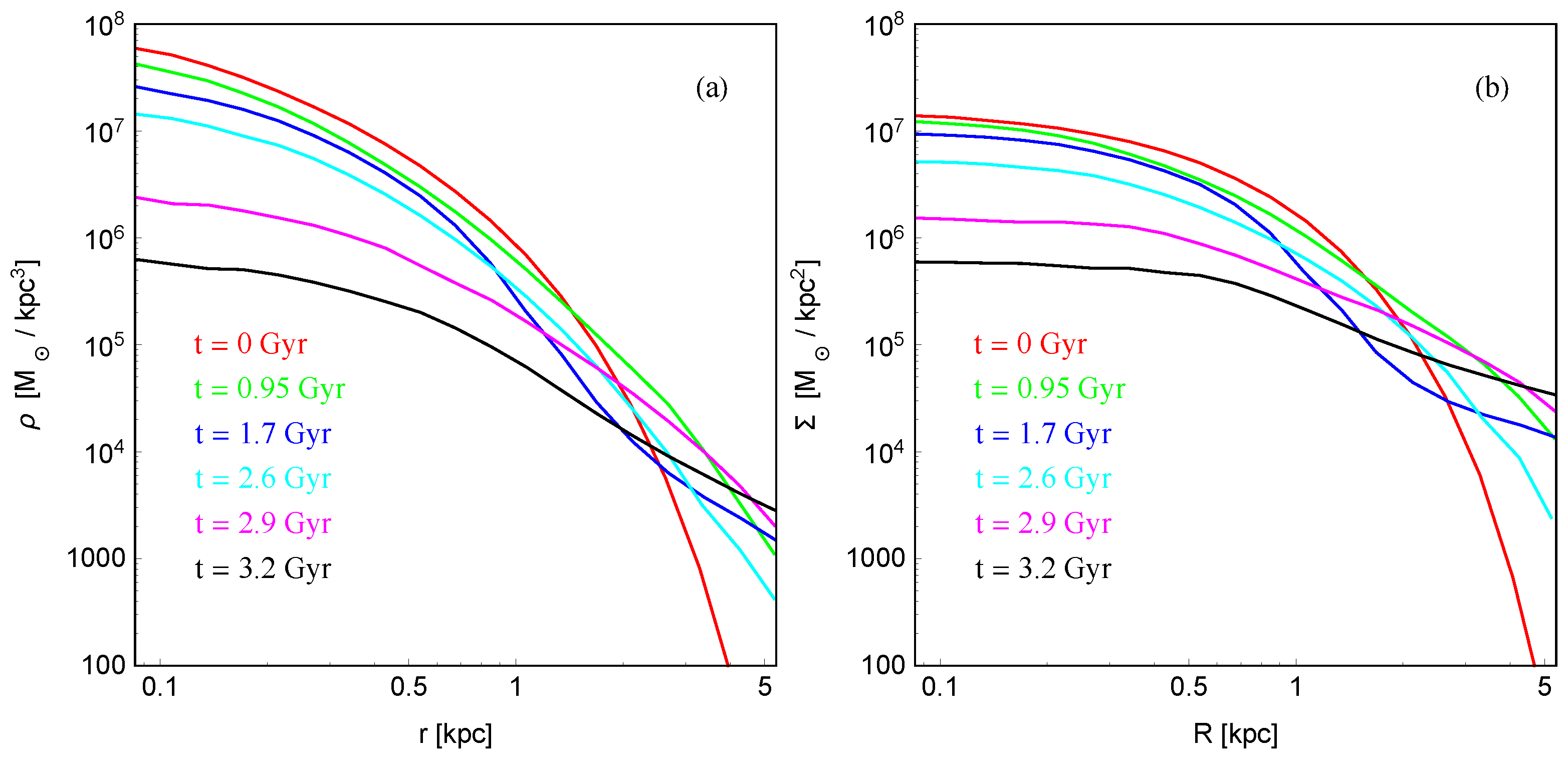
Figure 3 describes the dissolution of the dwarf in terms of the profiles of the stellar component measured as a function of a 3D radius
r (left panel) and as a function of the projected radius
R in the orbital plane (right panel). The examples of the profiles shown with different colors correspond to the same outputs as shown in
Figure 2, starting from the initial one at
Gyr, when the dwarf is an exponential disk, until
Gyr, when the dwarf dissolves. At the latter time, the density profiles are so shallow that the center of the dwarf cannot be reliably determined any more. Since the disruption occurs mainly in the orbital plane, the projected profiles are much shallower. We note that, contrary to the common misconception, tidal stripping leads to a dramatic decrease of the density also (or even mostly) in the inner part of the dwarf. The outer parts instead are populated by stars stripped from the dwarf and forming tidal tails. The power-law density distribution in the tails is especially well visible at the second apocenter at
Gyr [
22], although the density in the outskirts is higher than the initial one for all outputs shown.
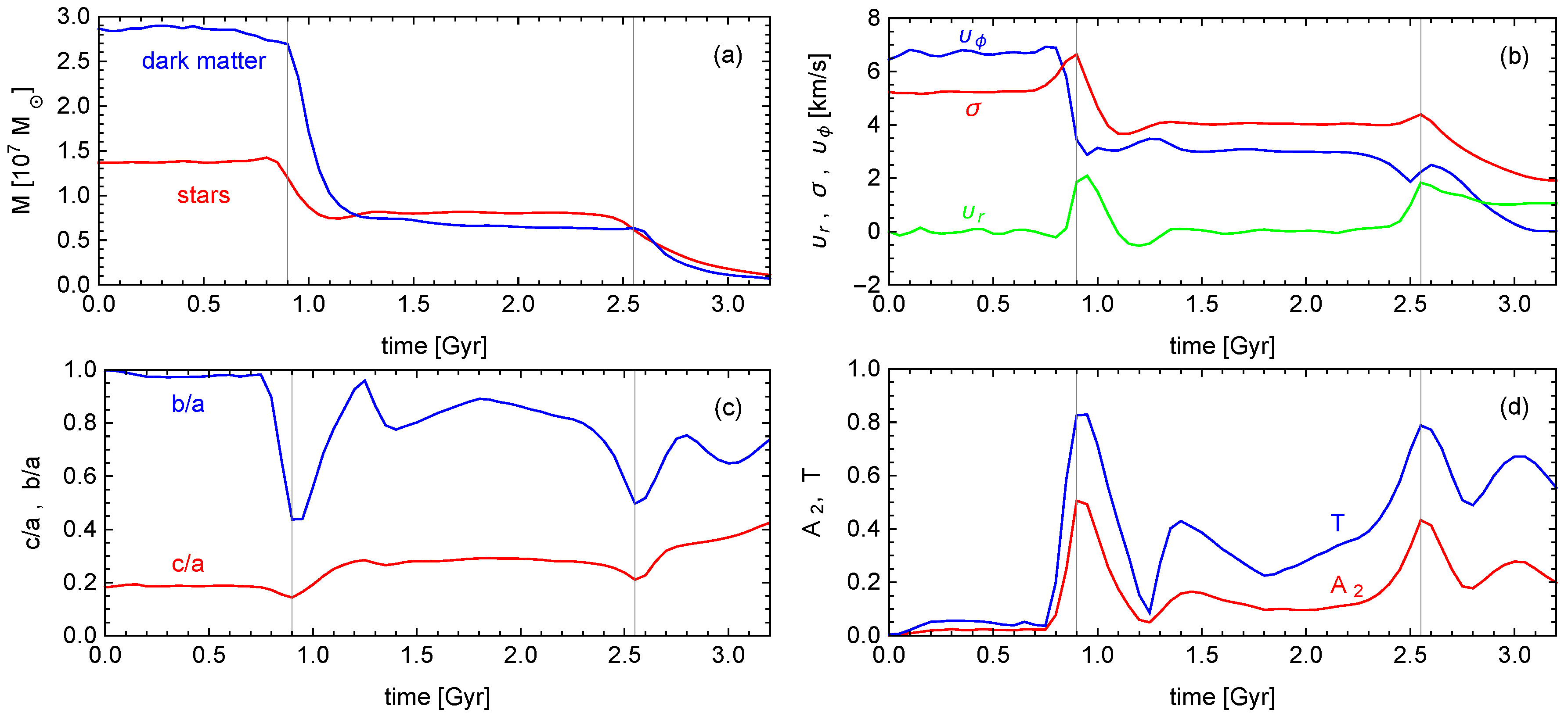
In order to characterize the disruption process in more detail, we have calculated a number of properties of the dwarf for all simulation outputs between
and
Gyr and show them as a function of time in
Figure 4. In all panels, the thin vertical gray lines indicate pericenter passages. The upper left panel plots the mass of dark matter and stars (the blue and the red line, respectively) contained within the 3D radius of 1 kpc from the center of the dwarf. Although the dark matter content dominates over stars by a factor larger than 2 in this region initially, at the first pericenter passage this component is more heavily stripped and afterwards the two are almost equal. However, between the first and second pericenter, the two masses remain constant which means that the dwarf, although heavily stripped, is able to retain its identity and remain a bound system. After the second pericenter, instead, the masses within 1 kpc gradually drop to very small fractions of the initial values: 2% for dark matter and 7% for stars at
Gyr. This means that, at this time, the properties of the dwarf cannot be reliably measured any more and justifies our choice of this time as the time of disruption.
The upper right panel of
Figure 4 describes the evolution of the dwarf’s kinematics. The blue and red lines show the changes of the mean rotational velocity
and the 1D velocity dispersion
σ in time, respectively. The measurements again are done for stars within the radius of 1 kpc using spherical coordinates
r,
θ and
centered on the dwarf, with
defined in the dwarf’s disk plane. While at the beginning
as expected for a rotation-dominated disk, after the first pericenter, the relation is inverted and random motions start to dominate as a result of tidal shocking. After the second pericenter passage, both quantities decrease to low values. The disrupting dwarf stops rotating completely and has a low velocity dispersion. An interesting signature of disruption is the behaviour of the mean radial velocity
within the dwarf. For a system in equilibrium, this quantity should be close to zero, which is indeed the case at the beginning of the evolution. At the first pericenter, the dwarf is stretched with
going up to 2 km·s
but then drops to zero again as the dwarf recovers its equilibrium state. After the second pericenter, however, the value does not drop to zero but remains at the level of 1 km·s
, so the dwarf is slowly expanding. This phenomenon is similar to the one of “exploding satellites” recently discussed in the context of modelling the Hercules dwarf [
23]. In our case, the process seems less violent as a result of a less eccentric orbit.
The two lower panels of
Figure 4 illustrate the evolution of the dwarf’s shape in terms of the axis ratios
and
(with
and
c referring to the longest, intermediate and the shortest axis) of the stellar component (left) and the triaxiality parameter
and the bar mode
(right). The measurements were done again for stars within 1 kpc from the inertia tensor (axis ratios) or by projecting the positions onto the disk plane (
). Initially,
and
as expected for a disk. After the pericenter passage, the dwarf becomes triaxial but close to oblate. At the end of the evolution, it is more prolate as expected for a stream-like disrupting system.
4. Discussion
We performed a simulation of the evolution of a late-type dwarf galaxy in the tidal field of the Milky Way. The dwarf had initially a core-like dark matter distribution and was placed on a typical orbit. We have demonstrated that such a configuration indeed leads to the destruction of the dwarf: it survives the first pericenter passage but gets dissolved after the second. Our results provide an illustrative and convincing example of the process of dissolution of dwarf galaxies with shallow dark matter profiles and confirm other similar findings. The general picture emerging from the present and other studies is that the process of destruction can occur on different orbits and typically more extended ones will allow the dwarf to survive more pericenter passages [
10]. The details of the process depend on the particular dark matter profile of the dwarf. In the case of the dwarf studied here, with a relatively shallow cusp (
) the dwarf is dissolved rather quickly, before it is heavily stripped. It transforms into a long stream with a very shallow density profile. On the other hand, for more cuspy profiles (
), we expect the dwarf to be heavily stripped before it is completely destroyed. Such stripping may be responsible for the formation of ultra-faint dwarfs [
9].
The details of the disruption process we have sketched here deserve further study. Using all the 6D position and velocity data available from the simulation, it is quite straightforward to identify the moment of disruption. It may not be so easy in the case of observed dwarfs when only projected positions and line-of-sight velocities are available. However, being able to distinguish disrupting objects from those that are still gravitationally bound seems to be essential if we want to reliably determine the mass content of dwarfs. All available methods to do so rely on the assumption that the objects are at least in approximate equilibrium [
24]. It has been shown [
25,
26] that accurate mass estimates can be obtained even for heavily stripped and tidally affected dwarfs provided they are still bound and the interlopers in the form of the tidally stripped stars are properly accounted for [
27]. The methods will not work, however, for dwarfs undergoing disruption.
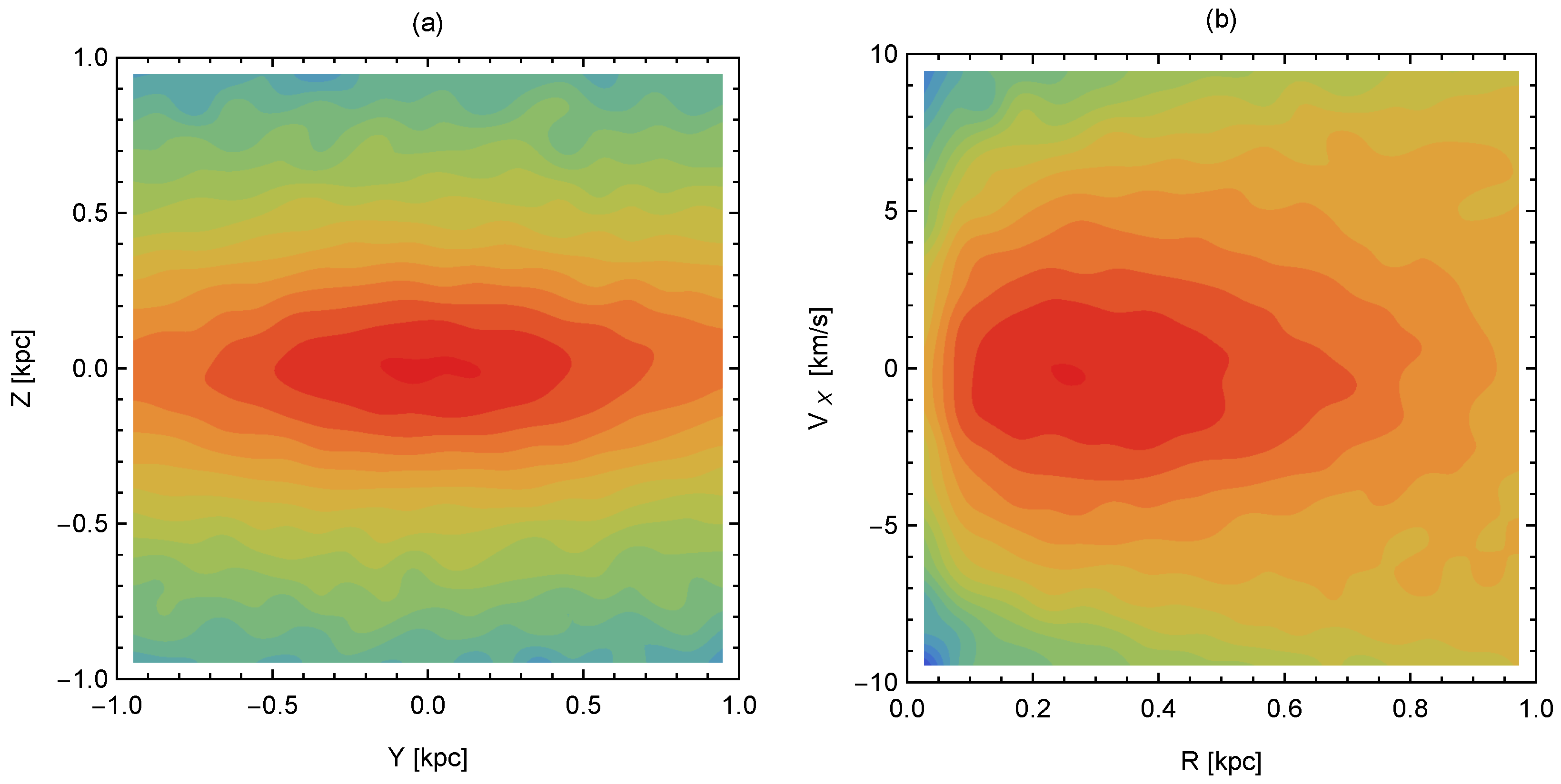
We illustrate the issue using
Figure 5 which shows the observed properties of our simulated dwarf at the time of disruption (
Gyr). For this Figure, we have selected the line of sight of the imaginary observer to be the
X axis of the simulation box, i.e., we may imagine the observer as placed near the host galaxy and looking at the dwarf along the
X axis of
Figure 1. The left panel of
Figure 5 shows the surface density distribution of the stars in the dwarf as it would be seen by such an observer. The image is heavily contaminated by the stars from the tidal tails since those are oriented close to the line of sight. The 2D density profile of such a sample of stars would be steeper than the one projected onto the orbital plane which is very flat (
Figure 3b) and therefore it would be difficult to immediately judge the dwarf as disrupting. In addition, the shape of the distribution, although quite elongated, would be difficult to distinguish from a tidally induced bar which can form in dwarfs orbiting the Milky Way in some configurations [
15,
16]. Such a bar may be responsible for the elongated shape of the Sagittarius dwarf [
28].
The kinematics of the disrupting dwarf is also difficult to distinguish from other cases. The right panel of
Figure 5 shows a phase-space diagram of our simulated dwarf at the same time in the form of the distribution of the velocities along the line of sight (
) as a function of the projected radius
R on the surface of the sky. The density of the stars in the diagram was color-coded so that the red corresponds to the highest density. While the highest-density contours outline the main body of the dwarf quite clearly, the lower-density ones extend further and further from the
line due to the contribution from the tidal tails. However, the diagram would look very similar in the case of a dwarf which still has a bound component but its kinematics is heavily contaminated by the tails or there is a tumbling bar which contributes to the velocity distribution due to its rotation. The described difficulties call for further studies of this issue in order to find features that could discriminate between disrupting and bound dwarfs.


