Abstract
Recent centimeter-to-millimeter monitoring of nearby gamma-ray bursts (GRBs) has revealed late-time (– days) radio rebrightenings and spectral turnovers not explained by standard forward-shock scenarios with steady microphysics. We attribute these features to a buried millisecond magnetar whose surface dipole, initially submerged by early fallback (hours after birth), re-emerges via Hall–Ohmic diffusion on year–to–decade timescales, partially re-energizing the external shock. We combine a minimally parametric analytic framework with axisymmetric magnetohydrodynamic simulations of the hypercritical fallback phase to characterize burial depths and the initial conditions for reemergence. The growth of the external dipole is modeled as and calibrated against physically plausible diffusion timescales –. Spin-down power couples to the afterglow through the surrounding ejecta via a single effective coupling factor and a causal delay kernel, encapsulating mediation by supernova ejecta/pulsar-wind nebulae in collapsars and by merger ejecta/winds in compact-object mergers. Applied to a representative set of events with late-time radio detections and upper limits, our scheme reproduces the observed rebrightenings and turnovers with modest coupling efficiencies. Within this picture, late-time centimeter–millimeter afterglows provide a practical diagnostic of magnetic-burial depth and crustal conductivity in newborn magnetars powering GRB afterglows, and motivate systematic radio follow-up hundreds to thousands of days after the trigger.
1. Introduction
Gamma-ray bursts (GRBs) offer a rare glimpse into the birth of compact objects and the physics of relativistic shocks (e.g., see [1,2]). Beyond their prompt -ray flash, late-time centimeter-to-millimeter emission provides a calorimetric probe of how and when central engines inject energy into the blast wave. Understanding the physical origin of late-time radio rebrightenings is therefore essential both for GRB energy closure and for using GRBs as laboratories of newborn neutron star (NS) magnetism and transport [3]. GRBs are commonly classified into two types: short GRBs ( s), produced by binary NS mergers or NS–black hole (BH) mergers [4,5,6,7], and long GRBs ( s), associated with the collapse of massive stars [8,9,10,11]. Two leading central engine candidates are considered: (i) an accretion Kerr BH, where a transient torus powers the jet via neutrino annihilation or the Blandford-Znajek process [8,9,11,12,13,14]; and (ii) an ultra-fast spinning, highly magnetized NS (a millisecond magnetar), whose magnetic-dipole spin-down provides the required power [4,5,6,7]. In either channel, the collapse or merger ejects fallback material; part of this debris circularizes into a disk and may subsequently reaccrete [15,16,17]. In the magnetar scenario, this inflow can supply additional angular momentum and prolong the spin-down phase [18]. However, excessive accretion may drive the star above the maximum mass, leading to BH formation [19]. Once relativistic jets are launched, internal dissipation produces the prompt emission; the jets then decelerate in the circumburst medium, generating a broadband afterglow via synchrotron radiation of shock-accelerated electrons [1,20,21,22]. Late-time centimeter-to-millimeter observations provide a calorimetric handle on the blast-wave energy and thus a sensitive probe of central-engine activity well after the prompt phase. A subset of nearby events exhibits late-time ( days) radio rebrightenings and spectral turnovers that are difficult to reconcile with a standard forward-shock model with steady microphysics [23,24]. Alternative explanations include refreshed shocks from ejecta stratification, density fluctuations in the circumburst medium, evolving microphysical parameters [25], resurgence of the reverse shock [26,27], and off-axis or structured jet components (e.g., [28,29,30,31,32,33,34,35,36]). Assessing these scenarios is essential to separate external-medium or microphysics effects from genuine late-time energy injection by the central engine.
Soon after birth, a millisecond magnetar is expected to host a surface dipole field G generated by convective dynamos and differential rotation [4,37]. If the remnant undergoes hypercritical fallback at rates , the ram pressure advects magnetic flux into the nascent crust, forming a dense blanket of mass at depths m [38,39]. This “buried-field” configuration suppresses the external dipole moment and the early spin-down luminosity [40,41,42]. The submerged field subsequently diffuses outward through coupled Hall drift and Ohmic dissipation in the hot, impurity-rich crust. In this work, we combine a minimally parametric analytic description of the reemergence with axisymmetric hydrodynamic and magnetohydrodynamic (MHD) simulations of the hypercritical fallback phase, which constrain plausible burial depths and geometries and define the initial conditions for the growth of the external dipole. For shallow burial ( m) and high conductivities (), the emergence timescale can reach [43,44,45,46]. Throughout this work, we encapsulate the macroscopic growth of the external dipole in a dimensionless function , which represents the reemergence driven by Hall-Ohmic diffusion (Section 2).
In GRBs that leave a long-lived magnetar, the time-dependent spin-down power couples to the external shock through the surrounding ejecta. In collapsars, the energy is first injected into a pulsar-wind nebula (PWN) embedded within expanding supernova (SN) ejecta before leakage into the circumburst medium. In compact-object mergers, the coupling proceeds through dynamical ejecta and magnetar-driven winds. We model this mediation with a single effective coupling factor and a causal delay kernel that encapsulates diffusion through the bulk ejecta and leakage of magnetar wind energy via low–optical–depth channels (jet-carved funnels/cocoon interfaces) ([7,47,48,49] and references therein). Our formulation remains agnostic to detailed radiative-transfer and jet-structure modeling; instead, the coupling factor and delay kernel provide a phenomenological bridge from the central engine to late-time radio observables.
A time-dependent increase of the spin-down luminosity due to magnetic reemergence modifies the afterglow once the blast wave becomes mildly relativistic, shifting characteristic synchrotron frequencies and potentially producing radio rebrightenings and spectral turnovers on – d timescales. Here we test whether fallback-driven submergence and Hall–Ohmic reemergence of the external dipole in a millisecond magnetar can account for these late-time radio features. Anticipating our main conclusion, we find that delayed energy release with – and modest coupling to the forward shock reproduces the observed rebrightenings and turnovers in nearby events, implying that centimeter–millimeter afterglows can diagnose crustal transport and magnetic-burial depth in newborn NS.
On the other hand, time-of-flight searches for Lorentz-invariance violation (LIV) predict an energy-dependent photon speed, leading to arrival-time lags that scale with energy and distance. GRBs provide stringent constraints on such vacuum dispersion: already the seminal proposal of Amelino-Camelia et al. [50] motivated GRB tests, and Fermi–LAT observations (e.g., GRB 090510) set limits as strong as for linear LIV and for quadratic terms [51]. TeV detections by MAGIC (GRB 190114C) and the exceptional GRB 221009A further tightened the bounds, with no evidence for propagation-induced delays [52,53]. In this study, the delays we model are source-side, macroscopic, and effectively achromatic. These delays arise from the coupling of magnetar spin-down to the afterglow through the surrounding ejecta, which we refer to as our causal delay kernel. Given the current LIV limits, any vacuum-dispersion lag at radio/X-ray energies is negligible compared to the year-scale source delays considered here; accordingly, we do not include LIV terms in our light-curve modeling.
The paper is organized as follows. Section 2 develops our analytic and numerical framework for the magnetic-field submergence and reemergence, including the definition of and its calibration. Section 3 presents the synchrotron dynamics of the external shock under delayed energy injection, discussing the pre- and post-reemergence regimes, including the deep Newtonian phase. In Section 4, we present a brief discussion. In Section 5, we apply the model to a representative set of nearby GRBs with late-time radio coverage. Section 6 summarizes the main results and prospects.
2. Analytical and Numerical Framework for Magnetic-Field Submergence and Reemergence
2.1. Magnetic-Field Submergence Beneath the Magnetar Crust
Hypercritical fallback accretion at rates is expected during the first after core collapse or compact-binary merger. It deposits a quasi-hydrostatic envelope of mass on the nascent NS, as indicated by numerical simulations (e.g., see [7,10,11,46]). Two- and three-dimensional simulations show that the ram pressure of this envelope overwhelms the magnetic tension of a dipole, advecting the field to depths where densities reach [46,54,55]. Both free-fall and quasi-hydrostatic initial conditions yield the same qualitative outcome in our axisymmetric runs: rapid confinement of external flux beneath the newly accreted crust within , with only weak sensitivity to the initial loop geometry explored.
Early analytical studies had already outlined this hidden-field channel [38,41], and magneto-thermal models predicted only a weak dependence of the burial fraction on the seed field strength [56]. These results indicate that submergence is a generic consequence of fallback whenever the gravitational binding energy of the inflow exceeds the magnetic energy stored above the stellar surface. The same conclusions apply to millisecond magnetars, widely considered central engines for a subset of observed GRBs.
Figure 1 summarizes the hypercritical fallback phase that precedes magnetic burial in a newborn millisecond magnetar. The left-hand panel schematically shows accretion onto the proto-magnetar at a rate . The flow is decelerated at the accretion–shock radius – and builds a quasi–spherical envelope above the neutrinosphere, i.e., the neutrino decoupling surface where the optical depth falls to and neutrinos free–stream (–). Within the gain region, charged-current interactions deposit energy that partly offsets the ram pressure, while large-scale overturn redistributes entropy and advects magnetic flux to depths of . The right-hand panel displays a 2D hydrodynamic snapshot from a FLASH simulation at [57]. Four diagnostic wedges display, clockwise from the top, the mass density, thermal pressure, total specific energy, and electron-flavor neutrino emissivity. The high-density/pressure ring centered at marks the onset of quasi-hydrostatic balance and significant neutrino cooling. Below this ring, a low-energy, high-emissivity zone suggests the formation of a dense proto-crust on the magnetar surface. These features support the analytical picture: the shocked fallback flow creates a neutrino-cooled shell that both obscures the external dipole and establishes the thermal boundary conditions for Hall-driven reemergence on timescales of decades.
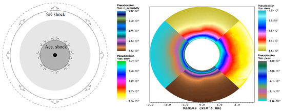
Figure 1.
Schematic and simulation of hypercritical fallback onto a newborn millisecond magnetar. Left: cartoon of the accretion geometry. Material falling back at is decelerated at the accretion shock radius ; below the shock an atmosphere in near hydrostatic equilibrium—cooled by neutrino emission—deposits mass and thermal energy onto the star during the first few hours after core collapse, while convective overturn advects magnetic flux downward and initiates field burial. Right: 2-D hydrodynamic snapshot computed with the flash code ( ms). The circular wedge is divided into four diagnostic panels: top—mass density; left—thermal pressure; bottom—electron-type neutrino emissivity; and right—total specific energy. Together they illustrate the formation of the quasi-hydrostatic envelope and the build-up of a dense proto-crust at the magnetar surface.
Figure 2 displays four snapshots from our two-dimensional, neutrino-assisted MHD simulation performed with FLASH. The columns correspond to , 1, 10, and after the onset of fallback and cover the region above the magnetar surface. Top row—density: A dense accretion blanket forms almost instantaneously. By , Rayleigh–Taylor fingers appear, and by they pervade the envelope, indicating vigorous mixing. Middle row—: We plot the ratio of magnetic pressure, , to ram pressure, . Except within the initial magnetic arch (visible at ), the ratio remains throughout the envelope, demonstrating that infalling matter dominates the force balance and drives complete magnetic submergence. The transient patches with are shredded and advected downward, disappearing with . Bottom row—temperature: Cooler, neutrino-dominated material settles at the base, while hotter gas is mixed upward by overturn motions, establishing the expected negative temperature gradient. Multicolor iso-contours of magnetic-field strength are overplotted in every panel, tracing the steady downward advection and distortion of the dipolar flux. By , the external field is confined within a layer beneath the interface, consistent with analytic predictions and one-dimensional calculations [38,56]. These snapshots illustrate how ram-pressure-dominated burial reduces the surface field and establishes the initial conditions for its subsequent evolution. The final burial depth is primarily determined by the total accreted mass and the local equilibrium between magnetic stress and hydrostatic pressure. One-dimensional estimates give [56], in agreement with multi-D MHD simulations of hypercritical fallback that find variations in when the pre-existing dipole is varied from to G [46,54,56]. Because is set by the fallback light curve rather than by the proto-magnetar field, the early spin-down luminosity is quenched almost irrespective of the prompt dynamo strength. Notably, the crust that seals the field is both hot ( K) and impurity-rich, conditions that foster rapid Hall drift and enhanced Ohmic diffusion; these processes will later mediate field reemergence on timescales of a few to a few tens of years, thus linking the accretion history to delayed energy injection in GRB afterglows.
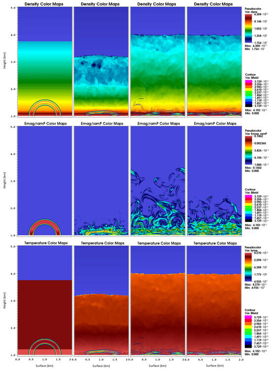
Figure 2.
Time evolution of magnetic-field burial in a newborn millisecond magnetar subject to hypercritical fallback. Columns correspond to , 1, 10 and 100 ms. Top: density colour maps revealing the growth of a Rayleigh–Taylor–unstable envelope and the initial build up of a dense proto crust on the stellar surface. Middle: maps of the pressure ratio ; values confirm that ram pressure dominates the dynamics and forces the dipolar field to submerge. Bottom: temperature maps highlighting the neutrino–cooled layer that forms near the stellar surface as the envelope settles. In every panel, multicolour iso–contours of magnetic-field strength are over-plotted, tracing the progressive downward advection of dipolar flux to depths of m.
Magnetic-field geometry and robustness: For simplicity, our simulations adopt an initially surface-anchored magnetic loop as a proxy for a dipole. This choice does not determine the outcome of the burial. Multidimensional calculations show that, under strongly hypercritical fallback, the external field is rapidly advected and submerged beneath the forming crust regardless of the seed topology–including uniform horizontal/vertical fields, vertical gradients, and loop-like structures–and irrespective of whether the envelope starts in free fall or in quasi-hydrostatic equilibrium [46,54]. The resulting confined geometry is similar across these sets of conditions, with magnetic flux transported to depths of order – cm on subsecond timescales. In this work, we therefore use a loop configuration for computational economy and interpret the reemergence, via the growth law , as the effective revival of the large-scale (low-order) external dipole that governs the spin-down power and couples to the afterglow emission. Higher-order or toroidal components primarily renormalize the phenomenological parameters without altering the late-time radio signature modeled here.
2.2. Crustal Magnetic-Field Evolution in Millisecond Magnetars
Millisecond magnetars differ from ordinary NS by their ultra-short spin periods and strong surface dipoles, G [4,37]. Most studies focus on the large-scale dipole, yet the configuration of the crustal field is equally important for thermal, mechanical, and radiative evolution [38,41,58,59]. Rapid rotation, intense magnetic pressure , and early hypercritical fallback create hot, impurity-rich crusts [7,42,54,56,60,61]. Such conditions accelerate Hall drift (non-dissipative advection of the magnetic field by the electron fluid with timescale ) and Ohmic diffusion (resistive decay with ), as well as plastic yielding, thereby setting the timescale over which a buried dipole can re-emerge [62,63,64].
2.2.1. Induction Equation
Magnetic evolution in the solid crust obeys the Hall–Ohmic equation [59,64,65,66]
where the first (Hall) term is non-dissipative but transfers energy to small scales that the second (Ohmic) term dissipates [56,67]. For G the Hall timescale rivals or beats the Ohmic time [68].
2.2.2. Characteristic Timescales
Using the conductivity tables of Chamel and Haensel [69] at K (a hot, impurity-rich crust just after fallback), a representative electrical conductivity is . The corresponding Ohmic time is
with L the burial depth. This normalization reflects the high-T/high- regime relevant immediately after hypercritical accretion; as the crust cools and purifies, increases toward – [69], lengthening the purely Ohmic time [38,70].
Hall drift operates more rapidly and transports flux to smaller length scales,
where is the electron number density. For the same physical L used in Equation (2), the scaling in (3) can be applied directly (e.g., km yields yr for the fiducial and B). Because , magnetar-strength fields naturally produce sub-annual Hall evolution at –1 km.
The global reemergence time is generally shorter than because Hall drift transfers magnetic energy to smaller structures of size , for which the local Ohmic time scales as . For the fiducial numbers in Equation (2), reduces the Ohmic time by (to yr), and brings it to yr, consistent with a decade-scale once Hall-driven cascades and localized yielding are active. This motivates the parametric treatment adopted in Section 2.3, where reflects the net outcome of Hall transport, local heating, and Ohmic dissipation at the effective scale ℓ set by the crustal dynamics.
2.2.3. Thermal Relaxation and Thermo-Magnetic Feedback
During the first – yr a newborn magnetar cools from K to ≲ K as its crust and core approach thermal equilibrium [56,71]. Because both the electrical conductivity and the Hall parameter scale as , the advancing cooling front progressively freezes the magnetic configuration. Hall drift is efficient while the crust remains hot but weakens once K, whereas the Ohmic time (2) lengthens.
When magnetic energy is lost faster than neutrinos can carry it away, Joule heating rewarms the lattice and partially offsets the drop in conductivity [72,73]. This thermo-magnetic feedback can delay crustal relaxation by several decades and preserve a larger reservoir of electromagnetic energy, thereby amplifying any late-time energy injection into the afterglow.
2.2.4. Local Breakthroughs and Feedback
Three-dimensional simulations reveal that Hall cascades, coupled to plastic flow (irreversible viscoplastic creep once magnetic/Maxwell stresses exceed the crustal yield) or thermoplastic flow (thermally activated, self-propagating failure fronts—‘thermoplastic waves’), can breach the crust locally on month–to–year timescales [44,74,75]. Lateral heat transport accelerates diffusion in Hall-active regions [72,73], and magnetic stresses can trigger fractures once exceeds the yield strength [76]. The resulting plastic flow can then advect the flux outward [77,78]. Combined Hall–Ohmic transport, heating, and crustal failure permit partial reemergence within a few years—even if the global dipole resurfaces more slowly—and may help explain late X-ray and radio bumps in several GRBs [79,80,81,82,83].
2.2.5. Microphysical Uncertainties: Conductivity, Cooling, and Impurities
The effective Ohmic diffusion timescale on a crustal length L is , with magnetic diffusivity . Conductivity is controlled by electron scattering off phonons and impurities: at high temperature the phonon contribution dominates (resistivity increasing with T), whereas as the crust cools, the phonon term freezes out and temperature-independent electron–impurity scattering, parameterized by the dimensionless impurity parameter (with the number fractions and the charge average), which measures lattice disorder and dominates electron–impurity scattering, implying in that regime [63,64]. Consequently, cooling tends to lengthen , while a larger impurity content (higher ) shortens it. The Hall timescale scales as , so stronger fields and/or lower electron densities accelerate Hall drift (shorter ). Within our modeling framework, these microphysical effects are phenomenologically absorbed into the growth law : should be interpreted as an effective emergence timescale that integrates the combined Hall–Ohm evolution along a plausible thermal history, while captures Hall-driven acceleration. The inferred range yr is thus an observationally calibrated timescale, robust to reasonable NS structure variations, yet still degenerate with the poorly known . Joint 1–100 GHz light curves combined with VLBI size constraints and, when available, polarimetry can help break the degeneracies and translate into constraints on crustal transport coefficients.
In summary, the fastest end of the parameter space corresponds to –10 yr, enabled by rapid Hall transport () and Ohmic dissipation at scales in a hot, impure crust. A decade-to-few-decade reemergence is a plausible outcome for newborn millisecond magnetars as the crust cools and grows, a regime we model with the parametric model of Section 2.3.
2.3. Magnetic-Field Reemergence: A Unified Parametric Model
When hypercritical accretion stops, the external dipole of a newborn magnetar diffuses through the crust and grows from a buried value toward a saturated strength on year–decade timescales, driven by Hall transport and Ohmic dissipation modulated by local thermodynamics and composition (Section 2.2). To capture this evolution without resorting to full 3D simulations, we adopt a compact parametric description that unifies the exponential, hyperbolic, and slow power-law emergences used in earlier work.
2.3.1. Unified Growth Function
We define the dimensionless growth function as
so that the surface dipole becomes and the torque scales as .
A unified form that smoothly interpolates between common prescriptions is
where is the effective emergence time (set by the Hall–Ohm interplay; Section 2.2.2) and controls the shape of the growth (fast/exponential for , progressively slower as ). By construction, and .
Note that Equation (5) provides a unified mapping of the above templates, recovering the three functional forms employed previously,
and thus subsumes the exponential, hyperbolic, and power-law growth laws discussed in Bernal et al. [84] without changing any subsequent afterglow calculation.
2.3.2. Spin-Down with a Time-Dependent Field
For a constant braking index n (with for ideal dipole radiation), the spin evolution reads
where R is the NS radius, I its moment of inertia, and the magnetic obliquity. Integrating Equation (7) for gives
It is convenient to define the instantaneous characteristic timescale
where is the initial characteristic time. For Equation (9) reduces to the standard constant-field case.
The rotational energy loss is
where . During growth (), the effective braking index satisfies
so can drop below n while increases.
2.3.3. Physical Interpretation and Parameter Space
The triplet captures the crustal transport and burial depth in a hot, impurity-rich magnetar crust:
- represents the Hall–Ohm emergence time (Section 2.2.2). Our calibration adopts the regime K introduced by Chamel and Haensel [69] with conductivities – (cgs) appropriate for early, impurity-rich conditions and burial depths informed by the MHD simulations (–1 km). In this regime, decade-scale emergences are natural once Hall transport cascades to small scales ().
- quantifies the relative importance of rapid Hall-driven acceleration versus slower Ohmic relaxation: small yields faster, near-exponential growth; yields slower, power-law–like emergence expected for deeper burial or cooler, purer crusts [56].
- encodes the burial depth set primarily by the fallback mass and the local balance of magnetic and hydrostatic stresses (Section 2.1).
Within this framework, the late-time energetics are largely insensitive to the exact functional form once , but the timing and amplitude of the rebrightening depend on the early growth rate (hence on and ), which we will constrain with the radio data.
2.3.4. Advantages of the Unified Model
Relative to using separate exponential/hyperbolic/power-law prescriptions, Equations (5)–(10) (i) provide a single smooth family with well-defined limits; (ii) ensure correct normalization and ; (iii) keep the torque proportional to by construction (); and (iv) link directly to the timing observables through and . Throughout the remainder of this work we treat as free, data-driven parameters, while and follow from the initial spin and .
Figure 3 quantifies how the magnetic-field growth law controls both field revival and spin-down power. The left-hand panel follows the surface field as it rises from its buried value, (i.e., for ), toward the magnetar strength over the mergence timescales –. The right-hand panel shows the corresponding spin-down luminosity obtained from Equation (10); the rapid rise in marks the transition from a fall-back-dominated to a magnetar-dominated energy budget and sets the epoch when a late-time centimeter-millimeter rebrightening is expected (Section 3). We show three analytical prescriptions: pure exponential growth (), an intermediate case (), and a slow power-law–like rise ()—which map to the exponential, hyperbolic and power-law templates used in earlier work. All three track nearly the same evolution once (field saturation), indicating that late-time energetics are largely insensitive to the exact functional form; however, the early growth rate, fast for and progressively slower as —imprints distinct signatures on both the timing and the amplitude of the subsequent radio afterglow.
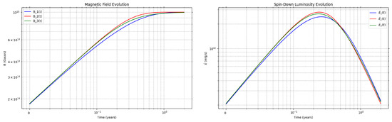
Figure 3.
Early magnetic-field revival and its radiative imprint. Left: Evolution of the surface dipole for the unified growth law of Equation (5), with burial fraction , emergence timescales –10 yr, and saturation at G. Right: Corresponding spin-down luminosity from Equation (10); the rapid rise of marks the transition from fallback-dominated to magnetar-dominated energy injection and sets the epoch at which a late-time centimeter–millimeter rebrightening is expected (see Section 3). Both panels display three analytic prescriptions parameterized by —exponential (), hyperbolic-like (), and slow power-law–like (; shown in blue, red, and green, respectively). While the curves converge to the same plateau once (field saturation), the early growth rate leaves distinct imprints on the timing and amplitude of the subsequent radio afterglow.
Our results depend primarily on the existence of a single effective emergence timescale rather than on the detailed kernel shape: replacing k with other normalized, single–timescale causal forms (exponential or lognormal/gamma) at fixed parameter count yields consistent fits and within the statistical uncertainties. Beyond the no–burial baseline, we also considered density–jump and refreshed–shock scenarios; these do not reproduce both the amplitude and the optically thin spectral slope of the late–time cm–mm bumps without introducing extra parameters, hence we adopt the minimal, kernel–driven reemergence model.
2.3.5. Ejecta–to–Shock Coupling: Minimal Interface
The magnetar spin-down power does not immediately couple with the external forward shock. Energy must first traverse the surrounding ejecta—SN ejecta/pulsar-wind nebula (PWN) in collapsars and dynamical ejecta plus magnetar-driven winds compact object mergers—before any leakage into the circumburst medium [47,48,49]. We encapsulate this mediation with a single effective coupling factor and a causal delay kernel ,
where is given by Equation (10). By construction and has units of , so that carries units of power. This provides a phenomenological bridge from internal-field growth to late-time radio observables without detailed radiative transfer.
For concreteness, we adopt two minimal choices that bracket plausible channels:
with H the Heaviside function. In collapsars, implicitly accounts for PWN→ejecta work and collimation losses; in mergers, it captures absorption in dynamical ejecta and magnetar-driven winds. Parameters and represent, respectively, an effective advection/escape time and a diffusive leakage timescale through the ejecta/coin.
Unless stated otherwise, we adopt a constant and a small effective delay ( or ), so that up to a slight change or smoothing of time. This keeps the late-time energetics controlled by the growth law while acknowledging ejecta mediation in a minimal and reproducible way.
2.3.6. Separable Coupling Ansatz and Its Regime of Validity
We model the power injected into the blast wave as the spin-down luminosity reprocessed through a causal, source-side delay kernel and scaled by a single effective coupling efficiency,
where is causal ( for ) and normalized (), and captures the fraction of the magnetar output that ultimately couples to the forward shock (rather than being stored or thermalized in the ejecta or PWN). In the deep-Newtonian phase and for a quasi-homogeneous external medium, shock microphysics varies slowly, so time-independent is a good first-order approximation; it primarily sets the overall amplitude, whereas the shape and timescale of the rebrightening are governed by the kernel. If the efficiency evolves slowly, with , the resulting injection rate reads as
i.e., a mild, smooth amplitude drift superimposed on the kernel-driven profile. In the order constrained by our data, such drifts are observationally degenerate with global normalization (absorbed into and ), while the emergent timescale remains robust. Consequently, we adopt the separable ansatz (15) throughout and interpret as the effective reemergence timescale of the external dipole of low order (Section 2.1).
3. Theoretical Approach: Dynamics of the GRB Afterglow and Synchrotron Light Curves
The behavior of the decelerated material interacting with the external environment for several years is predicted to remain inside the nonrelativistic domain, thereby aligning with the Sedov–Taylor solution. Recently, Fraija et al. [85] showed the synchrotron light curves produced by the deceleration of sub-relativistic material before and after the reemergence of the magnetic field. The authors considered a quasi-spherical material ( with the fiducial energy [86] and the PL index of the velocity distribution) interacting with a constant density medium. Here, we extend the dynamics of the afterglow nonrelativistic model with constant density () considering the Deep Newtonian regime.
3.1. Synchrotron Light Curves Before B-Reemergence
During the first stage of expansion, the ejecta mass is unaltered by the circumburst environment [87], leading to a uniform velocity () and an increasing radius (). During this stage, the timescales of the magnetic field and the spectral breaks of the electron Lorentz factors are , and , respectively. Prime and unprimed quantities will be used to represent the comoving and observer frames, respectively. Similarly, the timescales of the spectral breaks and the maximum flux of synchrotron mechanism are , , and , respectively. For , the synchrotron light curve is characterized by fast cooling, but in the opposite case, it exhibits gradual or slow cooling. Therefore, the timescales of the long-lasting light curves of the synchrotron mechanism are for , for and for during fast-cooling regime. During the slow-cooling regime, and for , for and for during the slow-cooling regime.
During the deceleration phase, the velocity and radius of the blast wave evolve as and , respectively. Likewise, the magnetic field in the post-shock zone is proportional to . It should be noted that throughout the shock event, a certain amount of the total energy is persistently transmitted to amplify the magnetic field strength through the microphysical parameter . During the deceleration phase, the breaks of the electron Lorentz factors evolve as and , the characteristic, the cooling and the self-absorbed spectral frequencies vary as , , , and , respectively. Finally, the spectral peak flux density evolves as .
During the Deep Newtonian phase (), the timescale of the magnetic field at the post-shock region becomes . The Lorentz factor of the electrons with the highest energy, which are effectively cooled by synchrotron emission, are
with z the redshift, and the equipartition parameters, and Y the Compton parameter (e.g., see [34]). The associated synchrotron breaks are provided as
The synchrotron breaks in the self-absorption domain are
The maximum flux of synchrotron radiation becomes
with the luminosity distance. Requiring the break frequencies (Equations (18) and (19)) and the maximum flux (Equation (20)), the synchrotron light curves and the closure relations () with the reemergence of magnetic field evolving in the deep Newtonian phase are listed in Table 1. The PL index p corresponds to the spectral index of the electron distribution. We consider the cooling conditions , and and the deceleration of the material in constant density. It is worth noting that the cooling conditions correspond to the order of each spectral break in the synchrotron light curves. From left to right, this table shows the cooling condition, the PL indices of spectral (), the temporal (), and closure relation (). When the PL index of the velocity distribution gets close to , the evolution of the synchrotron light curves reproduces the light curves of the uniform afterglow of a non-spherical material.

Table 1.
Temporal PL indexes of synchrotron light curves and spectra together with the closure relations () of the afterglow density-constant model during the Deep Newtonian phase. The synchrotron light curves do not consider the reemergence of magnetic field.
3.2. Light Curves After B-Reemergence
Analytical synchrotron light curves with and can be obtained for the exponential function type one (, Equation (6)). In this scenario, the luminosity of spin-down is . During the deceleration phase (), the post-shock magnetic field evolves as , and the minimum and cooling Lorentz factors of the electron population are , respectively. The timescales of the synchrotron spectral breaks are , , , and . Finally, the spectral peak flux density evolves as .
In the Deep Newtonian phase (), the timescale of the post-shock magnetic field varies as . The Lorentz factors of the electrons with the lowest energy and the electrons with the highest energy, which are effectively cooled by synchrotron emission, are
The synchrotron spectral breaks are
The synchrotron breaks in the self-absorption domain are
The spectral peak flux density is
Requiring the break frequencies (Equations (22) and (23)) and the maximum flux (Equation (24)), the synchrotron light curves and the closure relations () with the reemergence of magnetic field evolving in the Deep Newtonian phase are listed in Table 2. We consider the cooling conditions , and and the deceleration of the material in constant density. From left to right, this table shows the cooling condition, the PL indices of spectral (), the temporal (), and closure relation (). When the PL index of the velocity distribution gets close to , the changes in synchrotron flux match the behavior of the uniform afterglow of a non-spherical material.
Table 2.
Temporal PL indexes of synchrotron light curves and spectra together with the closure relations () of the afterglow density-constant model during the Deep Newtonian phase. The synchrotron light curves consider the reemergence of magnetic field.
3.3. Analysis of the Light Curves
In Figure 4, we illustrate the parameter-dependent variations in afterglow emission across six panels, where each panel corresponds to the change in a given parameter while keeping the others fixed. The energy bands are color-coded: X-ray (gray), optical (brown), and radio (yellow). In the upper left panel, we present a variation in the kinetic energy ( erg versus erg), which shows that a larger boosts the flux across all bands, with optical/radio exhibiting the largest early-time differences (of around two orders of magnitude). The peak at days is less prominent at larger , and fluxes converge at late times as shock deceleration redistributes energy. In the middle-left panel, we contrast two values of the circumburst density ( cm−3 versus cm−3). A higher density enhances the flux (most notably in X-rays, producing brighter, earlier peaks). It has a modest effect on optical emission, while radio emission shows minimal sensitivity to changes in density. In the lower-left-hand panel, we vary the electron energy fraction ( versus ). At early times, the X-ray flux corresponding to the smaller dominates, but its early peak at day is eventually surpassed as the light curve from the larger continues rising and plateauing at greater values.
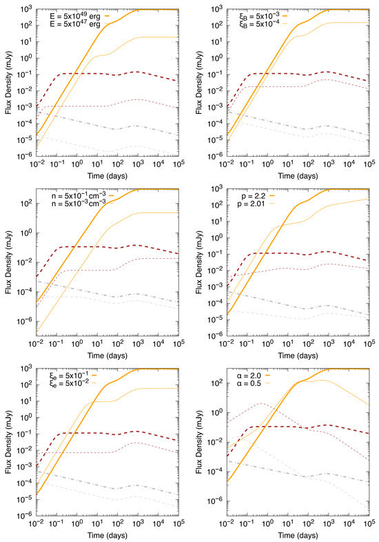
Figure 4.
Synchrotron light curves at X-ray (gray), optical (brown) and radio (yellow) bands generated by the deceleration of the non-relativistic material in the external environment. The light curves of X-ray, optical and radio bands are estimated at 1 keV, 1 eV and 10 GHz, respectively. The parameters used for the emergence of B-field model are: , , , . Each panel shows the variation of one parameter sequentially in our afterglow scenario, but keeping others fixed. In general these values are: E , , , , , .
The optical and radio bands are similarly affected, maintaining a constant difference in the flux between the different cases throughout their evolution. The higher electron energy fraction () consistently dominates in these lower-energy bands. Similar trends are observed in the upper right panel for magnetic field variations: the higher energy fraction, , enhances synchrotron radiation, resulting in a brighter afterglow. In the middle right panel, we examine the variations in the electron spectral index (p). The early light curves show minimal differences because the cooling regimes are initially independent of p. At later times of the evolution, a smaller spectral index generally leads to a more considerable flux. In this case, the lower energies are more sensitive to this difference, and variations can be observed early on at , while in the X-ray band only until . Finally, the lower right panel shows that smaller values of sharpen both the rise and the decline of the light curves, increasing the early-time flux while suppressing late-time emission across all bands.
Figure 5 differs from Figure 4 in the choice of the velocity structure index , using (corresponding to jet-like dynamics) instead of (which models a quasi-spherical outflow). This parameter variation fundamentally alters the shape of the light curves across all bands. The case produces substantially brighter early-time emission, which exceeds the case by over two orders of magnitude, with earlier flux peaks in all bands. This behavior reflects rapid energy injection, particularly noticeable in the X-ray band. On the other hand, the model in Figure 4 shows that a slower rise in flux leads to a more sustained injection of energy over time, resulting in a flatter decay at late times. Consequently, the light curves in Figure 4 maintain a higher late-time flux than those in Figure 5, where steep declines occur after the initial rapid energy injection.
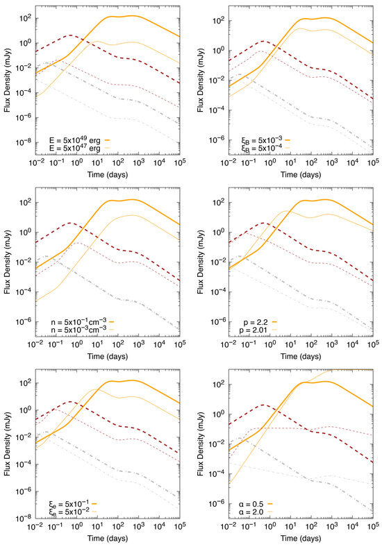
Figure 5.
The same as Figure 4, but for .
In Figure 6 and Figure 7, we observe how variations in magnetic-field evolution parameters impact the afterglow emission. The parameters we vary include the diffusion timescale , the initial spin-down time , the growth efficiency , the initial spin-down luminosity and the times marking the start and end of the emergence process and , respectively. The top-left panel shows variations in (1.5–3.0 yr), where shorter leads to a faster and more pronounced rise in the late-time light curves (most visibly in X-rays), indicating a rapid field reemergence. The middle-left panel reveals that longer delays the peak flux (particularly in the optical/radio bands) by extending the magnetar energy injection. In the bottom-left and upper-right panels, we observe that or significantly increases the flux, particularly in the X-ray/optical bands. Meanwhile, changes in and (middle-right and bottom-right panels) primarily shift the timing of the peak, with earlier starts producing the most noticeable changes across all bands. When we compare Figure 6 and Figure 7, we see that the conclusions for Figure 4 and Figure 5 remain unchanged.
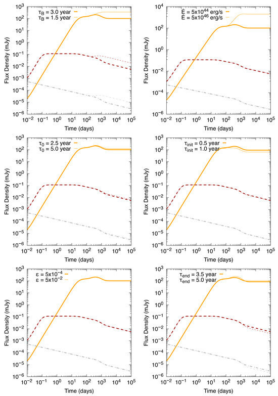
Figure 6.
Synchrotron light curves at X-ray (gray), optical (brown) and radio (yellow) bands generated by the deceleration of the non-relativistic material in the external environment. The light curves of X-ray, optical and radio bands are estimated at 1 keV, 1 eV and 10 GHz, respectively. The parameters used for the afterglow scenario are: , , , , , . Each panel progressively displays the changes of just one parameter in the emergence of B-field model. In general, these values are: , , , .
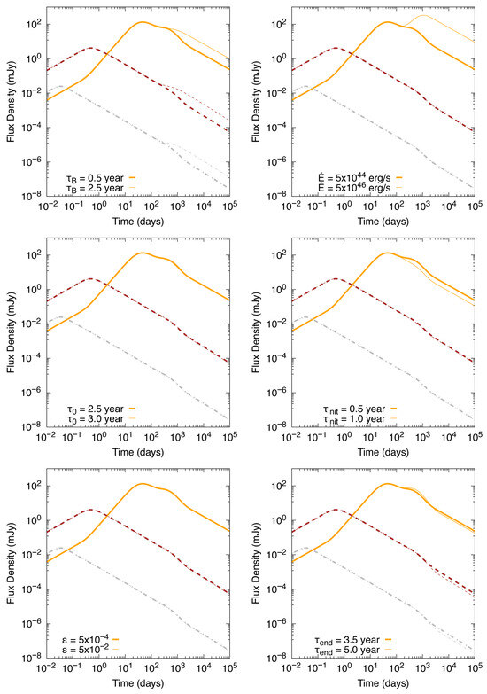
Figure 7.
Same as Figure 6, but for .
Figure 4, Figure 5, Figure 6 and Figure 7 illustrate that various combinations of parameters could yield similar light curves. It should be noted that the equations derived for the afterglow scenario exhibit degeneracy in certain parameters, allowing similar results to be achieved with a different set of values. It can be observed that a more energetic explosion occurring in a rarer medium can generate a radio flux comparable to that of a less energetic explosion in an environment with a higher density. Consequently, alternative physical models, including a refreshed shock model, cannot be conclusively excluded from consideration. As a result, it remains challenging to assert with certainty that the newly introduced physical component is the only viable explanation.
4. Discussion
While substantial, the hypercritical accretion onto the proto-magnetar does not reach the accretion rates necessary to induce gravitational collapse into a BH. Specifically, although accretion provides an additional energy source, the material deposition and resulting increase in rotational energy do not sufficiently destabilize the magnetar. Studies show that for a magnetar to collapse, the critical mass threshold would need to be exceeded under conditions that significantly increase the proto-magnetar’s rotational frequency or density to a level unsustainable by its internal structure [7,88,89]. In hypercritical accretion regimes, where rates of are common, the accreted mass typically does not exceed over the relevant timescales, maintaining the stability of the system [16,17]. Thus, the rotationally supported magnetar remains below the critical point for collapse, even when accounting for the energy contributions of fallback accretion [18,46]. Furthermore, simulations of magnetar evolution under hypercritical accretion [38,56] indicate that the transient crustal submergence of the magnetic field does not alter the overall mass distribution significantly enough to disrupt the NS’s equilibrium, which is crucial in delaying any potential collapse. Therefore, this model suggests that hypercritical accretion onto a proto-magnetar can fuel late-time activity without inevitably leading to a BH transition.
Since hypercritical fallback accretion onto a proto-magnetar does not inherently lead to gravitational collapse, scaling fallback parameters from newborn NSs to millisecond magnetars offers a framework for understanding delayed magnetic reactivation in these objects. The scaling process involves adjusting critical parameters, such as the accretion rate, crustal composition, and thermal diffusion timescales, to reflect the unique energy and density profiles of proto-magnetars. For instance, in magnetars, the fallback accretion rate, typically on the order of over the initial seconds to minutes post-burst, can be translated to yield comparable energy output but with extended diffusion timescales due to the greater rotational energy and magnetic field strength [38,56]. This modified approach implies that the crustal dynamics and field diffusion will scale with both the magnetar’s initial spin rate and its intense magnetic field, allowing the reemergence timescale to be delayed by several years, consistent with the observed X-ray rebrightening in sources like GRB 170817A [82,83]. Importantly, our model assumes that thermomagnetic processes and crustal fractures facilitate this magnetic diffusion. These processes have been observed in simulations of NSs and can be extrapolated to the proto-magnetar case by assuming parameter values that reflect enhanced magnetic and rotational energy. Despite the robust fallback accretion phase, the extraordinary magnetic field strength of the magnetar introduces substantial magnetic pressures and stresses within the newly formed stellar crust. This crust, which initially formed under intense hypercritical accretion, is subject to ongoing internal stresses that can accelerate the outward diffusion of the magnetic field. The powerful magnetic stresses within this crust increase the likelihood of crustal fractures and reconnections that enable efficient magnetic field growth and eventual reemergence over timescales of several years [46,79,90]. Thus, the interplay between the intense magnetic field and the structural pressures within the proto-magnetar supports a reemergence scenario that is physically consistent and aligned with observed reactivation phenomena in GRB afterglows.
A genuinely time-dependent coupling efficiency will generally imprint correlated spectral–temporal behavior beyond a pure amplitude rescaling; e.g., a systematic drift in the optically thin spectral index, or a mis-tracking of the synchrotron self-absorption (SSA) and characteristic frequencies relative to standard afterglow scalings at fixed . Joint 1–100 GHz SED snapshots and VLBI size measurements near provide a direct test: achromatic rebrightenings with standard spectral slopes support the separable ansatz, whereas coherent spectral evolution at fixed would point to .
We derive the dynamics of the GRB afterglow considering an electron population with a spectral index . However, some bursts have exhibited an electron distribution with a hard spectral index in the range (e.g., see [25,91]). In the previous case, our theoretical model is modified in the Lorentz factor of the lowest-energy electrons () and the respective spectral break (). Therefore, as the magnetic field is submerged, the minimum Lorentz factor and the respective spectral break evolve as and , respectively, and as the magnetic field reemerges, these evolve as and , respectively.
We consider the dynamics of the afterglow model with constant density; however, in some cases, the best-fit afterglow model at the timescale of months has favored a stellar wind instead of a homogeneous medium (e.g., see [92,93]). In the afterglow wind scenario, the density profile can be modeled by with , where , and are the mass-loss rate, the wind velocity and the proton mass, respectively [94,95]. As the magnetic field is submerged by hypercritical accretion, the minimum and cooling Lorentz factors evolve as and , respectively. The respective synchrotron spectral breaks vary as , , and the maximum synchrotron flux as . During the influence of the magnetic field’s growth, the minimum and cooling electron Lorentz factor evolve as and , respectively. The respective synchrotron spectral breaks vary as , , and the maximum synchrotron flux as .
As an extension of the sub-relativistic scenario introduced in [85], here we derive and show Table 1 and Table 2, the closure relations that describe the evolution of synchrotron flux () with and without the influence of the magnetic field’s growth during the deep Newtonian phase. The closure relations are the equations that determine the connections between the spectral PL index () and the temporal PL index () of a specific segment of the lightcurves. According to flux evolution, , closure relations could help us to infer the afterglow physics as the circumburst density (wind versus homogeneous environment), hydrodynamics (adiabatic versus radiative), energy injection (continuous versus instantaneous), variation of microphysical parameters among others. Numerous studies have been performed across various wavelengths in high-energy gamma rays, X-rays, and optical spectra. For instance, in the gamma-ray energies, refs. [25,27,34,96,97,98] investigated the closure relations considering as a GRB sample those reported in the Second Fermi-LAT GRB Catalog (2FLGC; [99]). In the X-ray bands, Racusin et al. [100], Srinivasaragavan et al. [101], and Dainotti et al. [102] investigated the closure relations considering most of the bursts reported in the Swift-XRT database. In optical bands, Oates et al. [103] considered 48 bursts observed by the Swift-UVOT instrument. Most of these studies revealed that a scenario with energy injection was more favorable than one without energy injection, all of which fell within the slow-cooling regime. Although different parameter values in our scenario may lead to significantly smaller timescales of submergence and the emergence of magnetic fields, this analysis is beyond the scope of the current paper.
Due to insufficient understanding of the energy transfer mechanisms between protons, electrons, and magnetic fields in relativistic shocks, evolution of the magnetic field during the GRB afterglows has been considered through variations in the values of the microphysical parameter () (e.g., see [36,104,105,106,107,108,109,110,111]). Ref. [110] considered that the magnetic field could be amplified due to the quick and long evolution of microturbulences. The authors modeled the multiwavelength observation in some bursts detected by Fermi-LAT. Ref. [36] proposed that the plateau phase may be elucidated by the variation of the magnetic microphysical parameter instead of the energy injection. To interpret the prominent peaks exhibited in several GRB afterglows, ref. [112] considered the evolution of these microphysical parameters in the scenario of a wind bubble. Ref. [111] proposed that the breaks observed in different bands (e.g., GeV gamma rays and X-rays) could be correlated through the rapid evolution of this microphysical parameter. Using the microphysical parameter variations of the synchrotron afterglow model, recently ref. [25] calculated the closure relations and light curves in a stratified medium. We propose that the evolution of the magnetic field could be explained via the hypercritical accretion, and the effect of growth due to the reemergence in a shorter timescale.
Ref. [113] conducted a systematic search for nearby short gamma-ray bursts (sGRBs) that exhibited characteristics equivalent to GRB 170817A within the Swift database, covering a 14-year operational period from 2005 to 2019, as documented in the online BAT GRB catalog [114]. A subset of four potential bursts (GRB 050906, 070810B, 080121, and 100216A) was reported in the range of . The range of parameters for the X-ray counterparts of two NSs merging was constrained using these bursts, and optical upper limits in a timescale of days were derived. These bursts with similar features to those of GRB 170817A represent potential candidates so that the hypercritical accretion could have submerged the magnetic field. A similar conclusion may be stated around the GW event GW230529_181500, which was reported on 2023 May 29, during the fourth observation run (O4) [115]. Nonelectromagnetic signatures were associated with this GW event, although a compact binary coalescence with masses estimated in ranges of 2.5–4.5 and 1.2 and 2.0 was predicted.
Several GRBs exhibited characteristics that could be explained by the scenario of a millisecond magnetar undergoing hypercritical accretion, followed by the submergence and reemergence of its magnetic field. For instance, GRB 200415A, located at the nearby galaxy NGC 253, showcased a rapid onset and fast variability, which could indicate a magnetar flare. The properties of this GRB, including its energetic and spectral characteristics, align with predictions for giant flares from magnetars experiencing dynamic magnetic-field interactions [116]. Another plausible candidate is GRB 080503, which presented an interesting case where the scenario of a millisecond magnetar with hypercritical accretion could be applicable, particularly in explaining its late afterglow and rebrightening features. Recent research indicates that GRB 080503’s properties, including a late optical and X-ray rebrightening, align well with predictions from millisecond magnetar models, especially when considering magnetar-powered “merger-nova” emissions. These phenomena suggest that the remnant of a double NS merger could be a rapidly rotating, highly magnetized NS (millisecond magnetar), which significantly influences the observed afterglow characteristics through its energy output and magnetic dynamics [117]. Ref. [89] compiled a collection of eight gamma-ray bursts (GRBs) with established redshifts identified by Swift/BAT from 2005 to 2009. This collection not only exhibited indications of late activity characterized by a plateau but also demonstrated evidence of precursor activity. This condition is explicable solely through accretion processes if the central engine is identified as a newly formed magnetar. Ref. [118] presented a sample of 214 candidates for magnetar central engines with established redshifts, categorizing them into four groups (Gold, Silver, Aluminum, and others) according to the likelihood of a magnetar generating one of these bursts. Ref. [119] applied analogous reasoning to subclassify candidates derived from the Swift/XRT light curves. The sample comprises 101 progenitors classified as Gold, Silver, and Bronze based on an external plateau.
The current model could be extended to soft gamma-ray repeaters, which share similarities with classical GRBs. For instance, SGR 1806-20, a giant flare from this soft gamma-ray repeater, exhibited an intense initial pulse followed by a fading tail. This can be understood through the framework of a temporarily submerged magnetic field that emerges to release a significant amount of energy [120].
5. Gamma-Ray Bursts with Radio Late Observations
5.1. A Sample of Gamma-Ray Bursts
5.1.1. GRB 050709
GRB 050709 was detected on 9 July 2005, at 22:36:37 UT by the Soft X-Ray Camera (SXC), the Wide-Field X-Ray Monitor (WXM), and the French Gamma Telescope (FREGATE) instruments on board the High Energy Transient Explorer 2 satellite (HETE) [121]. The burst consisted of an initial hard pulse lasting , followed later by a softer, fainter pulse of duration , with a total fluence of (30–400 keV) and (2–30 keV) for the initial spike and tail emission, respectively [122,123]. Radio observations detected a source at R.A. = , Dec. = two days after the burst. Ref. [124] observed the field of GRB 050709 with the ESO Very Large Telescope (VLT) and, via spectral analysis, derived the redshift .
5.1.2. GRB 050724
GRB 050724 was detected on 24 July 2005 at 12:34:09 UT by Swift-BAT. The burst had a short hard pulse followed by a prolonged soft emission, with a reported duration of approximately [125]. Swift-XRT began observations shortly thereafter, identifying a fading, uncatalogued X-ray afterglow that exhibited strong early flaring and a later rebrightening phase [126]. Follow-up optical and near-infrared observations confirmed a counterpart offset by a few arcseconds from the nucleus of a bright early-type host galaxy at , as determined by absorption lines in Keck spectra [127].
5.1.3. GRB 050906
GRB 050906 was detected on 6 September 2005 at 10:32:05 UT by the Swift-BAT, locating the burst at R.A. , Dec. (J2000), with a containment radius of 90% of 3.3′ [128]. It had a duration of 0.258 s. The Swift-XRT began observing 79 s post-trigger but did not detect a significant new source; the UVOT was in safe mode and did not acquire any data. Radio observations with the VLA at 8.46 GHz also found no variable sources within the refined BAT error circle [129] Within the BAT error circle lies the bright nearby star-forming spiral galaxy IC 328 at Mpc (redshift ) [130].
5.1.4. GRB 051221A
GRB 051221A was detected by Swift-BAT on 21 December 2005 at 01:51:16 UT as a short-hard burst with a duration of and a peak count rate of in the 15–150 keV band, placing it among the brightest 3% of short GRBs observed by BAT [131]. Swift/XRT began observations post-trigger, localizing the X-ray afterglow to RA = , Dec = (J2000) with a uncertainty, coincident with optical and IR counterparts [132]. Optical follow-up with Gemini-North/MOS identified a slowly fading afterglow and a host galaxy at redshift [133].
5.1.5. GRB 051227
GRB 051227 was detected on 27 December 2005 at 18:07:16 UT by Swift-BAT. With a duration of , the observed fluence of was reported in the energy band of 15–150 keV. Swift/XRT initiated observation of the GRB field 93 s post-BAT trigger and detected a radiant, decreasing uncatalogued X-ray object [134,135]. The redshift of the host galaxy remains ambiguous; nevertheless, ref. [136] proposed a redshift of . The lack of radio detection for a period of many days led to an upper limit of ∼0.1 mJy.
5.1.6. GRB 060313
GRB 060313 was detected on 13 March 2006, at 00:06.484 UT by Swift-BAT with a calculated location on board , (J2000) with an uncertainty of 3 arcmin [137,138]. With a duration of , the observed fluence of was reported in the energy band of 15–150 keV. This burst was detected by X-rays and optical bands by XRT and UVOT Swift [139,140] 79 and 78 s after the BAT trigger. After the analysis of the photometric observations, a redshift of was reported by [138]. The lack of radio detection for a two-day period led to an upper limit of 0.11 mJy.
5.1.7. GRB 060505
GRB 060505 was detected on 2006 May 05 at 06:36:01 by Swift-BAT with a duration and a fluence of in the 15 - 150 keV band [141,142]. The XRT Swift detected an X-ray emission consistent with the burst position , (J2000). The analysis of the photometric data provided a redshift of [143].
5.1.8. GRB 070714B
GRB 070714B was detected on 14 July 2007 at 04:59:29 UT by the Swift-BAT with a calculated location , (J2000) with an uncertainty of 3 arcmin [144]. Its observed fluence in the 15–150 keV energy range was [145]. Subsequent optical and IR photometry performed by [146] allowed one to determine its redshift to be .
5.1.9. GRB 070724A
GRB 070724A was detected on 14 July 2007 at 10:53:50 UT by the Swift-BAT with a location , (J2000) with a prompt duration of [147,148]. After a spectroscopic analysis using Gemini Multi-Object Spectrograph data, ref. [149] was able to reveal that the burst was found in a star-forming host galaxy with redshift .
5.1.10. GRB 080121
GRB 080121 was detected on 21 January 2008 at 21:29:55 UT by the Swift-BAT, at R.A. , Dec. (J2000), with a 90% containment radius of 3’. It was a weak, short burst characterized by a single peak lasting s [150]. Enhanced XRT observations later failed to reveal any fading afterglow; only a non-varying source within the BAT error region was found [151]. Two SDSS galaxies lie within the BAT position: SDSS J090858.15+414926.5 at and SDSS J090904.12+415033.2 at [152]. No radio afterglow was reported.
5.1.11. GRB 080905A
On 5 September 2008 at 11:58:54 UT, GRB 080905A was detected by Swift-BAT [153]. The BAT ground-calculated position was , with an uncertainty of 2.1 arcmin. The BAT light curve showed three peaks with a duration of , while the observed fluence in the 15–150 keV band was [154]. After an analysis of the burst’s X-ray afterglow and host-galaxy spectroscopy, its redshift was determined to be [155].
5.1.12. GRB 090510
On 10 May 2009 at 00:22:59.97 UT, GRB 090510 triggered Fermi-GBM [156]. Almost at the same time, it was also observed by Swift-BAT [157] and Fermi-LAT [158]. It was located by Swift-XRT at , with an uncertainty of 3.8 arcseconds. Follow-up optical spectroscopy was performed by [159] with the VLT/FORS2 instrument, through which they identified the burst’s redshift .
5.1.13. GRB 090515
GRB 090515 was detected by Swift-BAT on 15 May 2009 at 04:45:09 UT [160]. Its corrected X-ray position (using XRT-UVOT) was , with an uncertainty of 2.7 arcseconds [161]. It had a duration of and an observed fluence in the 15–150 keV band of [162]. The redshift of this burst is currently unknown, but there has been a likely association to a host galaxy at through HST observations [163].
5.1.14. GRB 100117A
On 17 January 2010, at 21:06:19 UT, GRB 100117A triggered Swift-BAT. Approximately one minute after the initial trigger, the XRT found an associated bright X-ray source located at , with an uncertainty of 4.6 arcseconds [164]. The burst’s prompt duration was around 0.4 s and its observed fluence in the 8–1000 keV band was [165]. Ref. [166] performed R-band observations with the IMACS and detected a faint source in the burst’s location, which corresponded to its optical afterglow. After observations of the host galaxy and a spectroscopic analysis, the authors determined the redshift to be .
5.1.15. GRB 100216A
Swift BAT and Fermi GBM were triggered by GRB 100216A at 10:07:00 UTC on 16 February 2010. This burst was located at , (J2000). The duration and observed fluence of the single peak in the energy range of 15 - 350 keV were and , respectively [167]. Subsequent observations were performed by XRT and UVOT from to following the BAT trigger. No fading source was observed; however, a source identified as 1RXS J101702.9+353404 was located within the error circle [168,169].
5.1.16. GRB 101219A
GRB 101219A was detected on 19 December 2010 at 02:31:29 UT. A minute after the BAT trigger, the XRT began observations and found an X-ray source located at , with an uncertainty of 2.3 arcseconds [170]. The refined analysis of BAT unveiled a light curve with two overlapping peaks, a duration of and a fluence in the 15–150 keV band of [171]. Ref. [172] extracted the best-fit spectrum from the XRT data and determined the redshift to be .
5.2. Description
Figure 8 illustrates the radio upper limits that were acquired over a period of years for a variety of GRBs. This includes radio upper limits in the 2.1, 1.4 and 6 GHz bands of [173], [3], and [174], respectively. In the deep Newtonian phase, we also present light curves generated by our theoretical synchrotron afterglow model.
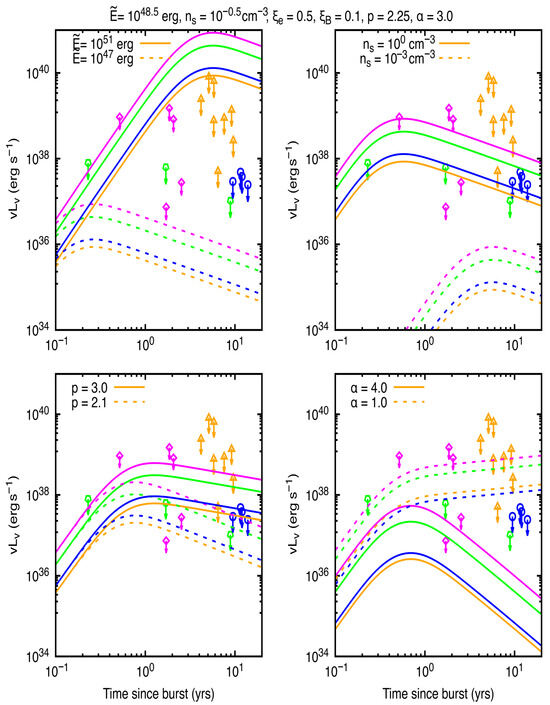
Figure 8.
Radio upper limits ligthcurves from several GRBs reported in the literature. In blue circles corresponds to 3.0 GHz, in magenta diamonds 2.1 GHz, in orange triangles corresponds to 6 GHz and finally in green pentagons corresponds to the 1.4 GHz band. The lightcurves were obtained applying the parameters reported in the header of the figure, and each panel shows two theoretical lightcurves (one solid and the other one dashed) considering variation of one specific parameter on the model, but keeping the others fixed. The data was taken from Fong et al. [173] (orange), Horesh et al. [174] (green), Metzger and Bower [3] (magenta) and Ricci et al. [175] (blue).
The variation is with respect to , , p, and for each panel, starting from the upper left and proceeding in a clockwise direction. All other parameters are predetermined and specified in the header of the figure. In each panel, two theoretical curves (solid and dashed lines) are depicted that vary a single parameter. Specifically, we consider energy (upper left), circumburst number density (upper right), electron spectral index p (lower left) or velocity structure index (lower right). We maintain the other parameters according to the label in the figure. In general, we observe that the dashed lines align more effectively with the upper limits in the majority of panels, while the solid curves are preferred in the lower right panel. In reality, this panel suggests a preference for high values, which result in a more rapid decay of the flux at late periods. In contrast, the slope of the light curve is influenced by the variations in p in the lower left panel, with smaller values resulting in faster declines. The flux density is shifted in the upper panels, while the temporal decay index of the PL is preserved, despite alterations to or . This does not alter the contour of the light curve.
The illustration underscores the degeneracy in parameter space that remains compliant with observational restrictions. Numerous combinations of , p, , and provide valid light curves. This degeneracy demonstrates the difficulty of uniquely identifying the physical parameters of the ejecta or surroundings without further data, such as spectral information, polarization studies, or multi-epoch observations across a wider frequency spectrum.
Figure 9 shows the 3D parameter space for GRB 050906, GRB 080121 and GRB 100216A as a function of the parameters , and . In the particular case of GRB 050906 (left-upper panel), we see that the limitations are the most rigorous within our sample. In reality, the space remains unconstrained only for and . In contrast, at substantial levels of the microphysical parameters, this GRB requires subrelativistic velocities of . In contrast, GRB 080121 (middle panel) has the most limited parameter space. The uncolored area predominates on the graph, indicating that for the majority of and values, the simulated flow consistently remains below the upper limits of the observation, regardless of . Only the upper right corner, representing the most critical microphysical characteristics, has certain limitations. The limits remain rather lenient with , which continues to align with a relativistic shock. The lower panel shows the parameter space of GRB 100216A. This panel shows that these parameters are fully reduced. For instance, lies in 1 × 10⁻¹∼ 7 × 10⁻¹, while for lies in 6 × 10⁻² to 4 × 10⁻¹.
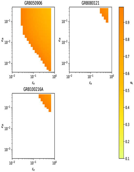
Figure 9.
The parameter space of the rejected values for GRB 050906, GRB 080121 and GRB 100216A. We consider the parameters ranging , and and for a fixed values , , and .
6. Conclusions
- Key outputs and novelty
- We introduce a compact analytic closure for magnetar-field reemergence, encapsulated by a single growth law that reduces crustal microphysics to three observable parameters.
- Closed-form expressions for , , and feed directly into a synchrotron afterglow model, linking internal magnetar evolution to jet-scale energetics without additional nuisance parameters.
- Our framework self-consistently reproduces the timing, flux level, and spectral slope of late-time (–day) cm–mm “bumps”, while remaining agnostic about early X-ray behavior.
- Compared to models without magnetic burial, we obtain order-of-magnitude improvements at day with the addition of only one extra parameter ().
- Constraints from broadband fits (1–100 GHz)
- Emergence timescale: yr; the lower end is Hall–dominated for G, the upper end reflects Ohmic drift at more typical magnetar fields.
- Burial fraction: initial submergence of of the external dipole (), consistent with fallback masses .
- Rebuilt surface field and power: – G and erg s−1, sufficient to account for the observed rebrightenings.
- Robustness: varying the neutron star moment of inertia within modern EoS bounds rescales but shifts by .
- Applications and scope
- We extend the sub-relativistic (deep Newtonian) afterglow formulation of [85], generating light curves when and applying the model to late radio data at 2.1, 1.4, and 6 GHz.
- The parameter space of GRB 050906, GRB 080121, and GRB 100216A is constrained within this unified framework, connecting radio bumps to internal field revival and ejecta–ISM interaction.
- Forecasts: SKA and ngVLA will detect events analogous to at least , offering a decisive test of the buried–magnetar scenario via year-scale, broadly achromatic radio rebrightenings.
- Scope and geometry: should be interpreted as an effective dipolar reemergence timescale. Under strongly hypercritical fallback, the burial outcome is largely insensitive to the seed topology–uniform horizontal/vertical fields, vertical gradients, or loop-like structures–so higher-order multipoles and toroidal flux are phenomenologically absorbed in .
- Microphysics and uncertainties: The effective emergence timescale encapsulates the coupled Hall–Ohm evolution along the cooling history via : cooling lengthens the Ohmic timescale, whereas a higher impurity content (larger ) shortens it. Accordingly, our fits constrain an observationally calibrated , with residual degeneracies against that broadband monitoring, together with VLBI and, when available, polarimetry, can help break.
- Separable coupling and parsimony: We assume a constant coupling efficiency , so the delay kernel alone sets the rebrightening shape and timescale; slow drifts would primarily renormalize the amplitude and leave nearly unchanged at current precision. Our model, therefore, introduces only one physical parameter () relative to no-burial scenarios while delivering order-of-magnitude improvements in fit quality at days, mitigating overfitting concerns.
- Outlook: leveraging source-side delays for future work
The causal, source-side delay introduced here—encoding magnetic burial, Hall–Ohm diffusion, and crustal reconnection via —opens several directions:
- Population inference: Applying the same closure to a nearby controlled GRB sample will yield empirical distributions of and their covariances with the environment () and energetics. This enables testing whether clusters by progenitor channel (collapsars versus mergers) and whether scales with inferred fallback mass.
- Model discrimination: The delay kernel scenario predicts broadly achromatic, year-scale cm–mm bumps with nearly unchanged optically thin spectral index and a single-emergence timescale . This can be contrasted against alternatives (density jumps, refreshed shocks, prolonged fallback without burial), which generically imprint different spectral/temporal couplings and multi-timescale structure. A uniform analysis across events will separate these cases.
- Joint multi-band and imaging tests: Combining 1–100 GHz light curves with VLBI size measurements and late-time calorimetry can break degeneracies between and , anchoring the sub-relativistic dynamics during the deep Newtonian phase. Broadband fits that track the synchrotron peak/SSA evolution provide an internal consistency check of the kernel-driven energy injection.
- Polarization and magnetization probes: If field reemergence drives PWN-like magnetization in the ejecta, low-to-moderate radio linear polarization and modest Faraday rotation trends may appear around (evidencia limitada). Polarimetric monitoring offers an orthogonal test of the mechanism.
- Multi-messenger and context: For mergers that leave long-lived remnants, combining our radio-delay inferences with kilonova ejecta constraints can link to remnant lifetime and composition. In collapsars with SN associations, correlations between and late-time nebular diagnostics (e.g., 56Ni yield) can be explored.
- Forecasts and surveys: The framework yields concrete predictions for detectability with next-generation facilities (e.g., SKA, ngVLA): year-scale, broadly achromatic rebrightenings out to at least the nearby Universe, enabling decisive population tests through regular (monthly) cadence programs.
- Open tools: Releasing the inference pipeline (priors, likelihoods, samplers) and synthetic benchmarks will facilitate reproducibility and enlarge the event pool analyzed under a common delay-kernel framework.
Summary—Source-side delays driven by magnetic burial and Hall–Ohm reemergence provide a minimal, predictive bridge between magnetar microphysics and late-time radio afterglows: a single emergence timescale, , captures both flux normalization and spectral evolution, and yields falsifiable forecasts—year-scale, broadly achromatic cm–mm rebrightenings–testable with uniform 1–100 GHz monitoring, VLBI/polarimetry, and population inference (e.g., SKA/ngVLA).
Author Contributions
Conceptualization: N.F. and C.G.B.; Methodology: N.F. and C.G.B.; Software: A.G. and C.G.B.; Validation: N.F., C.G.B., A.G., B.B.K. and M.G.D.; Writing: N.F., C.G.B., A.G., B.B.K. and M.G.D. All authors have read and agreed to the published version of the manuscript.
Funding
NF is grateful to UNAM-DGAPA-PAPIIT for the funding provided by grant IN112525. AG was supported by Universidad Nacional Autónoma de México Postdoctoral Program (POSDOC). BBK is supported by IBS under the project code IBS-R018-D3. M.G.D. acknowledges funding from the AAS Chretienne Fellowship and the MINIATURA2 grant. The software used in this work was developed in part by the DOE NNSA- and DOE Office of Science-supported Flash Center for Computational Science at the University of Chicago and the University of Rochester.
Data Availability Statement
The data underlying this article will be shared on reasonable request to the corresponding author.
Conflicts of Interest
The authors declare no conflicts of interest.
References
- Kumar, P.; Zhang, B. The physics of gamma-ray bursts & relativistic jets. Phys. Rep. 2015, 561, 1–109. [Google Scholar] [CrossRef]
- Piran, T. Gamma-ray bursts and the fireball model. Phys. Rep. 1999, 314, 575–667. [Google Scholar] [CrossRef]
- Metzger, B.D.; Bower, G.C. Constraints on long-lived remnants of neutron star binary mergers from late-time radio observations of short duration gamma-ray bursts. Mon. Not. R. Astron. Soc. 2014, 437, 1821–1827. [Google Scholar] [CrossRef]
- Duncan, R.C.; Thompson, C. Formation of Very Strongly Magnetized Neutron Stars: Implications for Gamma-Ray Bursts. Astrophys. J. Lett. 1992, 392, L9. [Google Scholar] [CrossRef]
- Usov, V.V. Millisecond pulsars with extremely strong magnetic fields as a cosmological source of gamma-ray bursts. Nature 1992, 357, 472–474. [Google Scholar] [CrossRef]
- Thompson, C. A Model of Gamma-Ray Bursts. Mon. Not. R. Astron. Soc. 1994, 270, 480. [Google Scholar] [CrossRef]
- Metzger, B.; Giannios, D.; Thompson, T.; Bucciantini, N.; Quataert, E. The protomagnetar model for gamma-ray bursts. Mon. Not. R. Astron. Soc. 2011, 413, 2031–2056. [Google Scholar] [CrossRef]
- Woosley, S.E. Gamma-Ray Bursts from Stellar Mass Accretion Disks around Black Holes. Astrophys. J. 1993, 405, 273. [Google Scholar] [CrossRef]
- Paczyński, B. Are Gamma-Ray Bursts in Star-Forming Regions? Astrophys. J. Lett. 1998, 494, L45–L48. [Google Scholar] [CrossRef]
- Woosley, S.E.; Bloom, J.S. The Supernova Gamma-Ray Burst Connection. Annu. Rev. Astron. Astrophys. 2006, 44, 507–556. [Google Scholar] [CrossRef]
- MacFadyen, A.I.; Woosley, S.E. Collapsars: Gamma-Ray Bursts and Explosions in “Failed Supernovae”. Astrophys. J. 1999, 524, 262–289. [Google Scholar] [CrossRef]
- Narayan, R.; Paczynski, B.; Piran, T. Gamma-ray bursts as the death throes of massive binary stars. Astrophys. J. Lett. 1992, 395, L83–L86. [Google Scholar] [CrossRef]
- Fryer, C.L.; Woosley, S.E.; Hartmann, D.H. Formation Rates of Black Hole Accretion Disk Gamma-Ray Bursts. Astrophys. J. 1999, 526, 152–177. [Google Scholar] [CrossRef]
- Barkov, M.V.; Komissarov, S.S. Stellar explosions powered by the Blandford-Znajek mechanism. Mon. Not. R. Astron. Soc. 2008, 385, L28–L32. [Google Scholar] [CrossRef]
- Woosley, S.E.; Heger, A. Long Gamma-Ray Transients from Collapsars. Astrophys. J. 2012, 752, 32. [Google Scholar] [CrossRef]
- Chevalier, R.A. Neutron star accretion in a supernova. Astrophys. J. 1989, 346, 847–859. [Google Scholar] [CrossRef]
- Quataert, E.; Kasen, D. Swift 1644+ 57: The longest gamma-ray burst? Mon. Not. R. Astron. Soc. Lett. 2012, 419, L1–L5. [Google Scholar] [CrossRef]
- Piro, A.L.; Ott, C.D. Supernova fallback onto magnetars and propeller-powered supernovae. Astrophys. J. 2011, 736, 108. [Google Scholar] [CrossRef]
- Rowlinson, A.; O’Brien, P.T.; Tanvir, N.R.; Zhang, B.; Evans, P.A.; Lyons, N.; Levan, A.J.; Willingale, R.; Page, K.L.; Onal, O.; et al. The unusual X-ray emission of the short Swift GRB 090515: Evidence for the formation of a magnetar? Mon. Not. R. Astron. Soc. 2010, 409, 531–540. [Google Scholar] [CrossRef]
- Meszaros, P.; Rees, M.J. Gamma-Ray Bursts: Multiwaveband Spectral Predictions for Blast Wave Models. Astrophys. J. Lett. 1993, 418, L59. [Google Scholar] [CrossRef]
- Panaitescu, A.; Kumar, P. Properties of Relativistic Jets in Gamma-Ray Burst Afterglows. Astrophys. J. 2002, 571, 779–789. [Google Scholar] [CrossRef]
- Taylor, G.B.; Frail, D.A.; Berger, E.; Kulkarni, S.R. The Angular Size and Proper Motion of the Afterglow of GRB 030329. Astrophys. J. Lett. 2004, 609, L1–L4. [Google Scholar] [CrossRef]
- Cavallo, G.; Rees, M.J. A qualitative study of cosmic fireballs and gamma -ray bursts. Mon. Not. R. Astron. Soc. 1978, 183, 359–365. [Google Scholar] [CrossRef]
- Waxman, E. Angular Size and Emission Timescales of Relativistic Fireballs. Astrophys. J. Lett. 1997, 491, L19–L22. [Google Scholar] [CrossRef]
- Fraija, N.; Dainotti, M.G.; Betancourt Kamenetskaia, B.; Galván-Gámez, A.; Aguilar-Ruiz, E. Microphysical parameter variation in gamma-ray burst stratified afterglows and closure relations: From sub-GeV to TeV observations. Mon. Not. R. Astron. Soc. 2024, 527, 1884–1909. [Google Scholar] [CrossRef]
- Fraija, N.; Kamenetskaia, B.B.; Gámez, A.G.; Dainotti, M.G.; Vargas, H.L. Closure Relations of Synchrotron Self-Compton from Reverse shock and Fermi-LAT GRBs. Mon. Not. R. Astron. Soc. 2025, 543, 1945–1973. [Google Scholar] [CrossRef]
- Fraija, N.; Betancourt Kamenetskaia, B.; Galván-Gámez, A.; Veres, P.; Becerra, R.L.; Dichiara, S.; Dainotti, M.G.; Lizcano, F.; Aguilar-Ruiz, E. An explanation of GRB Fermi-LAT flares and high-energy photons in stratified afterglows. Mon. Not. R. Astron. Soc. 2024, 527, 1674–1704. [Google Scholar] [CrossRef]
- Sari, R.; Mészáros, P. Impulsive and Varying Injection in Gamma-Ray Burst Afterglows. Astrophys. J. Lett. 2000, 535, L33–L37. [Google Scholar] [CrossRef] [PubMed]
- Nakar, E.; Piran, T.; Granot, J. Variability in GRB Afterglows and GRB 021004. New Astron. 2003, 8, 495–505. [Google Scholar] [CrossRef][Green Version]
- Uhm, Z.L.; Beloborodov, A.M. On the Mechanism of Gamma-Ray Burst Afterglows. Astrophys. J. Lett. 2007, 665, L93–L96. [Google Scholar] [CrossRef]
- Rossi, E.; Lazzati, D.; Rees, M.J. Afterglow Light Curves, Viewing Angle and the Jet Structure of γ-ray Bursts. Mon. Not. R. Astron. Soc. 2002, 332, 945–950. [Google Scholar] [CrossRef]
- Ryan, G.; van Eerten, H.; MacFadyen, A.; Zhang, B.B. Gamma-Ray Bursts Are Observed Off-axis. Astrophys. J. 2015, 799, 3. [Google Scholar] [CrossRef]
- Fraija, N.; Galvan-Gamez, A.; Betancourt Kamenetskaia, B.; Dainotti, M.G.; Dichiara, S.; Veres, P.; Becerra, R.L.; do E., S. Pedreira, A.C.C. Modeling Gamma-Ray Burst Afterglow Observations with an Off-axis Jet Emission. Astrophys. J. 2022, 940, 189. [Google Scholar] [CrossRef]
- Fraija, N.; Dainotti, M.G.; Levine, D.; Kamenetskaia, B.B.; Galvan-Gamez, A. Off-axis Afterglow Closure Relations and Fermi-LAT Detected Gamma-Ray Bursts. Astrophys. J. 2023, 958, 126. [Google Scholar] [CrossRef]
- Fraija, N.; Kamenetskaia, B.B.; Galván, A.; Montalvo, A.; Do E S Pedreira, A.C.C.; Veres, P.; Becerra, R.L.; Dainotti, M.G.; Dichiara, S.; Vargas, H.L. Late-afterglow Emission from a Quasi-spherical Outflow in a stratified environment. Mon. Not. R. Astron. Soc. 2025. [Google Scholar] [CrossRef]
- Granot, J.; Königl, A.; Piran, T. Implications of the early X-ray afterglow light curves of Swift gamma-ray bursts. Mon. Not. R. Astron. Soc. 2006, 370, 1946–1960. [Google Scholar] [CrossRef]
- Thompson, C.; Duncan, R.C. Neutron Star Dynamos and the Origins of Pulsar Magnetism. Astrophys. J. 1993, 408, 194. [Google Scholar] [CrossRef]
- Geppert, U.; Page, D.; Zannias, T. Central compact objects in supernova remnants. Astron. Astrophys. 1999, 345, 847–854. [Google Scholar]
- Choudhuri, A.R.; Konar, S. Diamagnetic screening of the magnetic field in accreting neutron stars. Mon. Not. R. Astron. Soc. 2002, 332, 933–944. [Google Scholar] [CrossRef][Green Version]
- Michel, F.C. Magnetic structure of pulsar winds. Astrophys. J. 1994, 431, 397–401. [Google Scholar] [CrossRef]
- Muslimov, A.; Page, D. Magnetic and spin history of very young pulsars. Astrophys. J. 1995, 458, 347. [Google Scholar] [CrossRef]
- Konar, S. Magnetic fields of neutron stars. J. Astrophys. Astron. 2017, 38, 47. [Google Scholar] [CrossRef]
- Vigelius, M.; Melatos, A. Resistive relaxation of a magnetically confined mountain on an accreting neutron star. Mon. Not. R. Astron. Soc. 2009, 395, 1985–1998. [Google Scholar] [CrossRef]
- Li, S.; Beloborodov, A.M. Plastic flow of a neutron star crust mediated by electron captures. Astrophys. J. 2015, 815, 25. [Google Scholar] [CrossRef]
- Gourgouliatos, K.; Cumming, A. Hall effect in neutron star crusts: Evolution, endpoint and dependence on initial conditions. Mon. Not. R. Astron. Soc. 2014, 438, 1618–1629. [Google Scholar] [CrossRef]
- Bernal, C.G.; Page, D.; Lee, W.H. ypercritical accretion onto a newborn neutron star and magnetic field submergence. Astrophys. J. 2013, 770, 106. [Google Scholar] [CrossRef]
- Kasen, D.; Bildsten, L. Supernova Light Curves Powered by Young Magnetars. Astrophys. J. 2010, 717, 245–249. [Google Scholar] [CrossRef]
- Metzger, B.D.; Piro, A.L. Optical and X-ray emission from stable millisecond magnetars formed from the merger of binary neutron stars. Mon. Not. R. Astron. Soc. 2014, 439, 3916–3930. [Google Scholar] [CrossRef]
- Metzger, B.D. Kilonovae. Living Rev. Relativ. 2019, 23, 1. [Google Scholar] [CrossRef]
- Amelino-Camelia, G.; Ellis, J.; Mavromatos, N.E.; Nanopoulos, D.V.; Sarkar, S. Tests of quantum gravity from observations of γ-ray bursts. Nature 1998, 393, 763–765. [Google Scholar] [CrossRef]
- Vasileiou, V.; Jacholkowska, A.; Piron, F.; Bolmont, J.; Couturier, C.; Granot, J.; Stecker, F.W.; Cohen-Tanugi, J.; Longo, F. Constraints on Lorentz invariance violation from Fermi-Large Area Telescope observations of gamma-ray bursts. Phys. Rev. D 2013, 87, 122001. [Google Scholar] [CrossRef]
- Acciari, V.A.; MAGIC Collaboration. Bounds on Lorentz Invariance Violation from MAGIC Observation of GRB 190114C. Phys. Rev. Lett. 2020, 125, 021301. [Google Scholar] [CrossRef] [PubMed]
- Piran, T.; Ofengeim, D.D. Lorentz invariance violation limits from GRB 221009A. Phys. Rev. D 2024, 109, L081501. [Google Scholar] [CrossRef]
- Bernal, C.G.; Lee, W.H.; Page, D. Hypercritical accretion onto a magnetized neutron star surface: A numerical approach. arXiv 2010, arXiv:1006.3003. [Google Scholar] [CrossRef]
- Fraija, N.; Bernal, C.G. Hypercritical accretion phase and neutrino expectation in the evolution of Cassiopeia A. Mon. Not. R. Astron. Soc. 2015, 451, 455–466. [Google Scholar] [CrossRef]
- Viganò, D.; Pons, J.A. Central compact objects and the hidden magnetic field scenario. Mon. Not. R. Astron. Soc. 2012, 425, 2487–2492. [Google Scholar] [CrossRef]
- Fryxell, B.; Olson, K.; Ricker, P.; Timmes, F.X.; Zingale, M.; Lamb, D.; MacNeice, P.; Rosner, R.; Truran, J.; Tufo, H. FLASH: An adaptive mesh hydrodynamics code for modeling astrophysical thermonuclear flashes. Astrophys. J. Suppl. Ser. 2000, 131, 273. [Google Scholar] [CrossRef]
- Haskell, B.; Samuelsson, L.; Glampedakis, K.; Andersson, N. Modelling magnetically deformed neutron stars. Mon. Not. R. Astron. Soc. 2008, 385, 531–542. [Google Scholar] [CrossRef]
- Mukherjee, D. Revisiting field burial by accretion onto neutron stars. J. Astrophys. Astron. 2017, 38, 48. [Google Scholar] [CrossRef]
- Chevalier, R.A.; Emmering, R.T. Are pulsars born as slow rotators? Astrophys. J. 1986, 304, 140–153. [Google Scholar] [CrossRef]
- Perna, R.; Pons, J.A. A Unified Model of the Magnetar and Radio Pulsar Bursting Phenomenology. Astrophys. J. Lett. 2011, 727. [Google Scholar] [CrossRef]
- Goldreich, P.; Reisenegger, A. Magnetic Field Decay in Isolated Neutron Stars. Astrophys. J. 1992, 395, 250–258. [Google Scholar] [CrossRef]
- Potekhin, A.Y.; Pons, J.A.; Page, D. Neutron Stars—Cooling and Transport. Space Sci. Rev. 2015, 191, 239–291. [Google Scholar] [CrossRef]
- Cumming, A.; Arras, P.; Zweibel, E. Magnetic field evolution in neutron star crusts due to the Hall effect and ohmic decay. Astrophys. J. 2004, 609, 999. [Google Scholar] [CrossRef]
- Shalybkov, D.; Urpin, V. Ambipolar diffusion and anisotropy of resistivity in neutron star cores. Mon. Not. R. Astron. Soc. 1995, 273, 643–648. [Google Scholar] [CrossRef]
- Skiathas, D.; Gourgouliatos, K.N. Combined magnetic field evolution in neutron star cores and crusts: Ambipolar diffusion, Hall effect, and Ohmic dissipation. Mon. Not. R. Astron. Soc. 2024, 528, 5178–5188. [Google Scholar] [CrossRef]
- Pons, J.A.; Geppert, U. Magnetic field dissipation in neutron star crusts: From magnetars to isolated neutron stars. Astron. Astrophys. 2007, 470, 303–315. [Google Scholar] [CrossRef]
- Kojima, Y.; Kisaka, S. Magnetic field decay with Hall drift in neutron star crusts. Mon. Not. R. Astron. Soc. 2012, 421, 2722–2730. [Google Scholar] [CrossRef]
- Chamel, N.; Haensel, P. Physics of neutron star crusts. Living Rev. Relativ. 2008, 11, 10. [Google Scholar] [CrossRef]
- Ho, W.C. Evolution of a buried magnetic field in the central compact object neutron stars. Mon. Not. R. Astron. Soc. 2011, 414, 2567–2575. [Google Scholar] [CrossRef]
- Yakovlev, D.; Kaminker, A.; Gnedin, O.Y.; Haensel, P. Neutrino emission from neutron stars. Phys. Rep. 2001, 354, 1–155. [Google Scholar] [CrossRef]
- Aguilera, D.N.; Pons, J.A.; Miralles, J.A. 2D cooling of magnetised neutron stars. Astron. Astrophys. 2008, 486, 255–271. [Google Scholar] [CrossRef]
- Viganò, D.; Rea, N.; Pons, J.A.; Perna, R.; Aguilera, D.N.; Miralles, J.A. Unifying the observational diversity of isolated neutron stars via magneto-thermal evolution models. Mon. Not. R. Astron. Soc. 2013, 434, 123–141. [Google Scholar] [CrossRef]
- Lyutikov, M. Magnetar activity mediated by plastic deformations of neutron star crust. Mon. Not. R. Astron. Soc. 2015, 447, 1407–1417. [Google Scholar] [CrossRef]
- Lander, S.K. Magnetar Field Evolution and Crustal Plasticity. Astrophys. J. Lett. 2016, 824, L21. [Google Scholar] [CrossRef]
- Levin, Y.; Lyutikov, M. On the dynamics of mechanical failures in magnetized neutron star crusts. Mon. Not. R. Astron. Soc. 2012, 427, 1574–1579. [Google Scholar] [CrossRef]
- Chugunov, A.I.; Horowitz, C.J. Breaking stress of neutron star crust. Mon. Not. R. Astron. Soc. Lett. 2010, 407, L54–L58. [Google Scholar] [CrossRef]
- Li, X.; Beloborodov, A.M. Plastic damping of alfvén waves in magnetar flares and delayed afterglow emission. Astrophys. J. 2015, 815, 25. [Google Scholar] [CrossRef]
- Fraija, N.; Bernal, C.; Morales, G.; Negreiros, R. Hypercritical accretion scenario in central compact objects accompanied with an expected neutrino burst. Phys. Rev. D 2018, 98, 083012. [Google Scholar] [CrossRef]
- Metzger, B.; Beniamini, P.; Giannios, D. Effects of Fallback Accretion on Protomagnetar Outflows in Gamma-Ray Bursts and Superluminous Supernovae. Astrophys. J. 2018, 857. [Google Scholar] [CrossRef]
- Suvorov, A.G.; Melatos, A. Recycled pulsars with multipolar magnetospheres from accretion-induced magnetic burial. Mon. Not. R. Astron. Soc. 2020, 499, 3243–3254. [Google Scholar] [CrossRef]
- Troja, E.; Piro, L.; Eerten, H.; Wollaeger, R.T.; Im, M.; Fox, O.D.; Butler, N.R.; Cenko, S.B.; Sakamoto, T.; Fryer, C.L.; et al. The X-ray counterpart to the gravitational-wave event GW170817. Nature 2017, 551, 71–74. [Google Scholar] [CrossRef]
- Hajela, A.; Margutti, R.; Bright, J.; Alexander, K.; Metzger, B.; Nedora, V.; Kathirgamaraju, A.; Margalit, B.; Radice, D.; Guidorzi, C.; et al. Evidence for X-ray emission in excess to the jet-afterglow decay 3.5 yr after the binary neutron star merger GW 170817: A new emission component. Astrophys. J. Lett. 2022, 927, L17. [Google Scholar] [CrossRef]
- Bernal, C.G.; Frajuca, C.; Hirsch, H.D.; Minari, B.; Magalhaes, N.S.; Selbach, L.B. On the overall properties of young neutron stars: An application to the Crab pulsar. Front. Astron. Space Sci. 2024, 11, 1390597. [Google Scholar] [CrossRef]
- Fraija, N.; Bernal, C.G.; Galván-Gámez, A.; Kamenetskaia, B.B.; Dainotti, M.G. Magnetic burial in millisecond magnetars and late GRB afterglow signatures. Mon. Not. R. Astron. Soc. 2025, 541, 1487–1506. [Google Scholar] [CrossRef]
- Tan, J.C.; Matzner, C.D.; McKee, C.F. Trans-Relativistic Blast Waves in Supernovae as Gamma-Ray Burst Progenitors. Astrophys. J. 2001, 551, 946–972. [Google Scholar] [CrossRef]
- Grossman, D.; Korobkin, O.; Rosswog, S.; Piran, T. The long-term evolution of neutron star merger remnants - II. Radioactively powered transients. Mon. Not. R. Astron. Soc. 2014, 439, 757–770. [Google Scholar] [CrossRef]
- Rowlinson, A.; O’brien, P.; Metzger, B.; Tanvir, N.; Levan, A.J. Signatures of magnetar central engines in short GRB light curves. Mon. Not. R. Astron. Soc. 2013, 430, 1061–1087. [Google Scholar] [CrossRef]
- Bernardini, M.; Campana, S.; Ghisellini, G.; d’Avanzo, P.; Burlon, D.; Covino, S.; Ghirlanda, G.; Melandri, A.; Salvaterra, R.; Vergani, S.; et al. How to switch a gamma-ray burst on and off through a magnetar. Astrophys. J. 2013, 775, 67. [Google Scholar] [CrossRef]
- Fraija, N.; Bernal, C.G.; Hidalgo-Gamez, A.M. Signatures of neutrino cooling in the SN1987A scenario. Mon. Not. R. Astron. Soc. 2014, 442, 239–250. [Google Scholar] [CrossRef][Green Version]
- Dai, Z.G.; Cheng, K.S. Afterglow Emission from Highly Collimated Jets with Flat Electron Spectra: Application to the GRB 010222 Case? Astrophys. J. Lett. 2001, 558, L109–L112. [Google Scholar] [CrossRef]
- Fraija, N.; Dainotti, M.G.; Kamenetskaia, B.B.; Levine, D.; Galvan-Gamez, A. Closure relations of synchrotron self-compton in afterglow-stratified medium and Fermi-LAT detected gamma-ray bursts. Mon. Not. R. Astron. Soc. 2023, 525, 1630–1640. [Google Scholar] [CrossRef]
- Fraija, N.; Dainotti, M.G.; Ugale, S.; Jyoti, D.; Warren, D.C. Synchrotron Self-Compton Afterglow Closure Relations and Fermi-LAT-detected Gamma-Ray Bursts. Astrophys. J. 2022, 934, 188. [Google Scholar] [CrossRef]
- Chevalier, R.A.; Li, Z.Y. Wind Interaction Models for Gamma-Ray Burst Afterglows: The Case for Two Types of Progenitors. Astrophys. J. 2000, 536, 195–212. [Google Scholar] [CrossRef]
- Panaitescu, A.; Mészáros, P. Radiative Regimes in Gamma-Ray Bursts and Afterglows. Astrophys. J. 1998, 501, 772–779. [Google Scholar] [CrossRef]
- Tak, D.; Omodei, N.; Uhm, Z.L.; Racusin, J.; Asano, K.; McEnery, J. Closure Relations of Gamma-Ray Bursts in High Energy Emission. Astrophys. J. 2019, 883, 134. [Google Scholar] [CrossRef]
- Dainotti, M.G.; Omodei, N.; Srinivasaragavan, G.P.; Vianello, G.; Willingale, R.; O’Brien, P.; Nagataki, S.; Petrosian, V.; Nuygen, Z.; Hernandez, X.; et al. On the Existence of the Plateau Emission in High-energy Gamma-Ray Burst Light Curves Observed by Fermi-LAT. Astrophys. J. Suppl. Ser. 2021, 255, 13. [Google Scholar] [CrossRef]
- Dainotti, M.; Levine, D.; Fraija, N.; Warren, D.; Veres, P.; Sourav, S. The Closure Relations in High-Energy Gamma-ray Bursts Detected by Fermi-LAT. Galaxies 2023, 11, 25. [Google Scholar] [CrossRef]
- Ajello, M.; Arimoto, M.; Axelsson, M.; Baldini, L.; Barbiellini, G.; Bastieri, D.; Bellazzini, R.; Bhat, P.N.; Bissaldi, E.; Blandford, R.D.; et al. A Decade of Gamma-Ray Bursts Observed by Fermi-LAT: The Second GRB Catalog. Astrophys. J. 2019, 878, 52. [Google Scholar] [CrossRef]
- Racusin, J.L.; Liang, E.W.; Burrows, D.N.; Falcone, A.; Sakamoto, T.; Zhang, B.B.; Zhang, B.; Evans, P.; Osborne, J. Jet Breaks and Energetics of Swift Gamma-Ray Burst X-Ray Afterglows. Astrophys. J. 2009, 698, 43–74. [Google Scholar] [CrossRef]
- Srinivasaragavan, G.P.; Dainotti, M.G.; Fraija, N.; Hernandez, X.; Nagataki, S.; Lenart, A.; Bowden, L.; Wagner, R. On the Investigation of the Closure Relations for Gamma-Ray Bursts Observed by Swift in the Post-plateau Phase and the GRB Fundamental Plane. Astrophys. J. 2020, 903, 18. [Google Scholar] [CrossRef]
- Dainotti, M.G.; Lenart, A.Ł.; Fraija, N.; Nagataki, S.; Warren, D.C.; De Simone, B.; Srinivasaragavan, G.; Mata, A. Closure relations during the plateau emission of Swift GRBs and the fundamental plane. Publ. Astron. Soc. Jpn. 2021, 73, 970–1000. [Google Scholar] [CrossRef]
- Oates, S.R.; Page, M.J.; De Pasquale, M.; Schady, P.; Breeveld, A.A.; Holland, S.T.; Kuin, N.P.M.; Marshall, F.E. A correlation between the intrinsic brightness and average decay rate of Swift/UVOT gamma-ray burst optical/ultraviolet light curves. Mon. Not. R. Astron. Soc. 2012, 426, L86–L90. [Google Scholar] [CrossRef]
- Yost, S.A.; Harrison, F.A.; Sari, R.; Frail, D.A. A Study of the Afterglows of Four Gamma-Ray Bursts: Constraining the Explosion and Fireball Model. Astrophys. J. 2003, 597, 459–473. [Google Scholar] [CrossRef]
- Kumar, P.; Panaitescu, A. A unified treatment of the gamma-ray burst 021211 and its afterglow. Mon. Not. R. Astron. Soc. 2003, 346, 905–914. [Google Scholar] [CrossRef]
- Ioka, K.; Toma, K.; Yamazaki, R.; Nakamura, T. Efficiency crisis of swift gamma-ray bursts with shallow X-ray afterglows: Prior activity or time-dependent microphysics? A&A 2006, 458, 7–12. [Google Scholar] [CrossRef]
- Fan, Y.; Piran, T. Gamma-ray burst efficiency and possible physical processes shaping the early afterglow. Mon. Not. R. Astron. Soc. 2006, 369, 197–206. [Google Scholar] [CrossRef]
- Panaitescu, A.; Mészáros, P.; Burrows, D.; Nousek, J.; Gehrels, N.; O’Brien, P.; Willingale, R. Evidence for chromatic X-ray light-curve breaks in Swift gamma-ray burst afterglows and their theoretical implications. Mon. Not. R. Astron. Soc. 2006, 369, 2059–2064. [Google Scholar] [CrossRef]
- Ioka, K. Coherent Radiation in Gamma-Ray Bursts and Relativistic Collisionless Shocks. Prog. Theor. Phys. 2005, 114, 1317–1322. [Google Scholar] [CrossRef][Green Version]
- Lemoine, M. Synchrotron signature of a relativistic blast wave with decaying microturbulence. Mon. Not. R. Astron. Soc. 2013, 428, 845–866. [Google Scholar] [CrossRef][Green Version]
- Fraija, N.; Laskar, T.; Dichiara, S.; Beniamini, P.; Duran, R.B.; Dainotti, M.G.; Becerra, R.L. GRB Fermi-LAT Afterglows: Explaining Flares, Breaks, and Energetic Photons. Astrophys. J. 2020, 905, 112. [Google Scholar] [CrossRef]
- Kong, S.W.; Wong, A.Y.L.; Huang, Y.F.; Cheng, K.S. Variation of microphysics in wind bubbles: An alternative mechanism for explaining the rebrightenings in Gamma-ray burst afterglows. Mon. Not. R. Astron. Soc. 2010, 402, 409–416. [Google Scholar] [CrossRef]
- Dichiara, S.; Troja, E.; O’Connor, B.; Marshall, F.E.; Beniamini, P.; Cannizzo, J.K.; Lien, A.Y.; Sakamoto, T. Short gamma-ray bursts within 200 Mpc. Mon. Not. R. Astron. Soc. 2020, 492, 5011–5022. [Google Scholar] [CrossRef]
- Lien, A.; Sakamoto, T.; Barthelmy, S.D.; Baumgartner, W.H.; Cannizzo, J.K.; Chen, K.; Collins, N.R.; Cummings, J.R.; Gehrels, N.; Krimm, H.A.; et al. The Third Swift Burst Alert Telescope Gamma-Ray Burst Catalog. Astrophys. J. 2016, 829, 7. [Google Scholar] [CrossRef]
- Abac, A.G.; Abbott, R.; Abouelfettouh, I.; Acernese, F.; Ackley, K.; Adhicary, S.; Adhikari, N.; Ligo Scientific Collaboration; VIRGO Collaboration; Kagra Collaboration. Observation of Gravitational Waves from the Coalescence of a 2.5–4.5 M ⊙ Compact Object and a Neutron Star. Astrophys. J. Lett. 2024, 970, L34. [Google Scholar] [CrossRef]
- Roberts, O.; Veres, P.; Baring, M.; Briggs, M.; Kouveliotou, C.; Bissaldi, E.; Younes, G.; Chastain, S.; DeLaunay, J.; Huppenkothen, D.; et al. Rapid spectral variability of a giant flare from a magnetar in NGC 253. Nature 2021, 589, 207–210. [Google Scholar] [CrossRef] [PubMed]
- Gao, H.; Ding, X.H.; Wu, X.; Dai, Z.; Zhang, B. GRB 080503 LATE AFTERGLOW RE-BRIGHTENING: SIGNATURE OF A MAGNETAR-POWERED MERGER-NOVA. Astrophys. J. 2015, 807, 163. [Google Scholar] [CrossRef]
- Lü, H.J.; Zhang, B. A test of the millisecond magnetar central engine model of gamma-ray bursts with swift data. Astrophys. J. 2014, 785, 74. [Google Scholar] [CrossRef]
- Li, L.; Wu, X.F.; Lei, W.H.; Dai, Z.G.; Liang, E.W.; Ryde, F. Constraining the Type of Central Engine of GRBs with Swift Data. Astrophys. J. Suppl. Ser. 2018, 236, 26. [Google Scholar] [CrossRef]
- Hurley, K.; Boggs, S.E.; Smith, D.M.; Duncan, R.C.; Lin, R.; Zoglauer, A.; Krucker, S.; Hurford, G.; Hudson, H.; Wigger, C.; et al. An exceptionally bright flare from SGR 1806-20 and the origins of short-duration γ-ray bursts. Nature 2005, 434, 1098–1103. [Google Scholar] [CrossRef]
- Villasenor, J.S.; Lamb, D.Q.; Ricker, G.R.; Atteia, J.L.; Kawai, N.; Butler, N.; Nakagawa, Y.; Jernigan, J.G.; Boer, M.; Crew, G.B.; et al. Discovery of the short γ-ray burst GRB 050709. Nature 2005, 437, 855–858. [Google Scholar] [CrossRef] [PubMed]
- Butler, N.; Ricker, G.; Atteia, J.L.; Kawai, N.; Lamb, D.; Woosley, S.; Arimoto, M.; Donaghy, T.; Fenimore, E.; Galassi, M.; et al. GRB050709: A possible short-hard GRB localized by HETE. GRB Coord. Netw. 2005, 3570, 1. [Google Scholar]
- Morgan, A.; Grupe, D.; Gronwall, C.; Racusin, J.; Falcone, A.; Marshall, F.; Chester, M.; Gehrels, N. GRB 050709: Swift UVOT and XRT observations. GRB Coord. Netw. 2005, 3577, 1. [Google Scholar]
- Covino, S.; Malesani, D.; Israel, G.L.; D’Avanzo, P.; Antonelli, L.A.; Chincarini, G.; Fugazza, D.; Conciatore, M.L.; Della Valle, M.; Fiore, F.; et al. Optical emission from GRB 050709: A short/hard GRB in a star-forming galaxy. A&A 2006, 447, L5–L8. [Google Scholar] [CrossRef]
- Krimm, H.; Barbier, L.; Barthelmy, S.; Cummings, J.; Fenimore, E.; Gehrels, N.; Hinshaw, D.; Hullinger, D.; Markwardt, C.; McLean, K.; et al. GRB050724: Refined analysis of the Swift-BAT possible short burst. GRB Coord. Netw. 2005, 3667, 1. [Google Scholar]
- Campana, S.; Tagliaferri, G.; Lazzati, D.; Chincarini, G.; Covino, S.; Page, K.; Romano, P.; Moretti, A.; Cusumano, G.; Mangano, V.; et al. The X-ray afterglow of the short gamma ray burst 050724. A&A 2006, 454, 113–117. [Google Scholar] [CrossRef][Green Version]
- Prochaska, J.X.; Bloom, J.S.; Chen, H.W.; Hansen, B.; Kalirai, J.; Rich, M.; Richer, H. GRB 050724: Secure host redshift from Keck. GRB Coord. Netw. 2005, 3700, 1. [Google Scholar]
- Krimm, H.; La Parola, V.; de Pasquale, M.; Barthelmy, S.; Blustin, A.; Burrows, D.; Gehrels, N.; Gronwall, C.; Pagani, C.; Page, K. GRB 050906: Swift/BAT detection of a possible burst. GRB Coord. Netw. 2005, 3926, 1. [Google Scholar]
- Cameron, P.B.; Frail, D.A. GRB 050906. summary of radio observations. GRB Coord. Netw. 2005, 4060, 1. [Google Scholar]
- Levan, A.; Tanvir, N. GRB 050906: Bright galaxy in BAT error box. GRB Coord. Netw. 2005, 3927, 1. [Google Scholar]
- Parsons, A.; Barthelmy, S.; Burrows, D.; Capalbi, M.; Cummings, J.; Gehrels, N.; Gronwall, C.; Krimm, H.; Markwardt, C.; Marshall, F.; et al. GRB 051221: Swift detection of a bright short burst. GRB Coord. Netw. 2005, 4363, 1. [Google Scholar]
- Grupe, D.; Burrows, D.N.; Patel, S. GRB 051221A: Chandra afterglow position. GRB Coord. Netw. 2005, 4389, 1. [Google Scholar]
- Soderberg, A.M.; Berger, E.; Kasliwal, M.; Frail, D.A.; Price, P.A.; Schmidt, B.P.; Kulkarni, S.R.; Fox, D.B.; Cenko, S.B.; Gal-Yam, A.; et al. The Afterglow, Energetics, and Host Galaxy of the Short-Hard Gamma-Ray Burst 051221a. Astrophys. J. 2006, 650, 261–271. [Google Scholar] [CrossRef]
- Barbier, L.; Barthelmy, S.; Beardmore, A.; Burrows, D.; Cummings, J.; Falcone, A.; Gehrels, N.; Page, K.; Retter, A.; Roming, P.; et al. GRB 051227: Swift detection of a burst. GRB Coord. Netw. 2005, 4397, 1. [Google Scholar]
- Beardmore, A.; Burrows, D.N.; Page, K.; Marshall, F.; Chester, M. GRB 051227: XRT refined analysis. GRB Coord. Netw. 2005, 4402, 1. [Google Scholar]
- D’Avanzo, P.; Malesani, D.; Covino, S.; Piranomonte, S.; Grazian, A.; Fugazza, D.; Margutti, R.; D’Elia, V.; Antonelli, L.A.; Campana, S.; et al. The optical afterglows and host galaxies of three short/hard gamma-ray bursts. A&A 2009, 498, 711–721. [Google Scholar] [CrossRef]
- Pagani, C.; Burrows, D. GRB 060313: Swift XRT position. GRB Coord. Netw. 2006, 4870, 1. [Google Scholar]
- Roming, P.W.A.; Vanden Berk, D.; Pal’shin, V.; Pagani, C.; Norris, J.; Kumar, P.; Krimm, H.; Holland, S.T.; Gronwall, C.; Blustin, A.J.; et al. GRB 060313: A New Paradigm for Short-Hard Bursts? Astrophys. J. 2006, 651, 985–993. [Google Scholar] [CrossRef]
- Pagani, C.; Barthelmy, S.; Cummings, J.; Gehrels, N.; Grupe, D.; Holland, S.T.; Hunsberger, S.; Markwardt, C.; Marshall, F.; Palmer, D. GRB 060313: Swift-BAT detection of a bright short hard burst. GRB Coord. Netw. 2006, 4867, 1. [Google Scholar]
- Pagani, C.; Morris, D.; Grupe, D.; Burrows, D. GRB 060313: Swift-XRT team refined analysis. GRB Coord. Netw. 2006, 4875, 1. [Google Scholar]
- Hullinger, D.; Barbier, L.; Barthelmy, S.; Cummings, J.; Fenimore, E.; Gehrels, N.; Krimm, H.; Koss, M.; Markwardt, C.; Palmer, D.; et al. GRB 060505 BAT refined analysis. GRB Coord. Netw. 2006, 5142, 1. [Google Scholar]
- Palmer, D.; Cummings, J.; Stamatikos, M.; Markwardt, C.; Sakamoto, T. GRB 060505: Swift-BAT detection of a weak burst. GRB Coord. Netw. 2006, 5076, 1. [Google Scholar]
- Ofek, E.O.; Cenko, S.B.; Gal-Yam, A.; Fox, D.B.; Nakar, E.; Rau, A.; Frail, D.A.; Kulkarni, S.R.; Price, P.A.; Schmidt, B.P.; et al. GRB 060505: A Possible Short-Duration Gamma-Ray Burst in a Star-forming Region at a Redshift of 0.09. Astrophys. J. 2007, 662, 1129–1135. [Google Scholar] [CrossRef]
- Racusin, J.L.; Barthelmy, S.D.; Burrows, D.N.; Chester, M.M.; Gehrels, N.; Krimm, H.A.; Palmer, D.M.; Sakamoto, T. GRB 070714: Swift detection of a bright burst, possibly short. GRB Coord. Netw. 2006, 6020, 1. [Google Scholar]
- Gao, H.; Zhang, B.; Lü, H.J.; Li, Y. Searching for Magnetar-powered Merger-novae from Short GRBS. Astrophys. J. 2017, 837, 50. [Google Scholar] [CrossRef]
- Graham, J.F.; Fruchter, A.S.; Levan, A.J.; Melandri, A.; Kewley, L.J.; Levesque, E.M.; Nysewander, M.; Tanvir, N.R.; Dahlen, T.; Bersier, D.; et al. GRB 070714B—Discovery of the Highest Spectroscopically Confirmed Short Burst Redshift. Astrophys. J. 2009, 698, 1620–1629. [Google Scholar] [CrossRef]
- Ziaeepour, H.; Barthelmy, S.D.; Parsons, A.; Page, K.L.; de Pasquale, M.; Schady, P. Final Swift observations of GRB 070724A. GCN Rep. 2007, 74, 2. [Google Scholar]
- Berger, E.; Cenko, S.B.; Fox, D.B.; Cucchiara, A. Discovery of the Very Red Near-Infrared and Optical Afterglow of the Short-Duration GRB 070724A. Astrophys. J. 2009, 704, 877–882. [Google Scholar] [CrossRef]
- Berger, E. The Host Galaxies of Short-Duration Gamma-Ray Bursts: Luminosities, Metallicities, and Star-Formation Rates. Astrophys. J. 2009, 690, 231–237. [Google Scholar] [CrossRef]
- Cummings, J.R.; Palmer, D.M. GRB 080121: Swift-BAT detection of a very weak, short burst. GRB Coord. Netw. 2008, 7209, 1. [Google Scholar]
- Troja, E.; Burrows, D.N. GRB 080121: Upper limit on X-ray afterglow. GRB Coord. Netw. 2008, 7224, 1. [Google Scholar]
- Perley, D.A.; Foley, R.J.; Bloom, J.S. GRB 080121: Nearby SDSS galaxies. GRB Coord. Netw. 2008, 7210, 1. [Google Scholar]
- Pagani, C.; Baumgartner, W.H.; Beardmore, A.P.; Chester, M.M.; Cummings, J.R.; Evans, P.A.; Gehrels, N.; Grupe, D.; Holland, S.T.; Krimm, H.A.; et al. GRB 080905: Swift detection of a probably-short burst. GRB Coord. Netw. 2008, 8180, 1. [Google Scholar]
- Cummings, J.; Barthelmy, S.D.; Baumgartner, W.; Fenimore, E.; Gehrels, N.; Krimm, H.; Markwardt, C.; Palmer, D.; Pagani, C.; Sakamoto, T.; et al. RB 080905A, Swift-BAT refined analysis. GRB Coord. Netw. 2008, 8187, 1. [Google Scholar]
- Rowlinson, A.; Wiersema, K.; Levan, A.J.; Tanvir, N.R.; O’Brien, P.T.; Rol, E.; Hjorth, J.; Thöne, C.C.; de Ugarte Postigo, A.; Fynbo, J.P.U.; et al. Discovery of the afterglow and host galaxy of the low-redshift short GRB 080905A. Mon. Not. R. Astron. Soc. 2010, 408, 383–391. [Google Scholar] [CrossRef]
- Guiriec, S.; Connaughton, V.; Briggs, M. GRB 090510: Fermi GBM detection. GRB Coord. Netw. 2009, 9336, 1. [Google Scholar]
- Hoversten, E.A.; Barthelmy, S.D.; Burrows, D.N.; Chester, M.M.; Grupe, D.; Kennea, J.A.; Krimm, H.A.; Kuin, N.P.M.; Palmer, D.M.; Ukwatta, T.N. GRB 090510: Swift detection of a short hard burst. GRB Coord. Netw. 2009, 9331, 1. [Google Scholar]
- Ohno, M.; Pelassa, V. Fermi LAT detection of GRB 090510. GRB Coord. Netw. 2009, 9334, 1. [Google Scholar]
- Rau, A.; McBreen, S.; Kruehler, T.; Greiner, J. GRB090510: VLT/FORS2 spectroscopic redshift. GRB Coord. Netw. 2009, 9353, 1. [Google Scholar]
- Beardmore, A.P.; Kennea, J.A.; Markwardt, C.B.; O’Brien, P.T.; Page, K.L.; Palmer, D.M.; Rowlinson, B.A.; Siegel, M.H.; Stamatikos, M.; Ukwatta, T.N. GRB 090515: Swift detection of a short burst. GRB Coord. Netw. 2009, 9356, 1. [Google Scholar]
- Osborne, J.P.; Beardmore, A.P.; Evans, P.A.; Goad, M.R. GRB 090515: Enhanced Swift-XRT position. GRB Coord. Netw. 2009, 9367, 1. [Google Scholar]
- Barthelmy, S.D.; Baumgartner, W.H.; Beardmore, A.P.; Cummings, J.R.; Fenimore, E.E.; Gehrels, N.; Krimm, H.A.; Markwardt, C.B.; Palmer, D.M.; Sakamoto, T.; et al. GRB 090515: Swift-BAT refined analysis. GRB Coord. Netw. 2009, 9364, 1. [Google Scholar]
- Fong, W.; Berger, E. The Locations of Short Gamma-Ray Bursts as Evidence for Compact Object Binary Progenitors. Astrophys. J. 2013, 776, 18. [Google Scholar] [CrossRef]
- de Pasquale, M.; Barthelmy, S.D.; Burrows, D.N.; Campana, S.; Curran, P.A.; Gehrels, N.; Holland, S.T.; Kennea, J.A.; Krimm, H.A.; Mangano, V.; et al. GRB 100117A: Swift detection of a short hard burst. GRB Coord. Netw. 2010, 10336, 1. [Google Scholar]
- Paciesas, W. GRB 100117A: Fermi GBM detection. GRB Coord. Netw. 2010, 10345, 1. [Google Scholar]
- Fong, W.; Berger, E.; Chornock, R.; Tanvir, N.R.; Levan, A.J.; Fruchter, A.S.; Graham, J.F.; Cucchiara, A.; Fox, D.B. The Optical Afterglow and z = 0.92 Early-type Host Galaxy of the Short GRB 100117A. Astrophys. J. 2011, 730, 26. [Google Scholar] [CrossRef]
- Cummings, J.R.; Barthelmy, S.D.; Fox, D.B.; Gehrels, N.; Krimm, H.A.; Palmer, D.M. GCN 10428. GRB Coord. Netw. 2010, 10428, 1. [Google Scholar]
- Rowlinson, A.; Page, K.; Lyons, N. GCN 10435. GRB Coord. Netw. 2010, 10435, 1. [Google Scholar]
- Siegel, M.H.; Rowlinson, A. GCN 10442. GRB Coord. Netw. 2010, 10442, 1. [Google Scholar]
- Gelbord, J.M.; Barthelmy, S.D.; Chester, M.M.; Evans, P.A.; Gehrels, N.; Grupe, D.; Hoversten, E.A.; Kennea, J.A.; Marshall, F.E.; Palmer, D.M.; et al. GRB 101219A: Swift detection of a short hard burst. GRB Coord. Netw. 2010, 11461, 1. [Google Scholar]
- Krimm, H.A.; Barthelmy, S.D.; Baumgartner, W.H.; Cummings, J.R.; Gehrels, N.; Gelbord, J.M.; Markwardt, C.B.; Palmer, D.M.; Sakamoto, T.; Stamatikos, M.; et al. GRB 101219A: Swift-BAT refined analysis. GRB Coord. Netw. 2010, 11467, 1. [Google Scholar]
- Fong, W.; Berger, E.; Chornock, R.; Margutti, R.; Levan, A.J.; Tanvir, N.R.; Tunnicliffe, R.L.; Czekala, I.; Fox, D.B.; Perley, D.A.; et al. Demographics of the Galaxies Hosting Short-duration Gamma-Ray Bursts. Astrophys. J. 2013, 769, 56. [Google Scholar] [CrossRef]
- Fong, W.; Metzger, B.D.; Berger, E.; Özel, F. Radio Constraints on Long-lived Magnetar Remnants in Short Gamma-Ray Bursts. Astrophys. J. 2016, 831, 141. [Google Scholar] [CrossRef]
- Horesh, A.; Hotokezaka, K.; Piran, T.; Nakar, E.; Hancock, P. Testing the Magnetar Model via a Late-time Radio Observations of Two Macronova Candidates. Astrophys. J. Lett. 2016, 819, L22. [Google Scholar] [CrossRef]
- Ricci, R.; Troja, E.; Bruni, G.; Matsumoto, T.; Piro, L.; O’Connor, B.; Piran, T.; Navaieelavasani, N.; Corsi, A.; Giacomazzo, B.; et al. Searching for the radio remnants of short-duration gamma-ray bursts. Mon. Not. R. Astron. Soc. 2021, 500, 1708–1720. [Google Scholar] [CrossRef]


Disclaimer/Publisher’s Note: The statements, opinions and data contained in all publications are solely those of the individual author(s) and contributor(s) and not of MDPI and/or the editor(s). MDPI and/or the editor(s) disclaim responsibility for any injury to people or property resulting from any ideas, methods, instructions or products referred to in the content. |
© 2025 by the authors. Licensee MDPI, Basel, Switzerland. This article is an open access article distributed under the terms and conditions of the Creative Commons Attribution (CC BY) license (https://creativecommons.org/licenses/by/4.0/).