

Improving TMJ Diagnosis: A Deep Learning Approach for Detecting Mandibular Condyle Bone Changes


Abstract
1. Introduction
Transfer Learning with Convolutional Neural Networks
2. Materials and Methods
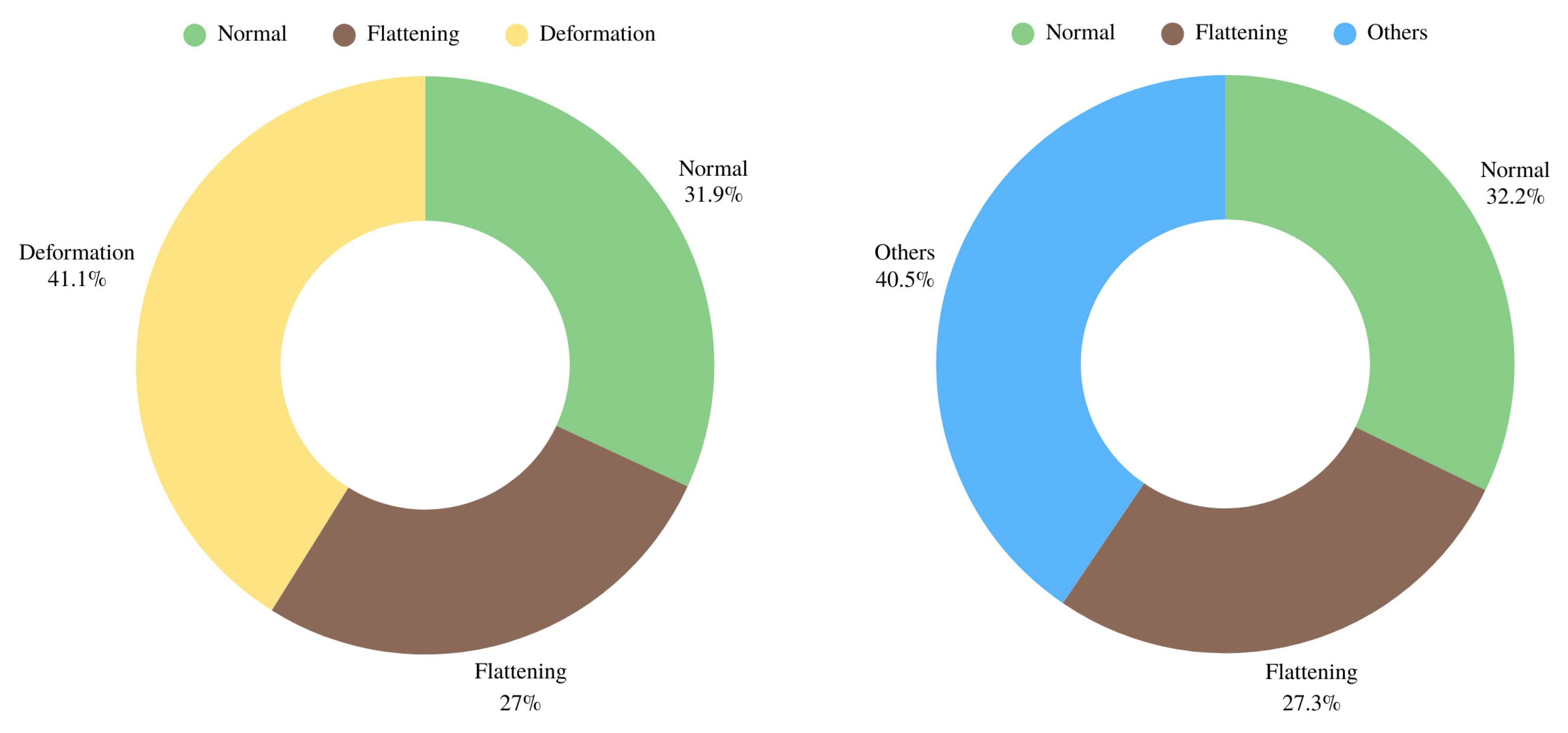
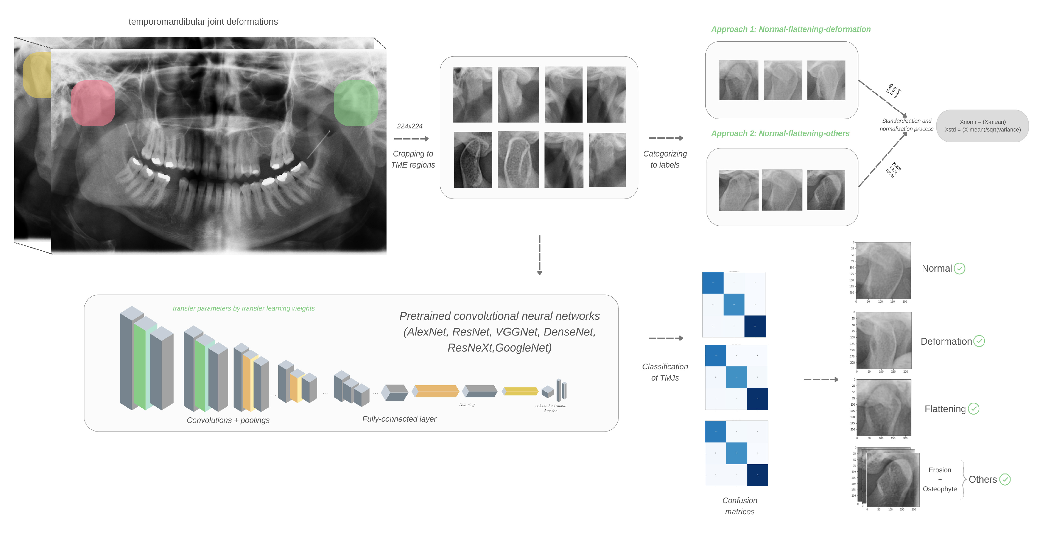
2.1. Selection, Preparation and Evaluation of Images
2.2. Dataset and Preprocessing Steps
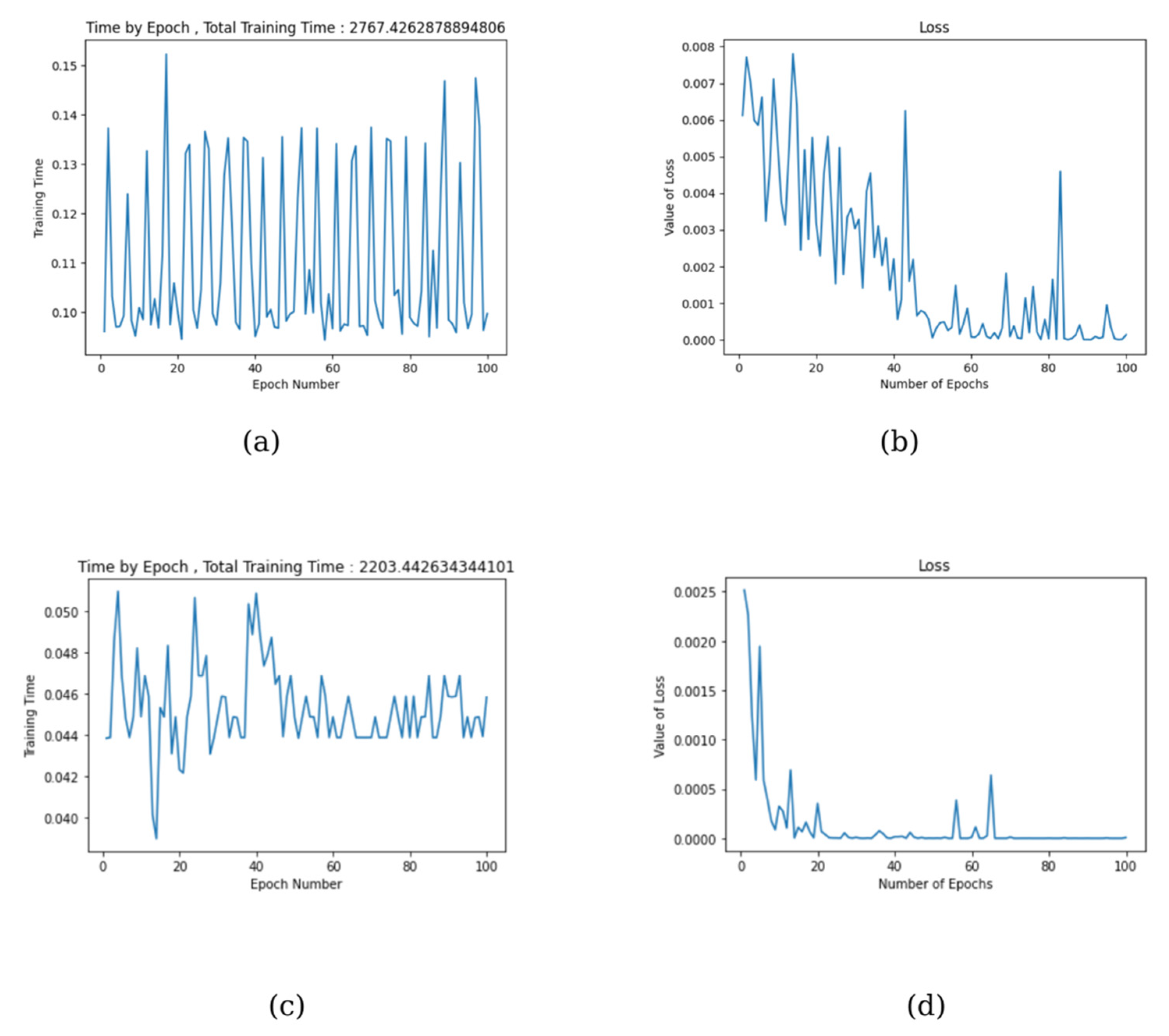
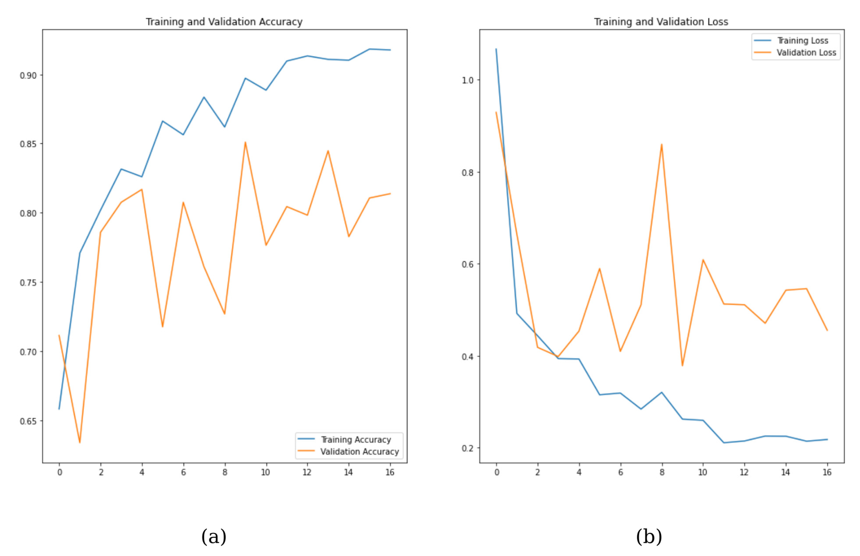
3. Results
4. Discussion
5. Conclusions
Author Contributions
Funding
Institutional Review Board Statement
Informed Consent Statement
Data Availability Statement
Conflicts of Interest
References
- Sritara, S.; Tsutsumi, M.; Fukino, K.; Matsumoto, Y.; Ono, T.; Akita, K. Evaluating the morphological features of the lateral pterygoid insertion into the medial surface of the condylar process. Clin. Exp. Dent. Res. 2021, 7, 219–225. [Google Scholar] [CrossRef] [PubMed]
- Suh, M.; Park, S.; Kim, Y.-K.; Yun, P.-Y.; Lee, W. 18F-NaF PET/CT for the evaluation of temporomandibular joint disorder. Clin. Radiol. 2018, 73, 414.e7–414.e13. [Google Scholar] [CrossRef] [PubMed]
- Minervini, G.; D’Amico, C.; Cicciù, M.; Fiorillo, L. Temporomandibular joint disk displacement: Etiology, diagnosis, imaging, and therapeutic approaches. J. Craniofacial Surg. 2023, 34, 1115–1121. [Google Scholar] [CrossRef] [PubMed]
- Crincoli, V.; Anelli, M.G.; Quercia, E.; Piancino, M.G.; Di Comite, M. Temporomandibular disorders and oral features in early rheumatoid arthritis patients: An observational study. Int. J. Med. Sci. 2019, 16, 253. [Google Scholar] [CrossRef]
- Schiffman, E.; Ohrbach, R.; Truelove, E.; Look, J.; Anderson, G.; Goulet, J.-P.; List, T.; Svensson, P.; Gonzalez, Y.; Lobbezoo, F. Diagnostic criteria for temporomandibular disorders (DC/TMD) for clinical and research applications: Recommendations of the International RDC/TMD Consortium Network and Orofacial Pain Special Interest Group. J. Oral Facial Pain Headache 2014, 28, 6. [Google Scholar] [CrossRef]
- Zieliński, G.; Pająk-Zielińska, B.; Ginszt, M. A meta-analysis of the global prevalence of temporomandibular disorders. J. Clin. Med. 2024, 13, 1365. [Google Scholar] [CrossRef]
- Bliddal, H. Definition, pathology and pathogenesis of osteoarthritis. Ugeskr. Laeger 2020, 182, V06200477. [Google Scholar]
- Cardoneanu, A.; Macovei, L.A.; Burlui, A.M.; Mihai, I.R.; Bratoiu, I.; Rezus, I.I.; Richter, P.; Tamba, B.-I.; Rezus, E. Temporomandibular joint osteoarthritis: Pathogenic mechanisms involving the cartilage and subchondral bone, and potential therapeutic strategies for joint regeneration. Int. J. Mol. Sci. 2022, 24, 171. [Google Scholar] [CrossRef]
- Mureșanu, S.; Hedeșiu, M.; Iacob, L.; Eftimie, R.; Olariu, E.; Dinu, C.; Jacobs, R.; Team Project Group. Automating Dental Condition Detection on Panoramic Radiographs: Challenges, Pitfalls, and Opportunities. Diagnostics 2024, 14, 2336. [Google Scholar] [CrossRef]
- ArunKumar, G. Bone changes in condyles of asymptomatic temperomandibular joints & its correlation with age, gender and occlusal condition; a digital panoramic study. J. Dent. Health Oral Disord. Ther. 2021, 12, 111–115. [Google Scholar]
- Görürgöz, C.; İçen, M.; Kurt, M.; Aksoy, S.; Bakırarar, B.; Rozylo-Kalinowska, I.; Orhan, K. Degenerative changes of the mandibular condyle in relation to the temporomandibular joint space, gender and age: A multicenter CBCT study. Dent. Med. Probl. 2023, 60, 127–135. [Google Scholar] [CrossRef] [PubMed]
- Schroder, Â.G.D.; Gonçalves, F.M.; Germiniani, J.d.S.; Schroder, L.D.; Porporatti, A.L.; Zeigelboim, B.S.; de Araujo, C.M.; Santos, R.S.; Stechman-Neto, J. Diagnosis of TMJ degenerative diseases by panoramic radiography: Is it possible? A systematic review and meta-analysis. Clin. Oral Investig. 2023, 27, 6395–6412. [Google Scholar] [CrossRef] [PubMed]
- Valesan, L.F.; Da-Cas, C.D.; Réus, J.C.; Denardin, A.C.S.; Garanhani, R.R.; Bonotto, D.; Januzzi, E.; de Souza, B.D.M. Prevalence of temporomandibular joint disorders: A systematic review and meta-analysis. Clin. Oral Investig. 2021, 25, 441–453. [Google Scholar] [CrossRef]
- Mani, F.M.; Sivasubramanian, S.S. A study of temporomandibular joint osteoarthritis using computed tomographic imaging. Biomed. J. 2016, 39, 201–206. [Google Scholar] [CrossRef]
- Osiewicz, M.; Kojat, P.; Gut, M.; Kazibudzka, Z.; Pytko-Polończyk, J. Self-Perceived Dentists’ Knowledge of Temporomandibular Disorders in Krakow: A Pilot Study. Pain Res. Manag. 2020, 2020, 9531806. [Google Scholar] [CrossRef]
- Mozhdeh, M.; Caroccia, F.; Moscagiuri, F.; Festa, F.; D’Attilio, M. Evaluation of knowledge among dentists on symptoms and treatments of temporomandibular disorders in Italy. Int. J. Environ. Res. Public Health 2020, 17, 8760. [Google Scholar] [CrossRef]
- Schwendicke, F.; Golla, T.; Dreher, M.; Krois, J. Convolutional neural networks for dental image diagnostics: A scoping review. J. Dent. 2019, 91, 103226. [Google Scholar] [CrossRef]
- Shafi, I.; Fatima, A.; Afzal, H.; Díez, I.D.L.T.; Lipari, V.; Breñosa, J.; Ashraf, I. A Comprehensive Review of Recent Advances in Artificial Intelligence for Dentistry E-Health. Diagnostics 2023, 13, 2196. [Google Scholar] [CrossRef]
- Özbay, Y.; Kazangirler, B.Y.; Özcan, C.; Pekince, A. Detection of the separated endodontic instrument on periapical radiographs using a deep learning-based convolutional neural network algorithm. Aust. Endod. J. 2024, 50, 131–139. [Google Scholar] [CrossRef]
- Bayrakdar, I.S.; Orhan, K.; Akarsu, S.; Çelik, Ö.; Atasoy, S.; Pekince, A.; Yasa, Y.; Bilgir, E.; Sağlam, H.; Aslan, A.F. Deep-learning approach for caries detection and segmentation on dental bitewing radiographs. Oral Radiol. 2022, 38, 468–479. [Google Scholar] [CrossRef]
- Kreiner, M.; Viloria, J. A novel artificial neural network for the diagnosis of orofacial pain and temporomandibular disorders. J. Oral Rehabil. 2022, 49, 884–889. [Google Scholar] [CrossRef] [PubMed]
- Chauhan, R.; Ghanshala, K.K.; Joshi, R. Convolutional neural network (CNN) for image detection and recognition. In Proceedings of the 2018 First International Conference on Secure Cyber Computing and Communication (ICSCCC), Jalandhar, India, 15–17 December 2018; IEEE: Piscataway, NJ, USA, 2018; pp. 278–282. [Google Scholar]
- Ozsari, S.; Güzel, M.S.; Yılmaz, D.; Kamburoğlu, K. A Comprehensive Review of Artificial Intelligence Based Algorithms Regarding Temporomandibular Joint Related Diseases. Diagnostics 2023, 13, 2700. [Google Scholar] [CrossRef] [PubMed]
- Zhu, Z.; Lin, K.; Jain, A.K.; Zhou, J. Transfer learning in deep reinforcement learning: A survey. IEEE Trans. Pattern Anal. Mach. Intell. 2023, 45, 13344–13362. [Google Scholar] [CrossRef]
- Shaha, M.; Pawar, M. Transfer learning for image classification. In Proceedings of the 2018 Second International Conference on Electronics, Communication and Aerospace Technology (ICECA), Coimbatore, India, 29–31 March 2018; IEEE: Piscataway, NJ, USA, 2018; pp. 656–660. [Google Scholar]
- Farook, T.H.; Dudley, J. Automation and deep (machine) learning in temporomandibular joint disorder radiomics: A systematic review. J. Oral Rehabil. 2023, 50, 501–521. [Google Scholar] [CrossRef]
- Yazici, İ.; Shayea, I.; Din, J. A survey of applications of artificial intelligence and machine learning in future mobile networks-enabled systems. Eng. Sci. Technol. Int. J. 2023, 44, 101455. [Google Scholar] [CrossRef]
- Nishiyama, M.; Ishibashi, K.; Ariji, Y.; Fukuda, M.; Nishiyama, W.; Umemura, M.; Katsumata, A.; Fujita, H.; Ariji, E. Performance of deep learning models constructed using panoramic radiographs from two hospitals to diagnose fractures of the mandibular condyle. Dentomaxillofacial Radiol. 2021, 50, 20200611. [Google Scholar] [CrossRef]
- Ahn, Y.; Hwang, J.J.; Jung, Y.-H.; Jeong, T.; Shin, J. Automated mesiodens classification system using deep learning on panoramic radiographs of children. Diagnostics 2021, 11, 1477. [Google Scholar] [CrossRef]
- Lee, K.; Kwak, H.; Oh, J.; Jha, N.; Kim, Y.; Kim, W.; Baik, U.; Ryu, J. Automated detection of TMJ osteoarthritis based on artificial intelligence. J. Dent. Res. 2020, 99, 1363–1367. [Google Scholar] [CrossRef]
- Choi, E.; Kim, D.; Lee, J.-Y.; Park, H.-K. Artificial intelligence in detecting temporomandibular joint osteoarthritis on orthopantomogram. Sci. Rep. 2021, 11, 10246. [Google Scholar] [CrossRef]
- Jung, W.; Lee, K.; Suh, B.; Seok, H.; Lee, D. Deep learning for osteoarthritis classification in temporomandibular joint. Oral Dis. 2023, 29, 1050–1059. [Google Scholar] [CrossRef]
- Hegde, S.; Praveen, B.; Shetty, S.R. Morphological and radiological variations of mandibular condyles in health and diseases: A systematic review. Dentistry 2013, 3, 154. [Google Scholar]
- Mallya, S.; Lam, E. White and Pharoah’s Oral Radiology: Principles and Interpretation; Elsevier Health Sciences: Chennai, India, 2018. [Google Scholar]
- Tekin, B.Y.; Ozcan, C.; Pekince, A.; Yasa, Y. An enhanced tooth segmentation and numbering according to FDI notation in bitewing radiographs. Comput. Biol. Med. 2022, 146, 105547. [Google Scholar]
- Szegedy, C.; Liu, W.; Jia, Y.; Sermanet, P.; Reed, S.; Anguelov, D.; Erhan, D.; Vanhoucke, V.; Rabinovich, A. Going deeper with convolutions. In Proceedings of the IEEE Conference on Computer Vision and Pattern Recognition, Boston, MA, USA, 1–12 June 2015; pp. 1–9. [Google Scholar]
- Pekince, K.A.; Caglayan, F.; Pekince, A. Imaging of masseter muscle spasms by ultrasonography: A preliminary study. Oral Radiol. 2020, 36, 85–88. [Google Scholar] [CrossRef] [PubMed]
- Pekince, K.A.; Çağlayan, F.; Pekince, A. The efficacy and limitations of USI for diagnosing TMJ internal derangements. Oral Radiol. 2020, 36, 32–39. [Google Scholar] [CrossRef]
- Walewski, L.Â.; de Souza Tolentino, E.; Yamashita, F.C.; Iwaki, L.C.V.; da Silva, M.C. Cone beam computed tomography study of osteoarthritic alterations in the osseous components of temporomandibular joints in asymptomatic patients according to skeletal pattern, gender, and age. Oral Surg. Oral Med. Oral Pathol. Oral Radiol. 2019, 128, 70–77. [Google Scholar] [CrossRef]
- Schmitter, M.; Gabbert, O.; Ohlmann, B.; Hassel, A.; Wolff, D.; Rammelsberg, P.; Kress, B. Assessment of the reliability and validity of panoramic imaging for assessment of mandibular condyle morphology using both MRI and clinical examination as the gold standard. Oral Surg. Oral Med. Oral Pathol. Oral Radiol. Endodontology 2006, 102, 220–224. [Google Scholar] [CrossRef]
- Singh, B.; Kumar, N.R.; Balan, A.; Nishan, M.; Haris, P.S.; Jinisha, M.; Denny, C.D. Evaluation of normal morphology of mandibular condyle: A radiographic survey. J. Clin. Imaging Sci. 2020, 10, 51. [Google Scholar] [CrossRef]
- Abrahamsson, A.-K.; Kristensen, M.; Arvidsson, L.Z.; Kvien, T.K.; Larheim, T.A.; Haugen, I.K. Frequency of temporomandibular joint osteoarthritis and related symptoms in a hand osteoarthritis cohort. Osteoarthr. Cartil. 2017, 25, 654–657. [Google Scholar] [CrossRef]
- Sonnesen, L.; Petersson, A.; Wiese, M.; Jensen, K.E.; Svanholt, P.; Bakke, M. Osseous osteoarthritic-like changes and joint mobility of the temporomandibular joints and upper cervical spine: Is there a relation? Oral Surg. Oral Med. Oral Pathol. Oral Radiol. 2017, 123, 273–279. [Google Scholar] [CrossRef]
- Dumbuya, A.; Gomes, A.F.; Marchini, L.; Zeng, E.; Comnick, C.L.; Melo, S.L.S. Bone changes in the temporomandibular joints of older adults: A cone-beam computed tomography study. Spec. Care Dent. 2020, 40, 84–89. [Google Scholar] [CrossRef]
- de Dumast, P.; Mirabel, C.; Cevidanes, L.; Ruellas, A.; Yatabe, M.; Ioshida, M.; Ribera, N.T.; Michoud, L.; Gomes, L.; Huang, C.; et al. A web-based system for neural network based classification in temporomandibular joint osteoarthritis. Comput. Med. Imaging Graph. 2018, 67, 45–54. [Google Scholar] [CrossRef]

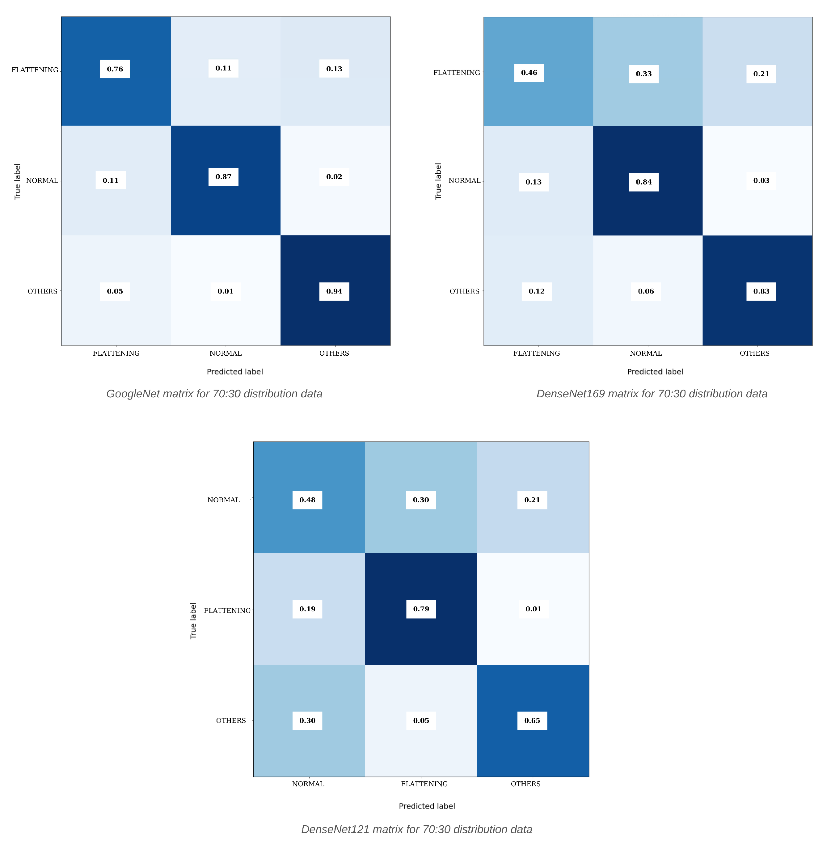
| Model | Distribution | Learning Rate | Optimizer | Accuracy | Precision | Recall | F1-Score |
|---|---|---|---|---|---|---|---|
| DenseNet121 | 70:30 | 0.001 | Adamax | 64.85% | 64.45% | 64.22% | 63.88% |
| ResNet18 | 70:30 | 0.0001 | Adamax | 69.23% | 65.52% | 66.41% | 65.65% |
| AlexNet | 70:30 | 0.0001 | Adamax | 70.71% | 68.74% | 68.55% | 68.47% |
| DenseNet169 | 70:30 | 0.0001 | Adamax | 73.43% | 71.05% | 71.04% | 70.66% |
| GoogleNet | 70:30 | 0.0001 | Adamax | 86.61% | 85.92% | 85.60% | 85.73% |
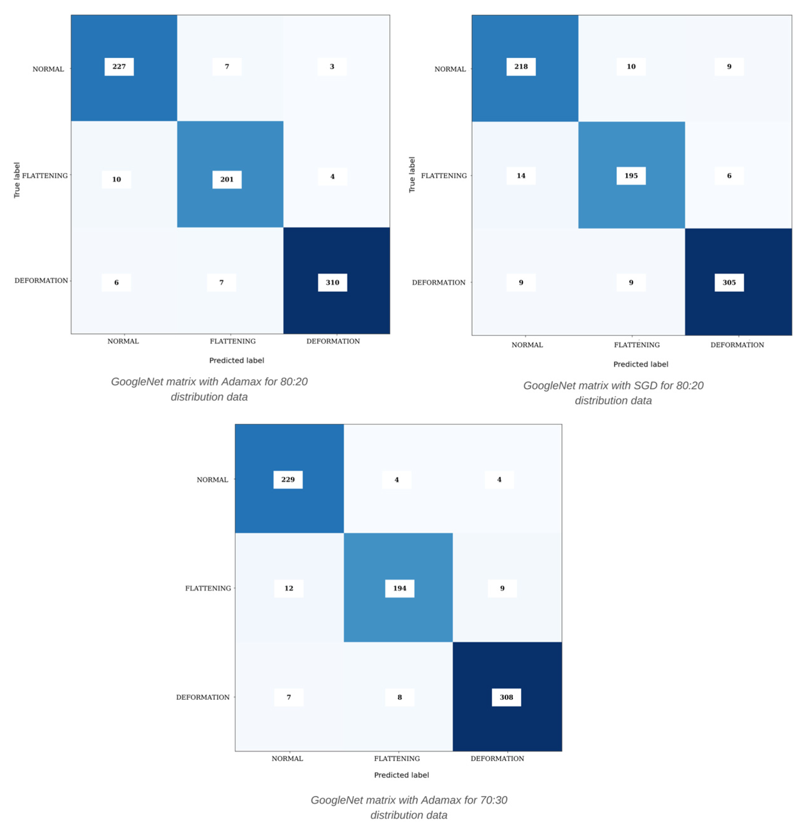
| Model | Distribution | Dataset | Optimizer | Accuracy | Precision | Recall | F1-Score |
|---|---|---|---|---|---|---|---|
| DenseNet169 | 70:30 | N-F-O | Adamax | 73.43% | 73.29% | 73.12% | 73.20% |
| GoogleNet | 70:30 | N-F-O | Adamax | 86.61% | 85.92% | 85.60% | 85.73% |
| GoogleNet | 80:20 | N-F-D | SGD | 92.65% | 92.29% | 92.36% | 92.33% |
| ResNeXt | 80:20 | N-F-D | Adamax | 94.32% | 94.15% | 94.07% | 94.08% |
| GoogleNet | 80:20 | N-F-D | Adamax | 95.23% | 94.89% | 95.08% | 94.98% |
Disclaimer/Publisher’s Note: The statements, opinions and data contained in all publications are solely those of the individual author(s) and contributor(s) and not of MDPI and/or the editor(s). MDPI and/or the editor(s) disclaim responsibility for any injury to people or property resulting from any ideas, methods, instructions or products referred to in the content. |
© 2025 by the authors. Licensee MDPI, Basel, Switzerland. This article is an open access article distributed under the terms and conditions of the Creative Commons Attribution (CC BY) license (https://creativecommons.org/licenses/by/4.0/).
Share and Cite
Azlağ Pekince, K.; Pekince, A.; Kazangirler, B.Y. Improving TMJ Diagnosis: A Deep Learning Approach for Detecting Mandibular Condyle Bone Changes. Diagnostics 2025, 15, 1022. https://doi.org/10.3390/diagnostics15081022
Azlağ Pekince K, Pekince A, Kazangirler BY. Improving TMJ Diagnosis: A Deep Learning Approach for Detecting Mandibular Condyle Bone Changes. Diagnostics. 2025; 15(8):1022. https://doi.org/10.3390/diagnostics15081022
Chicago/Turabian StyleAzlağ Pekince, Kader, Adem Pekince, and Buse Yaren Kazangirler. 2025. "Improving TMJ Diagnosis: A Deep Learning Approach for Detecting Mandibular Condyle Bone Changes" Diagnostics 15, no. 8: 1022. https://doi.org/10.3390/diagnostics15081022
APA StyleAzlağ Pekince, K., Pekince, A., & Kazangirler, B. Y. (2025). Improving TMJ Diagnosis: A Deep Learning Approach for Detecting Mandibular Condyle Bone Changes. Diagnostics, 15(8), 1022. https://doi.org/10.3390/diagnostics15081022