Abstract
The air kerma, which is the amount of energy given off by a radioactive substance, is essential for medical specialists who use radiation to diagnose cancer problems. The amount of energy that a photon has when it hits something can be described as the air kerma (the amount of energy that was deposited in the air when the photon passed through it). Radiation beam intensity is represented by this value. Hospital X-ray equipment has to account for the heel effect, which means that the borders of the picture obtain a lesser radiation dosage than the center, and that air kerma is not symmetrical. The voltage of the X-ray machine can also affect the uniformity of the radiation. This work presents a model-based approach to predict air kerma at various locations inside the radiation field of medical imaging instruments, making use of just a small number of measurements. Group Method of Data Handling (GMDH) neural networks are suggested for this purpose. Firstly, a medical X-ray tube was modeled using Monte Carlo N Particle (MCNP) code simulation algorithm. X-ray tubes and detectors make up medical X-ray CT imaging systems. An X-ray tube’s electron filament, thin wire, and metal target produce a picture of the electrons’ target. A small rectangular electron source modeled electron filaments. An electron source target was a thin, 19,290 kg/m3 tungsten cube in a tubular hoover chamber. The electron source–object axis of the simulation object is 20° from the vertical. For most medical X-ray imaging applications, the kerma of the air was calculated at a variety of discrete locations within the conical X-ray beam, providing an accurate data set for network training. Various locations were taken into account in the aforementioned voltages inside the radiation field as the input of the GMDH network. For diagnostic radiology applications, the trained GMDH model could determine the air kerma at any location in the X-ray field of view and for a wide range of X-ray tube voltages with a Mean Relative Error (MRE) of less than 0.25%. This study yielded the following results: (1) The heel effect is included when calculating air kerma. (2) Computing the air kerma using an artificial neural network trained with minimal data. (3) An artificial neural network quickly and reliably calculated air kerma. (4) Figuring out the air kerma for the operating voltage of medical tubes. The high accuracy of the trained neural network in determining air kerma guarantees the usability of the presented method in operational conditions.
1. Introduction
There are two steps in the process by which photons impart their energy to matter. The interaction of photons with matter first transfers energy to the charge carriers of matter. The charge carriers’ kinetic energy is then deposited by the ionized and excited atoms. By dividing the total kinetic energy of the charged particles (such as electrons, protons, and other charged atoms) that are released when the rays impact something, we may obtain a measure of the radiation that goes through that item; this measure is called the kerma. Kinetic energy divided by matter mass yields this value [1]. Ionizing radiation without a charge is referred to as “kerma” by scientists. The quantity of radiation that has been absorbed is equal to the amount of kerma, which is measured in gray. A mass of air has the same amount of kerma as another mass of air. As measuring air kerma is much easier than measuring the dosage, it is often used for radiation equipment calibration [2]. In interventional radiology, if the skin dosage is high enough to induce radiographic burns to the patient, air kerma computation is also used to forecast the skin dose [3]. Researchers have recently been interested in studying the air kerma created by X-ray tubes. Another article looked at how changing the anode angle or the wave voltage of the X-ray tube affected the air kerma. A Philips MCN165 was used to test the X-ray tube model at a voltage range of 40 to 140 kV [4]. In this investigation, it was found that raising the anode angle had the same effect on airflow as raising the supply voltage. They also claim that the air kerma lessens the severity of wrinkles. After introducing the Monte Carlo simulator for a sodium iodide detector, Oliveira et al. [5] developed a spectral separation method for determining the air kerma from X-rays. Without the suggested spectrum stripping procedure, the discrepancy between the derived spectrum and the reference spectrum was over 63%, but it was reduced to less than 0.2%. The kerma of the chest wall in kids and teens was investigated by Porto et al. [6]. According to the findings of this study, air tension falls as tube voltage rises and exposure falls. Air kerma has been measured and reported on by researchers in the medical and industrial sectors [7,8,9,10,11,12,13,14,15]. These analyses did not include the rest of the X-ray tube’s radiation field in their estimation of air kerma at the tube’s core. It should be noted that the quantity of air kerma changes with the angle inside the X-ray beam, even when the anode is kept at a constant distance. The anode heel effect is the source of this discrepancy. These analyses did not include the rest of the X-ray tube’s radiation field in their estimation of air kerma at the tube’s core. Notably, the quantity of air kerma changes with distance from the anode in the radiation field. The anode heel effect is to blame for the discrepancy between these values. Some researchers have investigated the heel effect in the radiation field. In Ref. [16] researchers have tried to determine air kerma using an intelligent method. Although they used the MLP neural network to predict air kerma, the accuracy of the methodology they presented in air kerma prediction was not high. In the next research [17], the researchers investigated the performance of the RBF neural network for forecasting air kerma. Although the accuracy increased, it is predicted that by selecting the appropriate neural network, the accuracy in determining air kerma can be increased even more. Despite the existence of the anode heel effect, this research presents a technique for accurately estimating air kerma. The air kerma was computed and simulated using the Monte Carlo N Particle (MCNP) algorithm at six different X-ray tube voltages and various distances to the source. Using the MCNP code’s sparse data, a Group Method of Data Handling (GMDH) neural network is trained to generate predictions about the air kerma. The trained neural network can calculate the air kerma for any given X-ray tube voltage and position in the X-ray field. While the MCNP algorithm may be used to calculate air kerma, this is a time-consuming procedure, hence it is more efficient to employ a neural network to make predictions about air kerma. The present investigation is organized as follows: A thorough description of the structure that the MCNP algorithm simulates is provided in Section 2. In the next section, these simulation data are used to teach the GMDH neural network. The findings and conclusions are presented in Section 4 and Section 5, respectively.
The following are some of the major findings of this study.
- The heel effect is taken into account while calculating air kerma.
- Calculating the air kerma by employing an artificial neural network and training it with a limited amount of data in varying angles, distances, and voltages of tubes.
- Using an artificial neural network, the calculation of air kerma was executed extremely quickly and accurately compared to earlier efforts.
- Calculating the air kerma for medical tubes’ operating voltage.
2. Methodology
As shown in Figure 1, the two main components of a medical X-ray CT imaging system are the X-ray tube and the detector. An X-ray tube’s electron filament (a thin wire) and metal target allow for the production of an X-ray image (the object the electrons hit). After being generated by the filament, electrons are propelled through a large potential difference in the X-ray source’s hoover chamber before striking the target. The Bremsstrahlung process converts just a small proportion of the energy in electrons into photons, therefore most of the energy ends up as heat. Several projections, or 2D pictures, are taken when the X-ray tube and detector spin around the subject at the same time. The system takes 2D photos of the patient and uses powerful computer technology to recreate 3D images of their body in accordance with Lambert Beer’s law. In the medical X-ray imaging sector, air kerma has only been studied using a model of an X-ray tube (as shown in Figure 2). A medical X-ray tube is simulated using code written in MCNPX. To model electron filaments, a tiny rectangular electron source was examined. If you want to simulate focal spots, you will need to use a surface source rather than a point source. A thin tungsten cube with a density of 19,290 kg/m3 was placed in a tubular vacuum chamber as an electron source target. The electron source–object axis of the simulation object has an angle of 20° to the vertical. It is important to note that at the maximum tilt angle of the X-ray tube target, the emitted X-rays leave the tube within the cone. To create the illusion of a hoover chamber, the electrons and the target are encased in a steel shell. The only section of the hoover chamber that has any action was the exposed circle. At the entrance to the vacuum chamber is a beryllium window with a density of 1850 kg/m3 and a thickness of 1 mm. Two-stage point detector counting was used to determine air kerma (tally F5). At each detector, the photon flux was first measured. The floating air kerma conversion factor recommended in the ICRP-51 report of the International Committee on Radiation Protection was used to determine the air kerma in the second stride [18]. It should be noted that the overall statistical uncertainty did not exceed 4% in all Monte Carlo simulations in this study. In this article, we employ a spherical coordinate system to precisely locate point detectors (according to the inherent spherical symmetry of the X-rays produced) at various tangent angles (0°, 2°, 4°, 6°, 8°, and 10°, point detectors were placed at 25, 50, 75, 100, and 125 mm from the source at 12°, 14°, 16°, 18°, and 20°, respectively) and polar angles (Φ = 0°, 15°, 30°, 45°, 60°, 75°, 90°, 105°, 120°, 135°, 150°, 165°, 180°, 195°, 210°, 225°, 240°, 255°, 270°, 285°, 350°, 330°, 345°, and 360°). The air kerma was calculated from the installed control points for tube voltages of 40, 60, 80, 100, 120, and 140 kV. Calculating the air kerma map for a given set of parameters required about 96 h when using a personal computer with an Intel(R) Core(TM) i7 CPU and 8GB RAM for Monte Carlo simulation.
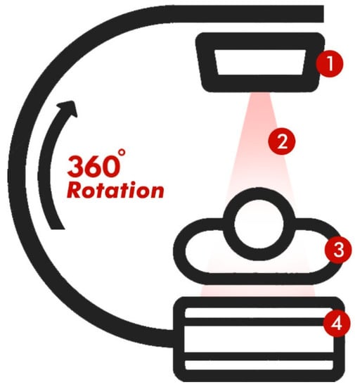
Figure 1.
A medical X-ray computed tomography imaging system: (1) X-ray tube, (2) conical X-ray beam, (3) patient, and (4) detector.
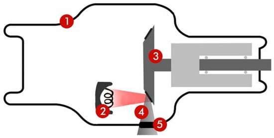
Figure 2.
The X-ray tube: (1) shield, (2) electron filament, (3) target, (4) X-ray radiation beam, and (5) window.
GMDH Neural Network
In recent years, researchers have used mathematical models called artificial neural networks to help them understand how radiation interacts with tissue [18,19,20,21,22,23,24,25,26,27,28,29,30,31]. Moreover, the strong mathematical tool of numerical computing [32,33,34,35,36,37,38] has been employed to solve various engineering challenges, most notably in the field of artificial networks [39,40,41,42,43,44]. One of the intelligent methods for solving complex and nonlinear problems was developed in 1968 by M.G. Ivakhnenko and named GMDH [45]. In fact, these algorithms create self-examination methods with prediction, classification, control synthesis, and system debugging capabilities. The characteristics of the network structure, including the number of layers, the number of important input features, and the ideal network configuration, were all detected automatically using Ivahnenko’s method. This method presumes that Kolmogorov–Gabor polynomials of higher order determine the system’s input and output equations.
x(x1, x2, …, xm) represents the input (the features vector), a(a1, a2, …, am) represents the coefficient or weight, and y(x) represents the network’s output. The following procedures should have been carried out in order to use a GMDH network:
In the first step, new variables should have been created and quadratic regression polynomials are calculated based on Equation (2) for each combination and two at a time for all characteristics (x1, x2…xm).
Coefficient C was determined using the least squares method in this investigation. Take note of how each of the quadratic polynomials computed is quite close to the target value. A quadratic polynomial is calculated by each neuron. Secondly, dead neurons are those that could not accurately forecast the required product. The leftover neurons are employed for the layer-up procedure. This process not only creates the first neural layer, but also chooses the most effective neurons. The third phase involves using the polynomial found in the second stage to generate the next layer. This means that the old polynomial is used as a basis for creating a new polynomial, and the second step is repeated until an effective neuron is located. The GMDH neural network is not complete until this process is repeated several times. In the final stage, accuracy is guaranteed and test data are used to assess the efficiency of the designed network. Training data and test data are created throughout the neural network construction phases. The training data are used to create the neural network, and the error is minimized by tuning the network’s various parameters. After the training process is complete, the network’s effectiveness ought to be evaluated against data it has never seen before to ensure it has retained what it has learned. If this step is completed successfully, the network will behave as expected under operating circumstances. Around 70% of the data were used for training and the remaining 30% of the data were used for evaluation.
3. Results
For this research, the air kerma was calculated using a GMDH neural network. After extracting the function, it was fed into the network. For accurate air kerma estimation, the functions ϕ, θ, r, and V were found to be most useful. Figure 3 depicts the intended structure of the GMDH neural network.
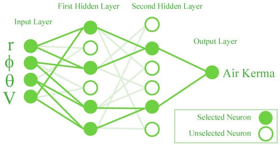
Figure 3.
The architecture of the proposed GMDH neural network.
The GMDH network took into consideration the voltage of the X-ray tube and the position inside the radiation field as inputs. Output was measured in kerma of air. A neural network was trained by randomly picking 5775 samples from the provided data. When training was complete, the remaining data was utilized to evaluate the neural network. Two hidden layers, each with 4 neurons, were able to give accurate correlations between inputs and outputs. Two error measures, mean relative error (MRE) and root mean square error (RMSE), were used to determine the discrepancy between the MCNP code’s air kerma volume and the neural network’s air kerma prediction. These requirements are represented by the following equations:
X(Exp) and X(Pred) are the experimental and predicted values, whereas N is the total number of samples.
4. Discussion
The air kerma, calculated using the Monte Carlo model, is shown in Figure 4 for two different tube voltages (60 kV and 120 kV) based on the X-ray field of view at a distance of 75 mm from the source. Figure 4a,b demonstrate how the heel effect of the X-ray tube causes the anticipated air kerma to be smaller on the right side of the field of view (towards the target) than on the left, despite being almost uniform from top to bottom. The kerma of the air increases as the voltage in the tube increases. To demonstrate the effect of distance, the air kerma is computed with the voltage held constant at 80 kV and the detector placed at distances of 500 mm and 1000 mm, respectively, in Figure 5a,b. Air kerma drops down dramatically with distance from the source, as predicted. This implies if the radiation source travels away from the treated region, the quantity of radiation that reaches that area goes lower.
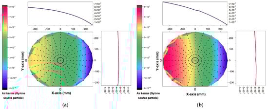
Figure 4.
The air kerma determined with the help of the Monte Carlo method at (a) 60 kV and (b) 120 kV.
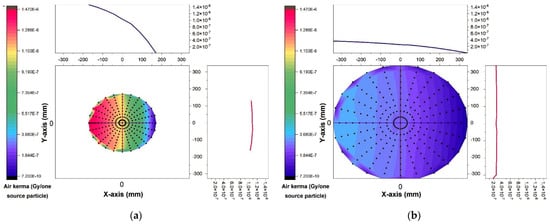
Figure 5.
The air kerma determined with the help of the Monte Carlo method at (a) 500 mm and (b) 1000 mm.
Figure 6 exhibits two error histograms and regression plots on the training and testing data to visually emphasize the neural network’s performance. In the regression graph, the green circle represents the neural network’s prediction and the yellow line represents the optimal answer (the value of air kerma generated using the MCNP algorithm). These coincide, proving the network’s high precision. Some input and output data of the GMDH neural network are displayed in Table 1. In this table, some of the tube voltage values and the location that is considered inputs of the network can be seen, along with the amount of air kerma calculated by the MCNP code. In this table, you can see the performance of the neural network in finding the input–output relationship. It should be noted that for the best possible performance of the neural network, first the inputs and outputs are normalized, and then after predicting the output, the data are returned to their initial state. The amount of air kerma predicted by the neural network is also provided. As it is clear, the value predicted by the neural network has a slight difference from the calculated value, which indicates the acceptable performance of the neural network.
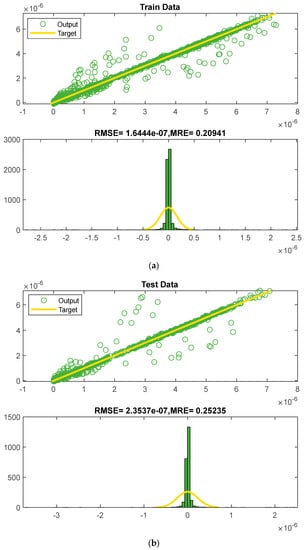
Figure 6.
Diagram of the regression and error histograms for the: (a) training and (b) test datasets.

Table 1.
Some input and output data of the GMDH neural network.
5. Conclusions
Calculating air kerma using the MCNP code is very time-consuming and applies a high volume of calculations to the system, which requires relatively powerful processors to simulate the radiation field and calculate air kerma. For this purpose, in this research, an attempt has been made to provide a quick and low calculation method for predicting this parameter by calculating air kerma at limited points. The MCNP algorithm and a neural network were used in this research to find the air kerma in the radiation field of the X-ray tube. This was accomplished by inspecting the X-ray tube at a voltage range of 40 to 140 kV. Data from 1375 points throughout the radiation field of the X-ray tube were analyzed to determine the air kerma at each voltage. The generated data matrix contains the 8250 columns (various samples) and four rows (three location attributes and X-ray voltage) needed to construct the neural network. Given the location and voltage of the X-ray tube, the supervised, fast-learning GMDH network was trained to forecast air kerma. The suggested model exhibited an MRE of less than 0.25% for predicting air kerma. Due to its excellent precision and speed, it is the most accurate approach for determining the air kerma in the radiation field of an X-ray tube. While the approach employed in this work was specifically focused on estimating air kerma for a particular X-ray tube design (fixed target angle of 20°), it may be utilized for a broad range of X-ray tube radiation fields. The suggested approach may also be used to calculate other radiation characteristics, such as absorbed dose.
Author Contributions
Methodology, L.Z., F.X., L.W., Y.C. and G.Z.; Investigation, E.N. and X.Z.; Writing—original draft, G.Z.; Supervision, L.Z. All authors have read and agreed to the published version of the manuscript.
Funding
This work is supported by the Research Foundation of Hangzhou Dianzi University (KYS335622091; KYH333122029M).
Institutional Review Board Statement
Not applicable.
Informed Consent Statement
Not applicable.
Data Availability Statement
The data presented in this study are available on request from the corresponding author.
Conflicts of Interest
The authors declare no conflict of interest.
References
- Cember, H.; Johnson, T.E. Introduction to Health Physics; McGraw-Hill Inc.: New York, NY, USA, 2009. [Google Scholar]
- Calibration of Radiation Protection. Monitoring Instruments; IAEA Safety Report No. 16; IAEA: Vienna, Austria, 2000. [Google Scholar]
- Miller, D.L.; Balter, S.; Schueler, B.A.; Wagner, L.K.; Strauss, K.J.; Vano, E. Clinical Radiation Management for Fluoroscopically Guided Interventional Procedures. Radiology 2010, 257, 321–332. [Google Scholar] [CrossRef] [PubMed]
- Katoh, Y.; Mita, S.; Fukushi, M.; Nyui, Y.; Abe, S.; Kimura, J. Calculation of air-kerma rate of diagnostic X-ray generators. Radiol. Phys. Technol. 2011, 4, 1–6. [Google Scholar] [CrossRef] [PubMed]
- Oliveira, L.S.R.; Conti, C.C.; Amorim, A.S.; Balthar, M.C.V. NaI (Tl) scintillator detectors stripping procedure for air kerma measurements of diagnostic X-ray beams. Nucl. Instrum. Methods Phys. Res. 2013, 705, 106–110. [Google Scholar] [CrossRef]
- Porto, L.; Lunelli, N.; Paschuk, S.; Oliveira, A.; Ferreira, J.; Schelin, H.; Miguel, C.; Denyak, V.; Kmiecik, C.; Tilly, J.; et al. Evaluation of entrance surface air kerma in pediatric chest radiography. Radiat. Phys. Chem. 2014, 104, 252–259. [Google Scholar] [CrossRef]
- Alonso, T.C.; Mourão Filho, A.P.; Da Silva, T.A. Measurements of air kerma index in computed tomography: A comparison among methodologies. Appl. Radiat. Isot. 2018, 138, 10–13. [Google Scholar] [CrossRef]
- Haba, T.; Koyama, S.; Aoyama, T.; Kinomura, Y.; Ida, Y.; Kobayashi, M.; Kameyama, H.; Tsutsumi, Y. Pin-photodiode array for the measurement of fan-beam energy and air kerma distributions of X-ray CT scanners. Phys. Medica 2016, 32, 905–913. [Google Scholar] [CrossRef]
- Kwon, D.; Little, M.P.; Miller, D.L. Reference air kerma and kerma-area product as estimators of peak skin dose for fluoroscopically guided interventions. Med. Phys. 2011, 38, 4196–4204. [Google Scholar] [CrossRef]
- Bushberg, J.T.; Seibert, J.A.; Leidholdt, E.M., Jr.; Boone, J.M. The Essential Physics of Medical Imaging, 3rd ed.; Lippincott Williams & Wilkins: Philadelphia, PA, USA, 2012. [Google Scholar]
- Perera, H.; Williamson, J.F.; Li, Z.; Mishra, V.; Meigooni, A.S. Dosimetric Characteristics, Air-Kerma Strength Calibration and Verification of Monte Carlo Simulation for a New Ytterbium-169 Brachytherapy Source. Int. J. Radiat. Oncol. Biol. Phys. 1994, 28, 953–970. [Google Scholar] [CrossRef]
- Oliveira, C.; Salgado, J.; de Carvalho, A.F. Dose rate determinations in the Portuguese Gamma Irradiation Facility: Monte Carlo simulations and measurements. Radiat. Phys. Chem. 2000, 58, 279–285. [Google Scholar] [CrossRef]
- Liu, Y.; Wei, B.; Zhuoa, R.; Wena, D.; Ding, D.; Xu, Y.; Mao, B. Determination of the Conventional True Value of Gamma-Ray Air Kerma in a Mini-type Reference Radiation. Appl. Radiat. Isot. 2016, 118, 238–245. [Google Scholar] [CrossRef]
- Ounoughi, N.; Mavon, C.; Belafrites, A.; Fromm, M. Spatial distribution of air kerma rate and impact of accelerating voltage on the quality of an ultra soft X-ray beam generated by a cold cathode tube in air. Radiat. Meas. 2015, 80, 23–28. [Google Scholar] [CrossRef]
- Mettivier, G.; Sarno, A.; Lai, Y.; Golosio, B.; Fanti, V.; Italiano, M.E.; Jia, X.; Russo, P. Virtual Clinical Trials in 2D and 3D X-ray Breast Imaging and Dosimetry: Comparison of CPU-Based and GPU-Based Monte Carlo Codes. Cancers 2022, 14, 1027. [Google Scholar] [CrossRef]
- Nazemi, E.; Rokrok, B.; Movafeghi, A.; Dinca, M.; Kabir, M. Calculation of air kerma inside the radiation field of X-ray tube. Radiat. Meas. 2019, 124, 79–84. [Google Scholar] [CrossRef]
- Lu, Y.; Zheng, N.; Ye, M.; Zhu, Y.; Zhang, G.; Nazemi, E.; He, J. Proposing Intelligent Approach to Predicting Air Kerma within Radiation Beams of Medical X-ray Imaging Systems. Diagnostics 2023, 13, 190. [Google Scholar] [CrossRef]
- International Commission on Radiological Protection. Data for Use in Protection against External Radiation; ICRP Publication 51; Pergamon Press: Oxford, UK, 1987. [Google Scholar]
- Nazemi, E.; Movafeghi, A.; Rokrok, B.; Dastjerdi, M.H.C. A novel method for predicting pixel value distribution non-uniformity due to heel effect of X-ray tube in industrial digital radiography using artificial neural network. J. Nondestruct. Eval. 2018, 38, 3. [Google Scholar] [CrossRef]
- Sattari, M.A.; Roshani, G.H.; Hanus, R.; Nazemi, E. Applicability of time-domain feature extraction methods and artificial intelligence in two-phase flow meters based on gamma-ray absorption technique. Measurement 2021, 168, 108474. [Google Scholar] [CrossRef]
- Sattari, M.A.; Roshani, G.H.; Hanus, R. Improving the structure of two-phase flow meter using feature extraction and GMDH neural network. Radiat. Phys. Chem. 2020, 171, 108725. [Google Scholar] [CrossRef]
- Nazemi, E.; Feghhi, S.A.H.; Roshani, G.H. Void fraction prediction in two-phase flows independent of the liquid phase density changes. Radiat. Meas. 2014, 68, 49–54. [Google Scholar] [CrossRef]
- Roshani, G.H.; Hanus, R.; Khazaei, A.; Zych, M.; Nazemi, E.; Mosorov, V. Density and velocity determination for single-phase flow based on radiotracer technique and neural networks. Flow Meas. Instrum. 2018, 61, 9–14. [Google Scholar] [CrossRef]
- Roshani, G.H.; Nazemi, E.; Feghhi, S.A.H.; Setayeshi, S. Flow regime identification and void fraction prediction in two-phase flows based on gamma ray attenuation. Measurement 2015, 62, 25–32. [Google Scholar] [CrossRef]
- Roshani, G.H.; Karami, A.; Nazemi, E. An intelligent integrated approach of Jaya optimization algorithm and neuro-fuzzy network to model the stratified three-phase flow of gas–oil–water. Comput. Appl. Math. 2019, 38, 5. [Google Scholar] [CrossRef]
- Roshani, M.; Sattari, M.A.; Ali, P.J.M.; Roshani, G.H.; Nazemi, B.; Corniani, E.; Nazemi, E. Application of GMDH neural network technique to improve measuring precision of a simplified photon attenuation based two-phase flowmeter. Flow Meas. Instrum. 2020, 75, 101804. [Google Scholar] [CrossRef]
- Nazemi, E.; Roshani, G.H.; Feghhi, S.A.H.; Setayeshi, S.; Zadeh, E.E.; Fatehi, A. Optimization of a method for identifying the flow regime and measuring void fraction in a broad beam gamma-ray attenuation technique. Int. J. Hydrogen Energy 2016, 41, 7438–7444. [Google Scholar] [CrossRef]
- Roshani, G.H.; Feghhi, S.A.H.; Mahmoudi-Aznaveh, A.; Nazemi, E.; Adineh-Vand, A. Precise volume fraction prediction in oil–water–gas multiphase flows by means of gamma-ray attenuation and artificial neural networks using one detector. Measurement 2014, 51, 34–41. [Google Scholar] [CrossRef]
- Nazemi, E.; Feghhi, S.A.H.; Roshani, G.H.; Peyvandi, R.G.; Setayeshi, S. Precise Void Fraction Measurement in Two-Phase Flows Independent of the Flow Regime using gamma-ray attenuation. Nucl. Eng. Technol. 2016, 48, 64–71. [Google Scholar] [CrossRef]
- Balubaid, M.; Sattari, M.A.; Taylan, O.; Bakhsh, A.A.; Nazemi, E. Applications of discrete wavelet transform for feature extraction to increase the accuracy of monitoring systems of liquid petroleum products. Mathematics 2021, 9, 3215. [Google Scholar] [CrossRef]
- Hartman, E.J.; Keeler, J.D.; Kowalski, J.M. Layered neural networks with Gaussian hidden units as universal approxima-tors. Neural Comput. 1990, 2, 210–215. [Google Scholar] [CrossRef]
- Lalbakhsh, A.; Mohamadpour, G.; Roshani, S.; Ami, M.; Roshani, S.; Sayem, A.S.M.; Alibakhshikenari, M.; Koziel, S. Design of a compact planar transmission line for miniaturized rat-race coupler with harmonics suppression. IEEE Access 2021, 9, 129207–129217. [Google Scholar] [CrossRef]
- Hookari, M.; Roshani, S.; Roshani, S. High-efficiency balanced power amplifier using miniaturized harmonics suppressed coupler. Int. J. RF Microw. Comput.-Aided Eng. 2020, 30, e22252. [Google Scholar] [CrossRef]
- Lotfi, S.; Roshani, S.; Roshani, S.; Gilan, M.S. Wilkinson power divider with band-pass filtering response and harmonics suppression using open and short stubs. Frequenz 2020, 74, 169–176. [Google Scholar] [CrossRef]
- Jamshidi, M.; Siahkamari, H.; Roshani, S.; Roshani, S. A compact Gysel power divider design using U-shaped and T-shaped resonators with harmonics suppression. Electromagnetics 2019, 39, 491–504. [Google Scholar] [CrossRef]
- Khan, A.A.; Shaikh, Z.A.; Baitenova, L.; Mutaliyeva, L.; Moiseev, N.; Mikhaylov, A.; Laghari, A.A.; Idris, S.A.; Alshazly, H. QoS-ledger: Smart contracts and metaheuristic for secure quality-of-service and cost-efficient scheduling of medical-data processing. Electronics 2021, 10, 3083. [Google Scholar] [CrossRef]
- Yumashev, A.; Mikhaylov, A. Development of polymer film coatings with high adhesion to steel alloys and high wear resistance. Polym. Compos. 2020, 41, 2875–2880. [Google Scholar] [CrossRef]
- Alwaely, S.A.; Yousif, N.B.A.; Mikhaylov, A. Emotional development in preschoolers and socialization. Early Child Dev. Care 2020, 191, 2484–2493. [Google Scholar] [CrossRef]
- Roshani, S.; Jamshidi, M.B.; Mohebi, F.; Roshani, S. Design and modeling of a compact power divider with squared resonators using artificial intelligence. Wirel. Pers. Commun. 2021, 117, 2085–2096. [Google Scholar] [CrossRef]
- Roshani, S.; Azizian, J.; Roshani, S.; Jamshidi, M.B.; Parandin, F. Design of a miniaturized branch line microstrip coupler with a simple structure using artificial neural network. Frequenz 2022, 76, 255–263. [Google Scholar] [CrossRef]
- Khaleghi, M.; Salimi, J.; Farhangi, V.; Moradi, M.J.; Karakouzian, M. Application of Artificial Neural Network to Predict Load Bearing Capacity and Stiffness of Perforated Masonry Walls. CivilEng 2021, 2, 48–67. [Google Scholar] [CrossRef]
- Dabiri, H.; Farhangi, V.; Moradi, M.J.; Zadehmohamad, M.; Karakouzian, M. Applications of Decision Tree and Random Forest as Tree-Based Machine Learning Techniques for Analyzing the Ultimate Strain of Spliced and Non-Spliced Reinforcement Bars. Appl. Sci. 2022, 12, 4851. [Google Scholar] [CrossRef]
- Hernandez, A.M.; Boone, J.M. Tungsten anode spectral model using interpolating cubic splines: Unfiltered X-ray spectra from 20 kV to 640 kV. Med. Phys. 2014, 41, 042101. [Google Scholar] [CrossRef]
- Zhang, G.; Liu, R.; Ge, Y.; Mayet, A.M.; Chan, S.; Li, G.; Nazemi, E. Investigation on the Wilson Neuronal Model: Optimized Approximation and Digital Multiplierless Implementation. IEEE Trans. Biomed. Circuits Syst. 2022, 16, 1181–1190. [Google Scholar] [CrossRef]
- Ivakhnenko, A.G. Polynomial Theory of Complex Systems. IEEE Trans. Syst. Man Cybern. 1971, SMC-1, 364e378. [Google Scholar] [CrossRef]


Disclaimer/Publisher’s Note: The statements, opinions and data contained in all publications are solely those of the individual author(s) and contributor(s) and not of MDPI and/or the editor(s). MDPI and/or the editor(s) disclaim responsibility for any injury to people or property resulting from any ideas, methods, instructions or products referred to in the content. |
© 2023 by the authors. Licensee MDPI, Basel, Switzerland. This article is an open access article distributed under the terms and conditions of the Creative Commons Attribution (CC BY) license (https://creativecommons.org/licenses/by/4.0/).