
Alzheimer Disease Classification through Transfer Learning Approach


Abstract
1. Introduction
- A customized convolutional neural network with transfer learning is proposed for the classification of Alzheimer’s disease.
- A new corpus, consisting of four different types of AD, is developed. Each type consists of 1254 images.
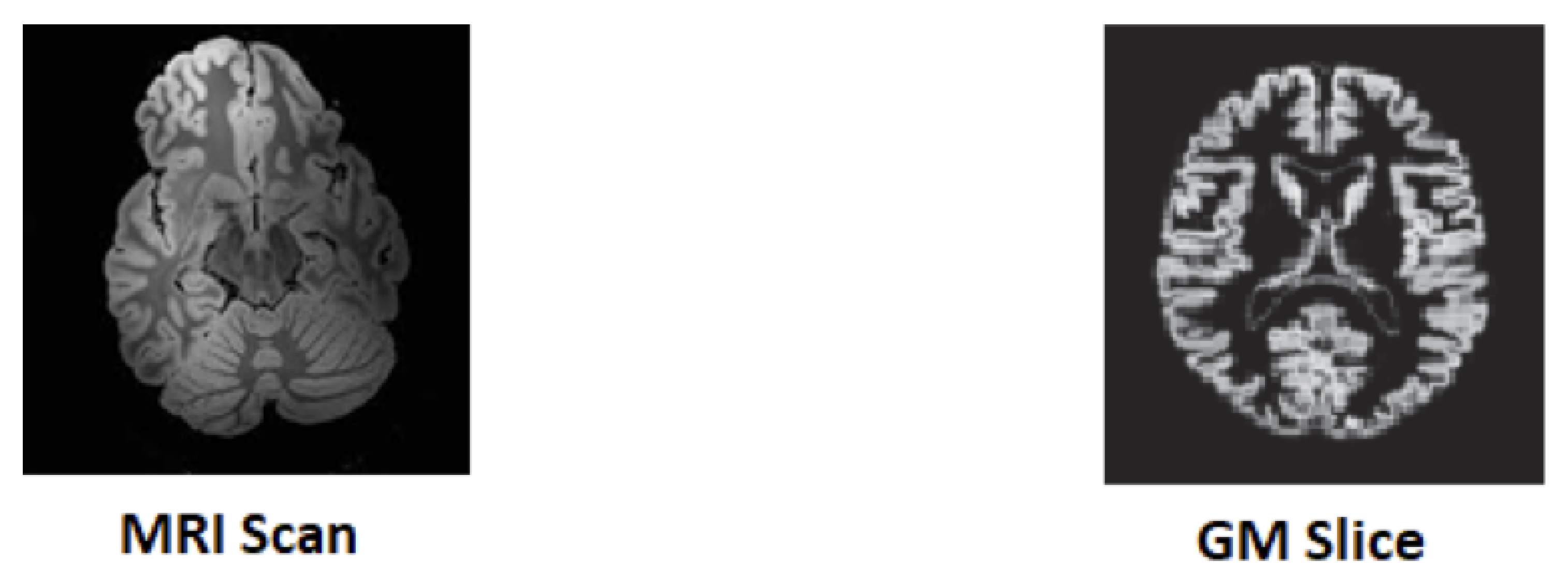
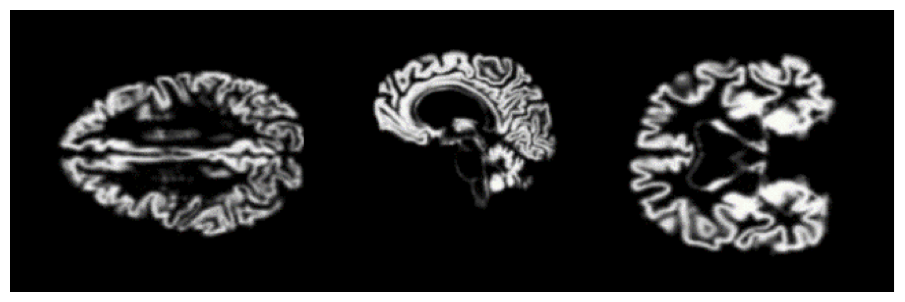
- Extraction of 2D GM slices, using “SPM12”, which is very familiar in medical image pre-processing.
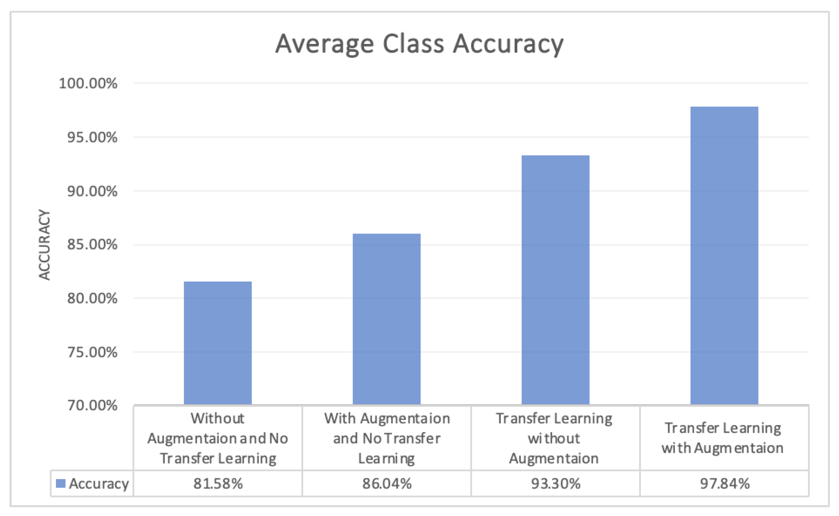
- Higher accuracy 97.84%, with a lower number of epochs, is achieved for the multi-class classification of AD.
2. Background
2.1. Convolutional Neural Network
- Convolution
- Pooling
- Fully Connected
- Softmax
2.2. Transfer Learning
2.3. Gray Metter
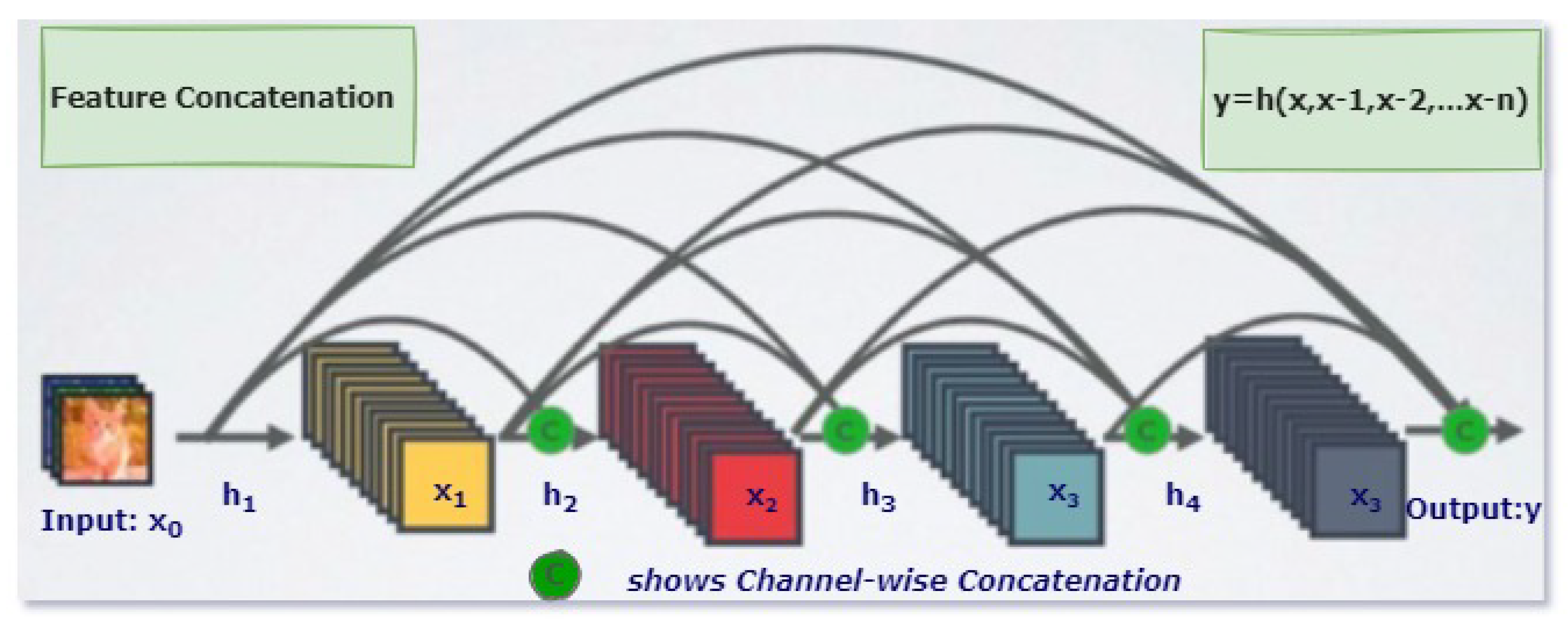
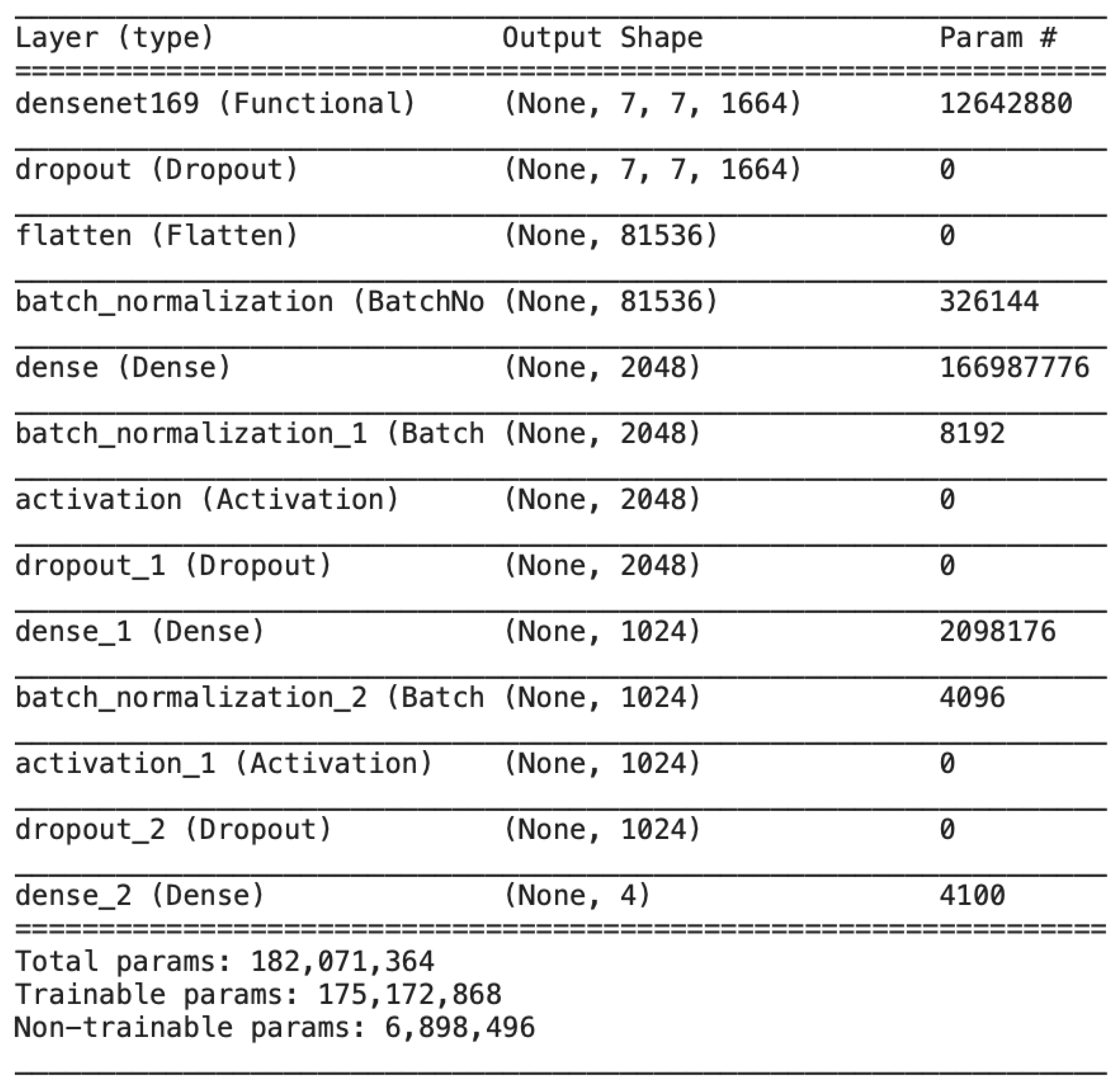
2.4. DenseNet
3. Related Work
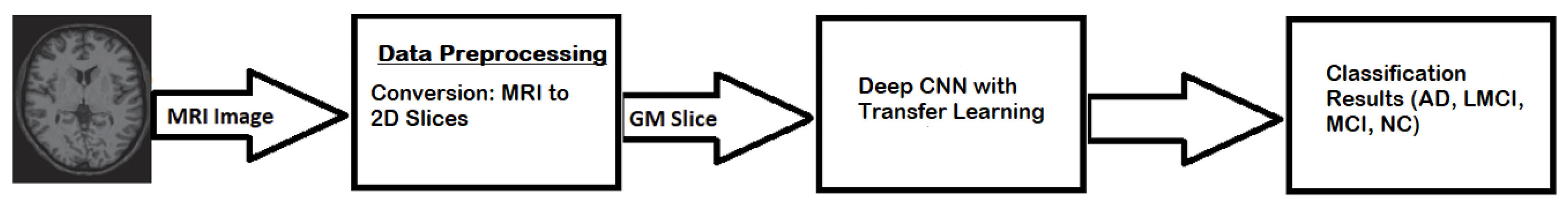
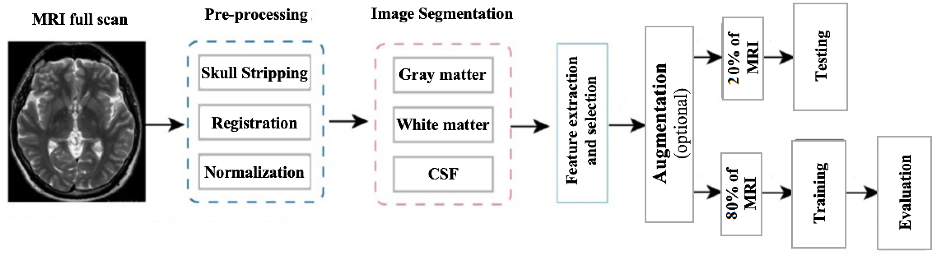
4. Methodology
4.1. DataSet
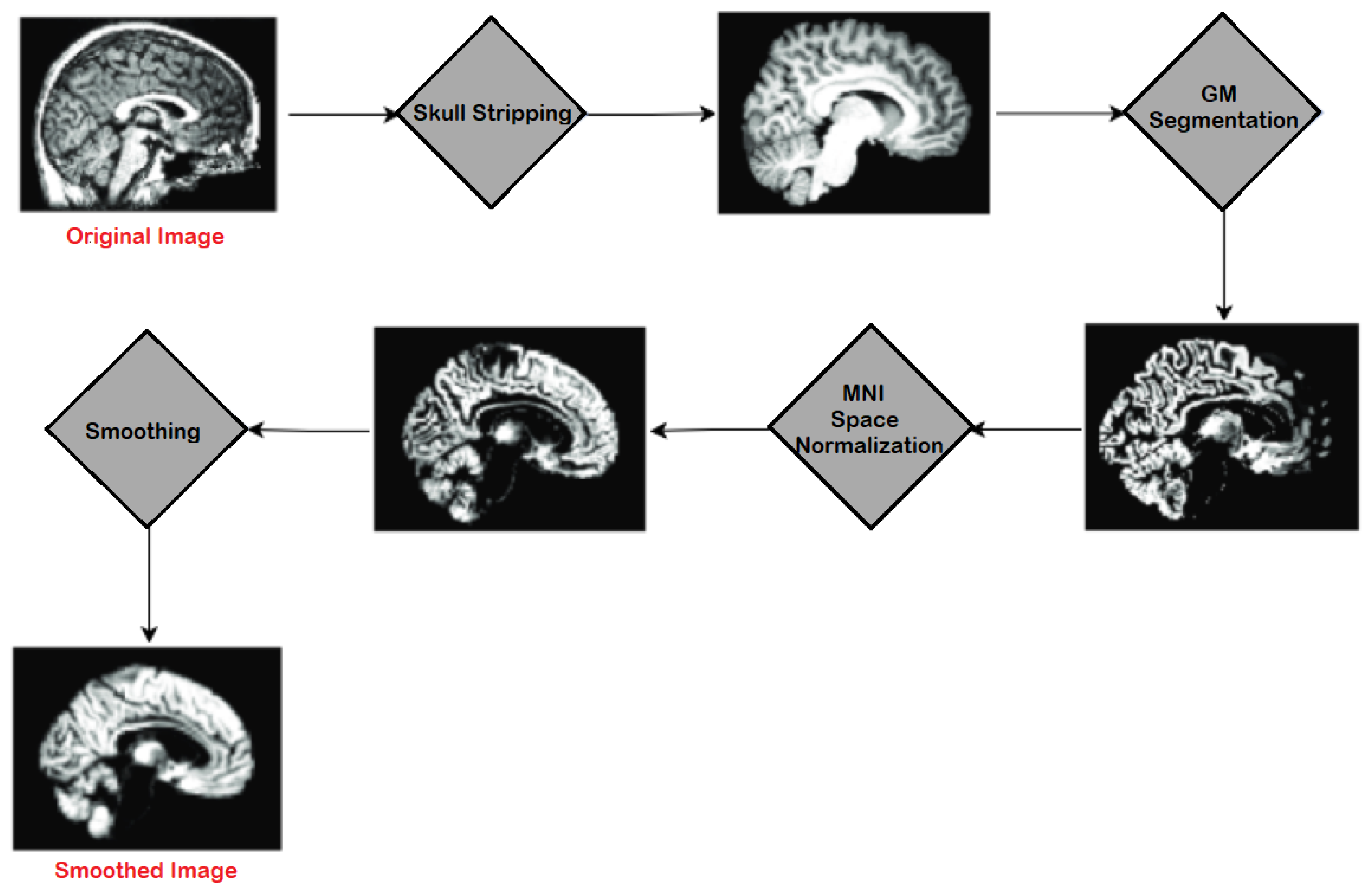
4.2. Data Preprocessing
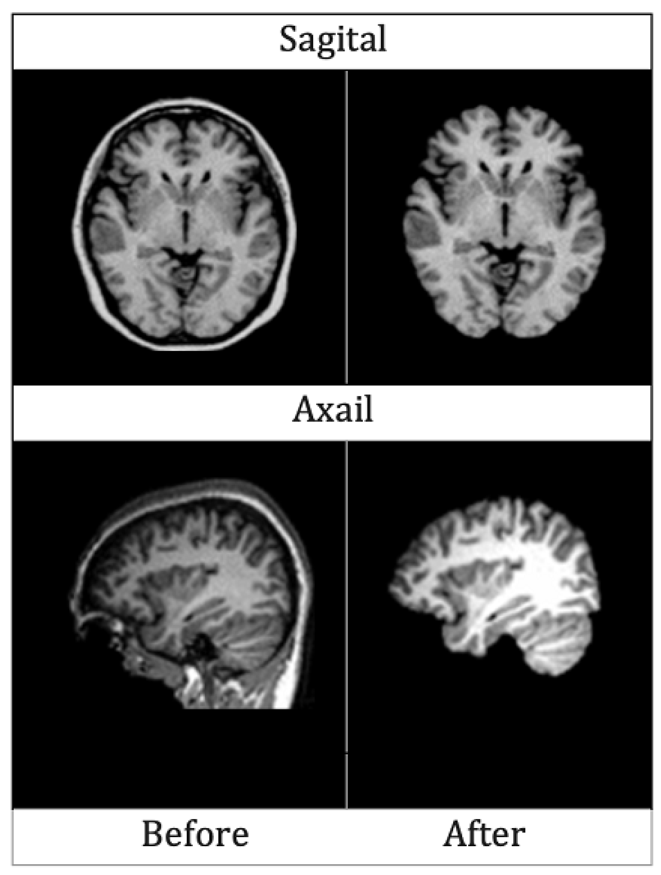
4.2.1. Skull Stripping
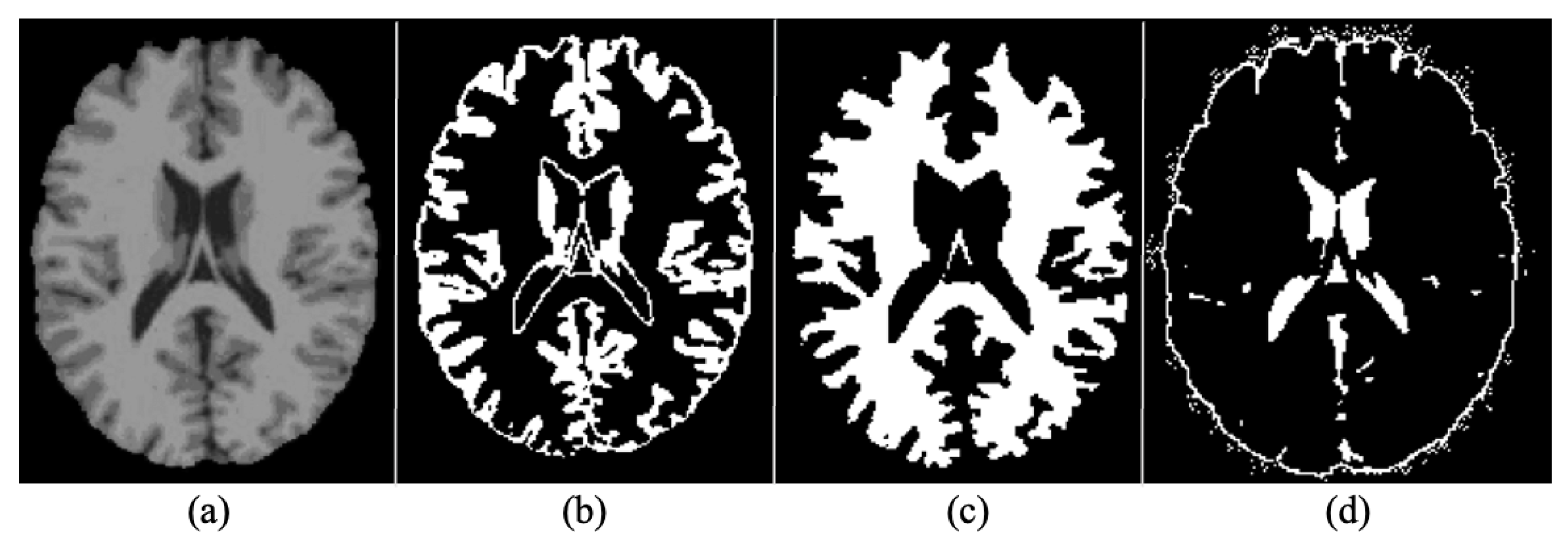
4.2.2. Segmentation
4.2.3. Normalization
4.2.4. Rescaling
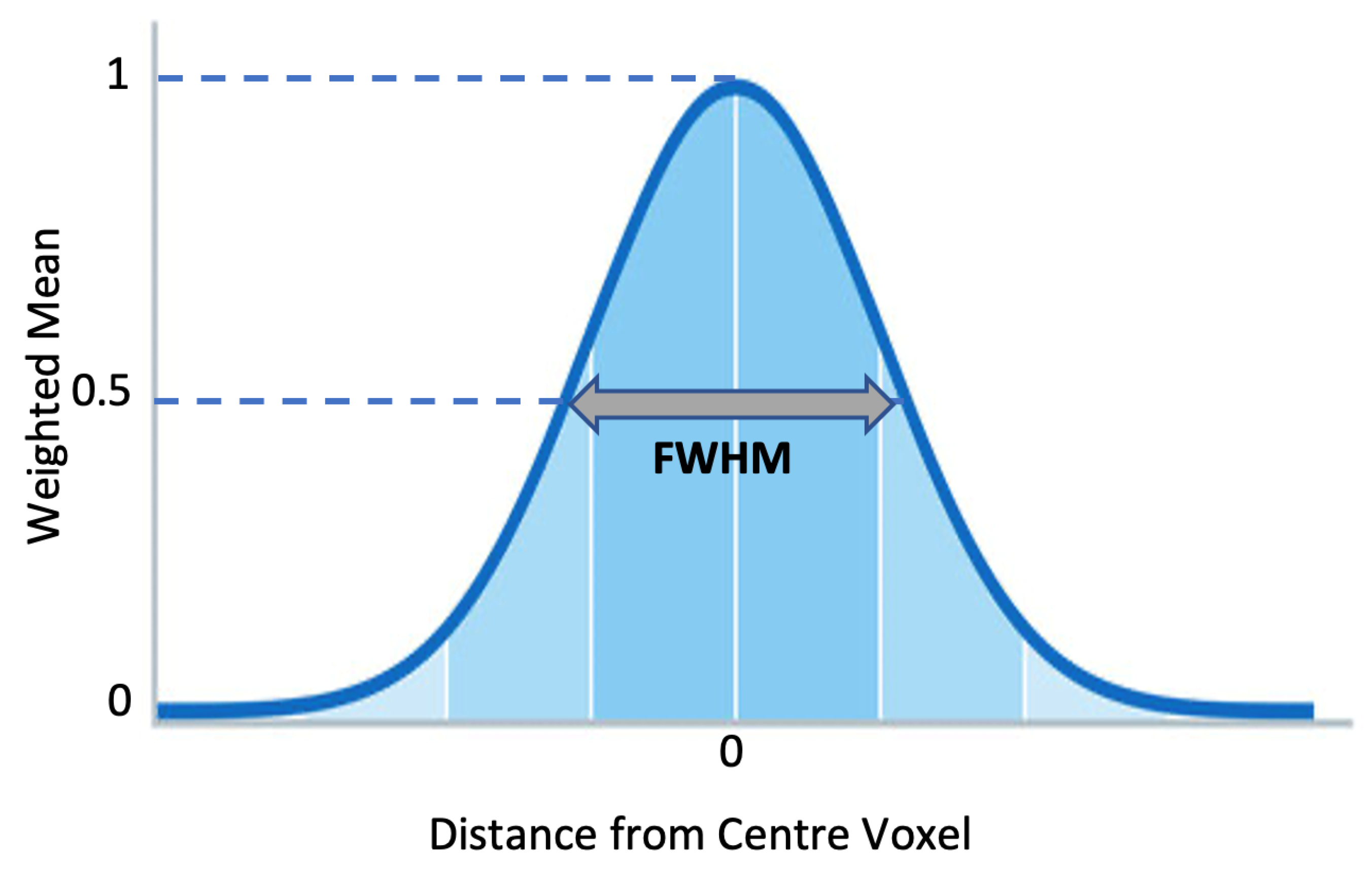
4.2.5. Smoothing
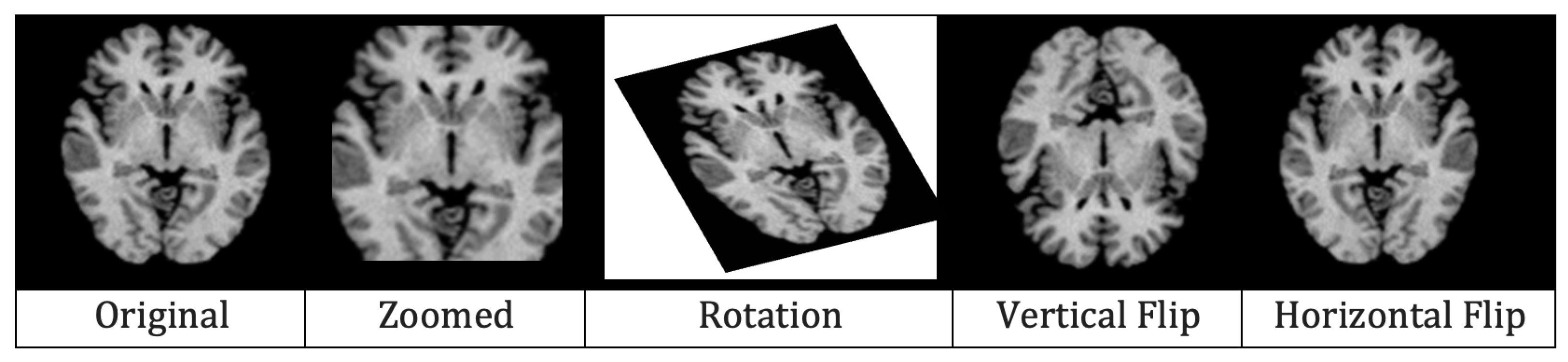
4.2.6. Augmentation
4.3. Architecture
4.4. Experimental Setup and Training
5. Results
6. Discussions
7. Conclusions
Author Contributions
Funding
Data Availability Statement
Acknowledgments
Conflicts of Interest
References
- Srivastava, S.; Ahmad, R.; Khare, S.K. Alzheimer’s disease and its treatment by different approaches: A review. Eur. J. Med. Chem. 2021, 216, 113320. [Google Scholar] [CrossRef] [PubMed]
- Alzheimer’s Association. 2015 Alzheimer’s disease facts and figures. Alzheimer’s Dement. 2015, 11, 332–384. [Google Scholar] [CrossRef] [PubMed]
- Alzheimer’s Association. 2016 Alzheimer’s disease facts and figures. Alzheimer’s Dement. 2016, 12, 459–509. [Google Scholar] [CrossRef] [PubMed]
- Breijyeh, Z.; Karaman, R. Comprehensive review on Alzheimer’s disease: Causes and treatment. Molecules 2020, 25, 5789. [Google Scholar] [CrossRef]
- Jack, C.R., Jr.; Bernstein, M.A.; Fox, N.C.; Thompson, P.; Alexander, G.; Harvey, D.; Borowski, B.; Britson, P.J.; Whitwell, J.L.; Ward, C.; et al. The Alzheimer’s disease neuroimaging initiative (ADNI): MRI methods. J. Magn. Reson. Imaging Off. J. Int. Soc. Magn. Reson. Med. 2008, 27, 685–691. [Google Scholar] [CrossRef]
- Khan, Y.F.; Kaushik, B. Computer vision technique for neuro-image analysis in neurodegenerative diseases: A survey. In Proceedings of the IEEE 2020 International Conference on Emerging Smart Computing and Informatics (ESCI), Pune, India, 9–11 March 2020; pp. 346–350. [Google Scholar]
- Khan, Y.F.; Kaushik, B. Neuro-image classification for the prediction of alzheimer’s disease using machine learning techniques. In Proceedings of the International Conference on Machine Intelligence and Data Science Applications; Springer: Berlin/Heidelberg, Germany, 2021; pp. 483–493. [Google Scholar]
- Ungar, L.; Altmann, A.; Greicius, M.D. Apolipoprotein E, gender, and Alzheimer’s disease: An overlooked, but potent and promising interaction. Brain Imaging Behav. 2014, 8, 262–273. [Google Scholar] [CrossRef]
- Brookmeyer, R.; Johnson, E.; Ziegler-Graham, K.; Arrighi, H.M. Forecasting the global burden of Alzheimer’s disease. Alzheimer’s Dement. 2007, 3, 186–191. [Google Scholar] [CrossRef]
- Naseer, A.; Yasir, T.; Azhar, A.; Shakeel, T.; Zafar, K. Computer-aided brain tumor diagnosis: Performance evaluation of deep learner CNN using augmented brain MRI. Int. J. Biomed. Imaging 2021, 2021, 5513500. [Google Scholar] [CrossRef]
- Kundaram, S.S.; Pathak, K.C. Deep learning-based Alzheimer disease detection. In Proceedings of the 4th International Conference on Microelectronics, Computing And Communication Systems; Springer: Berlin/Heidelberg, Germany, 2021; pp. 587–597. [Google Scholar]
- Naseer, A.; Tamoor, M.; Azhar, A. Computer-aided COVID-19 diagnosis and a comparison of deep learners using augmented CXRs. J. X-ray Sci. Technol. 2021, 30, 1–21. [Google Scholar] [CrossRef]
- Dadar, M.; Manera, A.L.; Ducharme, S.; Collins, D.L. White matter hyperintensities are associated with grey matter atrophy and cognitive decline in Alzheimer’s disease and frontotemporal dementia. Neurobiol. Aging 2022, 111, 54–63. [Google Scholar] [CrossRef]
- Aderghal, K.; Khvostikov, A.; Krylov, A.; Benois-Pineau, J.; Afdel, K.; Catheline, G. Classification of Alzheimer disease on imaging modalities with deep CNNs using cross-modal transfer learning. In Proceedings of the 2018 IEEE 31st International Symposium on Computer-Based Medical Systems (CBMS), Karlstad, Sweden, 18–21 June 2018; pp. 345–350. [Google Scholar]
- Ebrahimi, A.; Luo, S.; Initiative, A.D.N. Disease Neuroimaging Initiative for the Alzheimer’s. Convolutional neural networks for Alzheimer’s disease detection on MRI images. J. Med. Imaging 2021, 8, 024503. [Google Scholar] [CrossRef] [PubMed]
- Farooq, A.; Anwar, S.; Awais, M.; Rehman, S. A deep CNN based multi-class classification of Alzheimer’s disease using MRI. In Proceedings of the 2017 IEEE International Conference on Imaging Systems and Techniques (IST), Beijing, China, 18–20 October 2017; pp. 1–6. [Google Scholar]
- Khedher, L.; Ramírez, J.; Górriz, J.M.; Brahim, A.; Segovia, F.; Alzheimer’s Disease Neuroimaging Initiative. Early diagnosis of Alzheime’s disease based on partial least squares, principal component analysis and support vector machine using segmented MRI images. Neurocomputing 2015, 151, 139–150. [Google Scholar] [CrossRef]
- Plant, C.; Teipel, S.J.; Oswald, A.; Böhm, C.; Meindl, T.; Mourao-Miranda, J.; Bokde, A.W.; Hampel, H.; Ewers, M. Automated detection of brain atrophy patterns based on MRI for the prediction of Alzheimer’s disease. Neuroimage 2010, 50, 162–174. [Google Scholar] [CrossRef] [PubMed]
- Tamoor, M.; Younas, I. Automatic segmentation of medical images using a novel Harris Hawk optimization method and an active contour model. J. X-ray Sci. Technol. 2021, 29, 721–739. [Google Scholar] [CrossRef] [PubMed]
- Malik, Y.S.; Tamoor, M.; Naseer, A.; Wali, A.; Khan, A. Applying an adaptive Otsu-based initialization algorithm to optimize active contour models for skin lesion segmentation. J. X-ray Sci. Technol. 2022, 30, 1–16. [Google Scholar] [CrossRef] [PubMed]
- Gao, M.; Bagci, U.; Lu, L.; Wu, A.; Buty, M.; Shin, H.C.; Roth, H.; Papadakis, G.Z.; Depeursinge, A.; Summers, R.M.; et al. Holistic classification of CT attenuation patterns for interstitial lung diseases via deep convolutional neural networks. Comput. Methods Biomech. Biomed. Eng. Imaging Vis. 2018, 6, 1–6. [Google Scholar] [CrossRef]
- Liu, X.; Wang, C.; Bai, J.; Liao, G. Fine-tuning pre-trained convolutional neural networks for gastric precancerous disease classification on magnification narrow-band imaging images. Neurocomputing 2020, 392, 253–267. [Google Scholar] [CrossRef]
- Naseer, A.; Zafar, K. Meta-feature based few-shot Siamese learning for Urdu optical character recognition. In Computational Intelligence; Wiley: Hoboken, NJ, USA, 2022. [Google Scholar]
- Sezer, A.; Sezer, H.B. Convolutional neural network based diagnosis of bone pathologies of proximal humerus. Neurocomputing 2020, 392, 124–131. [Google Scholar] [CrossRef]
- Kim, H. Organize Everything I Know. 2018. Available online: https://oi.readthedocs.io/en/latest/computer{_}vision/cnn/densenet.html (accessed on 25 November 2022).
- Tsang, S.H. Review: DenseNet—Dense Convolutional Network (Image Classification). 2018. Available online: https://towardsdatascience.com/review-densenet-image-classification-b6631a8ef803 (accessed on 25 November 2022).
- Hon, M.; Khan, N.M. Towards Alzheimer’s disease classification through transfer learning. In Proceedings of the 2017 IEEE International Conference on Bioinformatics and Biomedicine (BIBM), Kansas, MO, USA, 13–16 November 2017; pp. 1166–1169. [Google Scholar]
- Sarraf, S.; Tofighi, G. Deep learning-based pipeline to recognize Alzheimer’s disease using fMRI data. In Proceedings of the IEEE 2016 Future Technologies Conference (FTC), San Francisco, CA, USA, 6–7 December 2016; pp. 816–820. [Google Scholar]
- Liu, S.; Liu, S.; Cai, W.; Che, H.; Pujol, S.; Kikinis, R.; Feng, D.; Fulham, M.J. Multimodal neuroimaging feature learning for multiclass diagnosis of Alzheimer’s disease. IEEE Trans. Biomed. Eng. 2014, 62, 1132–1140. [Google Scholar] [CrossRef]
- Tufail, A.B.; Ma, Y.K.; Zhang, Q.N. Binary classification of Alzheimer’s disease using sMRI imaging modality and deep learning. J. Digit. Imaging 2020, 33, 1073–1090. [Google Scholar] [CrossRef]
- Liu, S.; Liu, S.; Cai, W.; Pujol, S.; Kikinis, R.; Feng, D. Early diagnosis of Alzheimer’s disease with deep learning. In Proceedings of the 2014 IEEE 11th International Symposium on Biomedical Imaging (ISBI), Beijing, China, 29 April–2 May 2014; pp. 1015–1018. [Google Scholar]
- Maqsood, M.; Nazir, F.; Khan, U.; Aadil, F.; Jamal, H.; Mehmood, I.; Song, O.y. Transfer learning assisted classification and detection of Alzheimer’s disease stages using 3D MRI scans. Sensors 2019, 19, 2645. [Google Scholar] [CrossRef] [PubMed]
- Mehmood, A.; Maqsood, M.; Bashir, M.; Shuyuan, Y. A deep Siamese convolution neural network for multi-class classification of Alzheimer disease. Brain Sci. 2020, 10, 84. [Google Scholar] [CrossRef] [PubMed]
- Mehmood, A.; Yang, S.; Feng, Z.; Wang, M.; Ahmad, A.S.; Khan, R.; Maqsood, M.; Yaqub, M. A transfer learning approach for early diagnosis of Alzheimer’s disease on MRI images. Neuroscience 2021, 460, 43–52. [Google Scholar] [CrossRef] [PubMed]
- Qiu, S.; Joshi, P.S.; Miller, M.I.; Xue, C.; Zhou, X.; Karjadi, C.; Chang, G.H.; Joshi, A.S.; Dwyer, B.; Zhu, S.; et al. Development and validation of an interpretable deep learning framework for Alzheimer’s disease classification. Brain 2020, 143, 1920–1933. [Google Scholar] [CrossRef]
- Ramzan, F.; Khan, M.U.G.; Rehmat, A.; Iqbal, S.; Saba, T.; Rehman, A.; Mehmood, Z. A deep learning approach for automated diagnosis and multi-class classification of Alzheimer’s disease stages using resting-state fMRI and residual neural networks. J. Med. Syst. 2020, 44, 1–16. [Google Scholar] [CrossRef]
- Weiner, D.M.W. Alzheimer Disease Neuroimaging Initiative. 2004. Available online: https://adni.loni.usc.edu/ (accessed on 25 November 2022).
- Kalavathi, P.; Prasath, V. Methods on skull stripping of MRI head scan images—A review. J. Digit. Imaging 2016, 29, 365–379. [Google Scholar] [CrossRef]
- Atkins, M.S.; Mackiewich, B.T. Fully automatic segmentation of the brain in MRI. IEEE Trans. Med. Imaging 1998, 17, 98–107. [Google Scholar] [CrossRef]
- Young, J.; Modat, M.; Cardoso, M.J.; Mendelson, A.; Cash, D.; Ourselin, S. Alzheimer’s Disease Neuroimaging Initiative. Accurate multimodal probabilistic prediction of conversion to Alzheimer’s disease in patients with mild cognitive impairment. NeuroImage Clin. 2013, 2, 735–745. [Google Scholar] [CrossRef]
- Ashburner, J.; Friston, K. Voxel-Based Morphometry—The Methods. Neuroimage 2000, 11 Pt 1, 805–821. [Google Scholar] [CrossRef]
- Bose, S.R.; Pearline, A.S.; Bose, R. Real-Time Plant Species Recognition Using Non-Averaged Densenet-169 Deep Learning Paradigm; SSRN: Rochester, NY, USA, 2022. [Google Scholar]
- Vulli, A.; Srinivasu, P.N.; Sashank, M.S.K.; Shafi, J.; Choi, J.; Ijaz, M.F. Fine-Tuned DenseNet-169 for Breast Cancer Metastasis Prediction Using FastAI and 1-Cycle Policy. Sensors 2022, 22, 2988. [Google Scholar] [CrossRef]
- Shanmugam, J.V.; Duraisamy, B.; Simon, B.C.; Bhaskaran, P. Alzheimer’s disease classification using pre-trained deep networks. Biomed. Signal Process. Control 2022, 71, 103217. [Google Scholar] [CrossRef]
- Chamarajan, G.; Charishma, Y.; Ghomi, S.M.T.; Marchiori, E. Alzheimer’s Disease: A Survey. Int. J. Artif. Intell. 2021, 8, 33–39. [Google Scholar]
- Zhou, T.; Ye, X.; Lu, H.; Zheng, X.; Qiu, S.; Liu, Y. Dense Convolutional Network and Its Application in Medical Image Analysis. BioMed Res. Int. 2022, 2022, 2384830. [Google Scholar] [CrossRef] [PubMed]


| HYPERPARAMETERS | |
|---|---|
| Activation Function | ReLU |
| Epochs | 50 |
| Batch Size | 128 |
| Optimizer | Adam |
| Loss Function | Categorical Cross Entropy |
| Drop out | 0.4 |
| Epochs 10 | Epochs 25 | Epochs 50 | |
|---|---|---|---|
| Loss | 6.89% | 3.18% | 2.16% |
| Accuracy | 93.11% | 96.82% | 97.84% |
| Predicted | |||||
|---|---|---|---|---|---|
| MCI | AD | NCI | LMCI | ||
| Actual | MCI | 248 | 1 | 1 | 0 |
| AD | 1 | 247 | 1 | 1 | |
| NCI | 2 | 1 | 247 | 0 | |
| LMCI | 0 | 1 | 0 | 249 | |
| Image Classes | Specificity | Sensitivity | Accuracy |
|---|---|---|---|
| MCI vs. AD, NC and LMCI | 99.89 | 98.42 | 99.52 |
| LMCI vs. AD, NC and MCI | 97.76 | 99.36 | 98.16 |
| NC vs. AD, MCI and LMCI | 99.78 | 94.32 | 98.33 |
| AD vs. NC, MCI and LMCI | 99.69 | 99.65 | 99.68 |
| Transfer Learning | Augmented Data | Accuracy |
|---|---|---|
| No | No | 81.58% |
| No | Yes | 86.04% |
| Yes | No | 93.30% |
| Yes | Yes | 97.84% |
Disclaimer/Publisher’s Note: The statements, opinions and data contained in all publications are solely those of the individual author(s) and contributor(s) and not of MDPI and/or the editor(s). MDPI and/or the editor(s) disclaim responsibility for any injury to people or property resulting from any ideas, methods, instructions or products referred to in the content. |
© 2023 by the authors. Licensee MDPI, Basel, Switzerland. This article is an open access article distributed under the terms and conditions of the Creative Commons Attribution (CC BY) license (https://creativecommons.org/licenses/by/4.0/).
Share and Cite
Raza, N.; Naseer, A.; Tamoor, M.; Zafar, K. Alzheimer Disease Classification through Transfer Learning Approach. Diagnostics 2023, 13, 801. https://doi.org/10.3390/diagnostics13040801
Raza N, Naseer A, Tamoor M, Zafar K. Alzheimer Disease Classification through Transfer Learning Approach. Diagnostics. 2023; 13(4):801. https://doi.org/10.3390/diagnostics13040801
Chicago/Turabian StyleRaza, Noman, Asma Naseer, Maria Tamoor, and Kashif Zafar. 2023. "Alzheimer Disease Classification through Transfer Learning Approach" Diagnostics 13, no. 4: 801. https://doi.org/10.3390/diagnostics13040801
APA StyleRaza, N., Naseer, A., Tamoor, M., & Zafar, K. (2023). Alzheimer Disease Classification through Transfer Learning Approach. Diagnostics, 13(4), 801. https://doi.org/10.3390/diagnostics13040801