Abstract
Age-related macular degeneration is a visual disorder caused by abnormalities in a part of the eye’s retina and is a leading source of blindness. The correct detection, precise location, classification, and diagnosis of choroidal neovascularization (CNV) may be challenging if the lesion is small or if Optical Coherence Tomography (OCT) images are degraded by projection and motion. This paper aims to develop an automated quantification and classification system for CNV in neovascular age-related macular degeneration using OCT angiography images. OCT angiography is a non-invasive imaging tool that visualizes retinal and choroidal physiological and pathological vascularization. The presented system is based on new retinal layers in the OCT image-specific macular diseases feature extractor, including Multi-Size Kernels ξcho-Weighted Median Patterns (MSKξMP). Computer simulations show that the proposed method: (i) outperforms current state-of-the-art methods, including deep learning techniques; and (ii) achieves an overall accuracy of 99% using ten-fold cross-validation on the Duke University dataset and over 96% on the noisy Noor Eye Hospital dataset. In addition, MSKξMP performs well in binary eye disease classifications and is more accurate than recent works in image texture descriptors.
1. Introduction
Age-related macular degeneration is a visual disorder caused by abnormalities in a part of the eye’s retina and is a leading source of visual impairment Ref. [1]. Therefore, early diagnosis and treatment is critical Ref. [2]. Recently, retinal optical coherence tomography (OCT) images have been used to attain information regarding the health of the posterior eye (e.g., the retina and choroid) Ref. [3]. OCT is a quick, non-invasive medical imaging tool that uses low coherence interferometry to produce cross-sectional images of the retina and optic nerve head (ONH), or the most anterior part of the visual pathway, from the retina to lamina the cribrosa, which assess visual disorders, such as optic nerve disease, qualitative and quantitative. High-resolution (in µm range) scanner techniques such as optical coherence tomography (OCT) produce three-dimensional cross-sectional images of the eye’s biological tissues to visualize the individual layers of the posterior segment of the eye, allowing the diagnosis and monitoring of ocular diseases and anomalies Ref. [4]. This development of image acquisition reduces the cost of storage, which allows ophthalmologists to utilize these images to diagnose various eye diseases Refs. [5,6]. However, ophthalmologists would manually interpret each OCT image in the volumes to make a diagnosis decision. The increased data makes manual interpretation of the OCT volumes time-consuming Ref. [7].
Recent research in academia and industry has allowed artificial intelligence, Machine Learning, and Deep Learning (DL) to develop computerized algorithms to classify retinal disorders. These retinal disorders include diabetic macular edema (DME), aged macular degeneration (AMD), and Choroidal Neovascularization (CNV), see Figure 1. DME is the cause of glaucoma, where fluids or glucose build-up within the retinal layer causes vision impairment. Age-related diseases such as Age Macular Degeneration are caused by a build-up of drusen particles within the retinal epithelium layer. Dry AMD, which is usually diagnosed in older individuals, may cause daily life disruptions because it impairs the patient’s central vision. CNV, wet AMD, is when unusual blood vessels grow into the retina layers, causing fluids to leak and making the retina wet. For some people who are diagnosed with AMD, too many vascular blood vessels are produced. These new blood vessels spear from the choroid and then extend into the retina layers. These vessels are also leaky, allowing fluids and blood with red blood cells to enter the retina layers, distorting their vision. For this reason, early diagnosis and automated detection are essential in treating AMD Refs. [6,8,9].
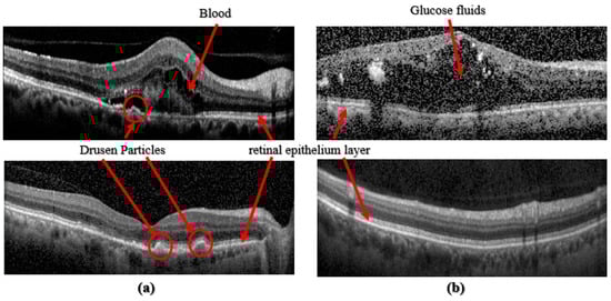
Figure 1.
(a) Images taken from [8], top: CNV class, bottom: Drusen class; (b) Images taken from [9], top: DME class, bottom: Normal class.
The correct detection, precise location, classification, and diagnosis of choroidal neovascularization (CNV) may also be challenging if the lesion is small or if OCT images are degraded by speckle noises. Speckle noises in OCT images must be addressed to achieve good classification performance. Speckle noise, called multiplicative noise, is a granular noise texture. It degrades image quality as a consequence of interference among wavefronts in coherent imaging systems, such as radar, laser imaging, medical ultrasound, and optical coherence tomography. The speckle noise is signal-dependent and governed by the Fisher-Tippett distribution. Mathematically, Speckle noise Refs. [10,11,12,13] is expressed as u(x,y) = v(x,y) + v(x,y)η(x,y), where (x,y) are pixel position, v(x,y) is the clean image, u(x,y) is the noisy image, η is a Gaussian noise distribution with zero-mean and some variance σ2. It is well known that smoothing filters can reduce speckle noise. These techniques convolve an image with various neighbor sizes, 3 × 3, 5 × 5, etc., using a weighted average or selecting a median value, i.e., a non-weighted median filter. However, selecting a median value without any weights from a high noise-density image is not practical because a noise pixel may be selected instead of an image pixel. Therefore, we propose a new texture descriptor, MSKξMP, which echoes or repeats pixel values in a kernel to encode OCT images while avoiding a high level of speckle noises. This paper makes the following contributions:
- -
- Develops a new, simple, and highly accurate local texture descriptor algorithm, Multi-Size Kernels ξcho-Weighted Median Patterns (MSKξMP), to
- (i)
- Avoid speckles noises;
- (ii)
- Perform eye disease classifications the Choroidal Neovascularization and Aged Macular Degeneration;
- (iii)
- Perform highly accurate eye disease classifications between Diabetic Macular Edema, AMD, and Normal eyes.
- -
- Offers a Unique Singular Value Decomposition and Neighborhood Component Analysis based weighted feature selection method for establishing the optimal accuracy using SVM and Random Forest classification techniques.
- -
- Presents computer simulation results that show: (i) 99.78% accuracy on the Duke Dataset, 96.63% and 88.51% on the noisy Noor OCT Volume datasets; (ii) good eye disease diagnosis and recognition outcomes compared to the recent texture descriptors.
This paper has the following structure: the next section contains a Literature Review that offers an overview of methods that give detailed descriptions of the MSKξMP algorithm; the computer simulations section gives numerous experiments showing the performance of MSKξMP; finally, the conclusion and future work are presented in the last section.
2. Literature Review
In recent years, deep learning networks can perform vision recognition in various applications such as self-driving cars, natural language and image processing, and medical diagnosis (e.g., ocular diseases). Ref. [7] proposes an algorithm imitating how ophthalmologists form diagnoses by focusing on the information provided by OCT images during the classification process. This process is called a B-scan attentive convolutional neural network (BACNN). A self-attention module is used to cumulate features based on their clinical importance to obtain feature vectors. Ref. [1] proposes a multipath CNN architecture for the diagnosis of AMD. This architecture has five convolutional layers to classify AMD or normal images.
The multipath convolution layers extract critical global structures with a large filter kernel and use a sigmoid function as the classifier. Ref. [14] presented a CNN based on surrogate-assisted classification that classifies retinal OCT images automatically. Initial preprocessing was performed on each image using image denoising, thresholding, and morphological dilation to locate binary masks of the retina regions. The preprocessed images were employed to produce surrogate images in image augmentation, which were used to train the CNN model.
Several hand-crafted feature techniques show good classification performance on ocular disorder classifications in OCT images. Ref. [4]’s algorithm extracts features using multiscale histograms of oriented gradient descriptors and are classified using a support vector machine. Ref. [15] proposes the automated detection of AMD and DME from retina OCT images based on sparse coding, spatial pyramids, global representations, and dictionary learning. This process is coupled with preprocessing and a support vector machine classifier. Ref. [6] proposed a multiclass model for detecting AMD, DME, and normal using linear configuration patterns (LCPs) to extract pyramid and multiscale features. Recently, [10] proposed a texture descriptor called Alpha Mean Trimmed local binary patterns (AMT-LBP) based on Alpha Mean Trimmed Filter. The AMT-LBP encodes image pixels while partially avoiding and exploiting speckle noises. Table 1 summarizes the rest of the other recent techniques in ocular disorder classification.

Table 1.
Shows prior works and their results.
The current works using hand-crafted features fall short compared to the deep learning technique in achieving extremely high classification accuracies. However, deep-learning models usually require long training times and heavy computational hardware such as GPUs. They are also data-hungry and complex. A simple, aggressive machine-learning approach is proposed here to overcome these shortcomings. This technique contains a smaller number of weights, making them easier to implement, requires less training time, and does not require specialized hardware Ref. [19]. Textural information is vital in analyzing eye diseases. Thus, this paper presents a novel texture descriptor, Multi-Size Kernel ξcho-Weighted Median Patterns, to distinguish between the various ocular diseases while achieving very high classification accuracies.
3. Methods
Our algorithm has the following steps.
- (i)
- Preprocessing: performs image segmentation using thresholding, then flattens and aligns the retina layers;
- (ii)
- Generating Hand-Crafted Features: generating hand-crafted features using Multi-Size Kernels Echo-Weighted Median Patterns (MSKξMP);
- (iii)
- Feature Weights Selection and Classification: best features are selected using Singular Value Decomposition, and neighborhood component analysis (NCA) is classified using Gaussian and Polynomial Kernels Support Machine Vector, Random Forest, Naïve Bayes, Adaboost, and RUS Boost.
3.1. Preprocessing
OCT scanner misalignment between the eye and sensor during the acquisition of the retinal images cause white areas in the image. Therefore, preprocessing Ref. [10] starts with removing white areas by assigning white pixels to black pixels. Then, the image is resized from a square image to a rectangular 256 × 512 image. Next, the image is binarized using Otsu thresholding Ref. [20], which generates a binary image (black and white), and a non-weighted median filter is applied afterward. The purpose of this median filter is not to remove noise in the image but to remove white areas in the binary image outside the retinal regions. A morphological dilated operator with a large structuring element is used on the median filtered image to close fluid region structures in DME and CNV images. Finally, the retinal layers are flattened by applying the polynomial fit of either the 2nd order or 3rd order based on the R2 fitness function. In most cases, the 3rd-order polynomial is selected to flatten the retinal layers.
3.2. Hand-Crafted Features
This section presents new, so-called Multi-Size Kernels ξcho-Weighted Median Patterns (MSKξMP), hand-crafted features. This is an extension of the Local Binary Patterns (LBP) feature extractor [21] and is used in many applications such as texture analysis, face recognition, object detection, fault diagnosis, and image retrieval. The advantages of LBP are that it is computationally simple, efficient, and is invariant to illumination. However, the disadvantages of LBP are its production of artifacts and noises, which distort the central pixel value causing classification degradation. To improve the robustness of LBP, different modifications of LBP were proposed.
In this proposal, we start with the generalized form of the LBP given by the following:
where IC is the center pixel, Ii are the surrounding pixels, f(i) is equal to 2i and R is a region defined by the kernel size. The kernel size is usually selected to be 3 × 3; however, sizes such as 5 × 5 and 7 × 7 are also known to be used. s(Ii − IC) = {1, Ii − IC ≥ T; 0, Ii − IC < T} where T is selected to be zero. The generalized LBP operates on all the pixels in an image using a specific kernel size. Each of these kernels is placed over a pixel, IC, and is compared to its surrounding neighboring pixels Ii using Equation (1). If a neighbor pixel is greater than or equal to the center pixel, then s(·) is assigned 1; if a neighbor pixel is less than the center pixel, then s(·) is assigned 0. A binary sequence is obtained, and each sequence is assigned to the appropriate decimal weight, 2i, which is then converted into a decimal value. The decimal weights, 2i, are then summed and encoded to structural information, generating an LBP image. The LBP is simple, fast, easy, and robust to illumination changes. However, it suffers when speckle noises are present.
The median LBP Ref. [22] was proposed to address these noises. The median LBP can be implemented by replacing IC in (1) with the median value of all the pixels within the region R: IC = Imedian = median(R) = median(I0, I1, I2, … IN−1), where N is the number of pixels in region R. However, the current median LBP does not go far enough to prevent speckle noises from falling into the texture-based calculation. For example, Figure 2a illustrates a 3 × 3 kernel with the following values [135, 75, 75; 135, 75, 75; 160, 135, 135]. The 75’s are image pixels without noise and the 135’s and 160’s are noisy pixels. When we select the median value within the 3 × 3 kernel, we obtain 135, a noisy pixel. To overcome this deficiency, Multi-Size Kernels ξcho-Weighted Median Patterns are proposed.
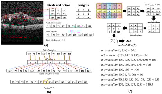
Figure 2.
(a) A noisy DME OCT image taken from [9] with a 3 × 3 kernel of clean and noisy pixels; median is calculated; (b) Finding the median using echo-based weights; (c) A sample calculation of medianLBP5 × 5.
3.3. Multi-Size Kernels Echo-Weighted Median Patterns
MSKξMP is a textural feature descriptor similar to median LBP. MSKξMP encodes the textural pattern information by comparing surrounding pixels to the median pixel Imedian. However, this median value is calculated differently than Ref. [22]. Its surrounding pixels are defined using six different kernel sizes represented using Rn×m, where n’s and m’s have the following values: 3 × 3, 5 × 5, 7 × 7, 3 × 5, 5 × 7, and 3 × 7. Numerous kernel sizes are used because each kernel captures a variation of texture within the OCT; one kernel can miss a specific feature that another kernel size picks up. A larger kernel like the 7 × 7 can capture regional details that a 3 × 3 kernel can miss and vice versa.
The MSKξMP is calculated in three steps for each kernel size, Rn×m. The first is to calculate Imedian, the second is to find each mi’s found in Rn×m, and the third step is to calculate each medianLBPn×m using parameters obtained from steps one and two. The medianLBPn×m is defined by the following equation:
where IC is the current pixel being encoded and is the center pixel of the kernel. The combination of all medianLBPn×m are the MSKξMP. The calculation of Imedian is motivated by the weighted median filter in Ref. [23], which echoes or repeats pixel values a predetermined number of times. Figure 2b illustrates the 3 × 3 kernel, but now echo-weights are applied. The integer of each weight indicates the number of repetitions, e.g., the second element, 75, is repeated two times, or the middle element, 75, is repeated three times. After applying the echo weight to the 3 × 3 kernel, the median was determined to be 75 or Imedian = 75, which is not a noise pixel. These weights can be determined by centering a two-dimensional Gaussian function onto IC, defined by the following:
where σx and σy are standard deviations in the x and y directions, respectively. When a square kernel is utilized, the standard deviations should be the same, σx = σy, and when a rectangular kernel is utilized, the standard deviations could be different, σx ≠ σy. The selection of σx and σy is flexible, as long as the center pixel has the most weight and the surrounding weights are not too small compared to the center. Please see Figure 3, “MSKξMP Weights”. Notice the center weight is only one value higher than its neighboring values. The Gaussian Function is then normalized by its minimum value, min(G(x,y)), to ensure its minimum value equals 1. We then took the ceiling of each element in the normalized Gaussian Function to obtain integer values (or repetition values). The Echo formula can be represented by the following:
where ⌈·⌉ indicates the ceiling operator, and ξ(x,y) represents the echo weights of our kernels. The standard deviations utilized in the 3 × 3 weight kernel, shown in Figure 3, are σx = σy = 1.2. The values of the standard deviations should increase with increasing kernel size. The weight of the center pixel should always have the highest repetition because this gives a non-noise pixel a better chance of being selected as the median.
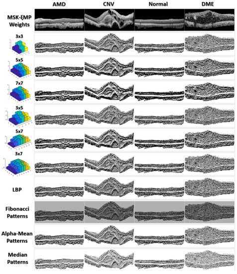
Figure 3.
MSKξMP images associated with their weights, generated using Echo Formula.
Figure 3 shows MSKξMP images associated with their echo weights for all the kernel sizes used in this paper. Notice that the MSKξMP images with weights 5 × 7 and 7 × 7 had the coarsest texture, meaning there were more texture variations and they would provide the highest performance. For example, the MSKξMP of the CNV images can extract drusen particles better than the Fibonacci patterns. The DME image had the most noise, however, the 3 × 3 weighted MSKξMP image could encode less noise compared to the classical LBP.
Finally, Imedian can be written in terms the pixel intensities in Rn×m:
where △ is a duplication operator, ε0, ε1, … εN−1 are elements in the matrix ξ(x,y) and Ii, i = 0, 1, …, N − 1 are the pixel values in Rn×m. reads the following: I0 is duplicated ε0 number of times.
The second step is to determine mi values. These median values are selected within sub-regions of Rn×m and are color-coded in red, yellow, and blue, see top of Figure 4. The pair of regions to the left and right of the center pixel are coded in yellow, the corner sub-regions are coded in red, and the top and bottom sub-regions are coded in blue. A sample calculation of mi’s within a 5 × 5 kernel is illustrated in the following. East (yellow): m1 = median(0, 135) = 67.5, northeast (red): m2 = median(123, 147, 0, 135) = 106; north (blue): m3 = median(106, 123, 123, 106, 0, 0) = 106; northwest (Red): m4 = median(106, 106, 106, 106) = 106; West (yellow): m5 = median(106, 106) = 106; southwest (red): m6 = median(70, 70, 70, 70) = 70; south (blue): m7 = median(70, 153, 153, 70, 153, 153) = 153; and southeast (red): m8 = median(153, 128, 153, 128) = 140.5.
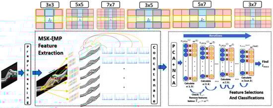
Figure 4.
MSKξMP OCT Image recognition system.
Once all the mi’s are calculated, we moved to the third step, where we compared mi’s to Imedian found in the first step using (2). The comparison encoded the mi’s to binaries which were then multiplied by their respective decimal weights, and the sum was calculated to obtain medianLBP5 × 5(IC). The rest of the medianLBPn×m’s are obtained similarly. Figure 3 shows that each medianLBPn×m image displays different textural information, which is beneficial in distinguishing the different types of ocular disorders.
Four histograms were generated for each medianLBPn×m image to extract their features. One histogram was generated from the entire medianLBPn×m image, which represented the global features. The other three histograms were generated from local overlapping regions and labeled with different color brackets, as seen in Figure 4. Each local regions had a size of 256 × 256 to capture local features. The four histograms from each medianLBPn×m are concatenated to form the MSKξMP feature vector for each OCT image.
4. Computer Simulation
4.1. Datasets
Three datasets were used to test the performance of MSKξMP. The first dataset, designated as Dataset 1, was taken from Duke University, Harvard University, and the University of Michigan Ref. [4]. This dataset consisted of SD-OCT volumetric scans acquired from 45 patients: 15 normal patients, 15 patients with dry AMD, and 15 patients with DME. All SD-OCT volumes were acquired in Institutional Review Board-approved protocols using Spectralis SD-OCT (Heidelberg Engineering Inc., Heidelberg, Germany). The second dataset, which will be designated as Dataset 2, was acquired from the Noor Eye Hospital dataset Ref. [9] and consisted of 148 SD-OCT volumes (48 AMD, 50 DME, and 50 Normal), acquired by using the Heidelberg SD-OCT imaging system at Noor Eye Hospital in Tehran (NEH). Each volume consisted of 19 to 61 B-scans; the resolution of the B-scans was 3.5 μm, and the scan dimension was 8.9 × 7.4 mm2.
The third dataset, Dataset 3, was also collected by the Heidelberg SD-OCT imaging system at Noor Eye Hospital (NEH) and was obtained from the Mendeley database website Ref. [8]. It contained 16,822 OCTs images of Normal (120 volumes), Drusen (160 volumes), and CNV (161 volumes). However, 12,641 images (3234 CNV, 3740 Drusen, and 5667 Normals) were selected for our experiments. This is because we were only keeping worst-case condition images for each volume, whereas if a patient was labeled a CNV case, only CNV B-scans within that volume were included for training and testing procedures. Normal and drusen B-scans of that patient were excluded. Note that drusen particles are early signs of aged macular degeneration, which can be treated in the same class as AMD.
4.2. Feature Weightings, Selection, and Classification
Principal Component Analysis (PCA) is one of the oldest and most widely used statistical techniques that reduces feature dimensionalities. PCA improves interpretability while preserving variability, which minimizes informational loss. This means finding new variables Fi that are linear functions of those in the original features, while successively maximizing variance and maintaining uncorrelatability. This allows the representation of a class of features in the following form:
where λi eigenvalues are sorted according to the size as λ1 ≥ λ2 ≥ … ≥ λp ≥ 0, Fi, i = 1, 2, … p, features, F1 is the best feature and the 2nd, 3rd, …, kth (k ≥ 4) are other principal components.
The PCA used in this paper was based on Singular Value Decomposition (SVD), which was used to select our best features. X = UΣVT represents the SVD of an input matrix X, where U represents the reflection of X, the diagonal of Σ represents the variabilities, σ1, …, ση, up to the η-th feature, VT is the ‘eigen vectors’ of X. X will be subtracted by its mean of each column of Xmean, to obtain Xm = X − Xmean. This subtraction is commonly used for normalizing PCA data. We then calculated XPCA, which is defined by the following:
where M is selected based on the percentage of variability up to η, η ≥ M, N is the number of total observations in the dataset and the dimensions of XPCA is N rows by M columns.
Our feature selection also included feature weighting using neighborhood component analysis (NCA) Ref. [24] to refine our feature searching process. NCA is a feature weighting algorithm utilizing the nearest neighbor to maximize expected leave-one-out classification accuracy. Then NCA was optimized using stochastic gradient accent to learn a feature weighting vector. The output of the NCA is a vector, ω, of length of η representing the weight importance of each feature. Each element in ω is assigned to each column of matrix XPCA.
We then searched for sets of optimal features by reducing the number of columns of XPCA through iterations. The values of the weights in ω were used for removing features from XPCA at iteration. The weights can be written as the following:
where Ml, is the number of features remaining after some features have been removed at lth iteration. This idea was taken from Ref. [25] “Drop Out”, where a Neural Network with a large number of parameters tended to overfit a dataset, causing a decrease in performance. The function of dropout is to drop neuron units with low weights from the neural network during training after multiplying feature weights to feature vectors. Our algorithm utilized this idea to drop features with weights that were below a certain threshold. By dropping these unimportant features, we achieved faster training times and prevented overfitting. To multiply feature weights to feature vectors, ω can be rewritten in matrix form by replicating each element and putting them in column wise fashion. Ω(l) is defined by the following:
where Ω has N number of rows. We can rewrite our input classification matrix, XPCA(l), in terms of Ω and at lth iteration using the following:
where is the feature vector in the ith row of , “” indicates point matrix multiplication operation, is the weight removal threshold at lth iteration, and is the updated feature matrix with M1 number of features. The features that are dropped have feature weights below at the l iteration. XPCA(l) is a new classification input matrix and is inputted to each of the classifiers. The classifiers used during each iteration are RUS-Boost Ref. [26], and Naïve Bayes Ref. [27] and support vector machine using Polynomial and Gaussian Ref. [28], Random Forest Ref. [29] and Adaboost Ref. [30]. values selected for this paper ranged from 0.1 to 1 with increments of 0.01. The classification accuracies, a(l,k), were recorded in each lth iteration at the kth classifier. a(l,k) was defined by the following:
where Ck was one of the kth classifiers listed above. The maximum accuracy was found using the following:
where argmax(·) determines the maximum location or accuracy of lth at kth classifier. Dataset 1, 2, and 3 were trained in this fashion. The η was selected to be 100 for Dataset 1, and 70 for Dataset 2 and 3. Figure 4 shows the MSKξMP OCT Image recognition system from start to finish.
4.3. Performance Evaluation
To evaluate and determine the performance of the proposed feature extraction approach, the accuracy, sensitivity, specificity, precision, and F1-score were compared with the results of HOG Ref. [4], BACNN Ref. [7], Alpha Mean Trimmed Patterns Ref. [10], Fibonacci Patterns Ref. [19], Classical LBP Ref. [21], Vision Transformer Ref. [31], ResNet Ref. [32], VGG16 Ref. [33], and Inception V3 Ref. [34]. By definition, higher values on these indexes imply better quality measures of classification. Mathematical formulas of these measurements are given below:
where Tp and Tn are the true positive and true negative and Fp and Fn are the false positive and false negative, respectively.
5. Results and Discussions
For datasets 1 and 2, four different classification schemes were tested using MSKξMP, AMD vs. DME vs. Normal, AMD vs. DME, DME vs. Normal, Normal vs. AMD, and all classes. Since dataset 1 was slightly imbalanced, AMD (723 images), DME (1101), and has Normal (1407), using accuracy as the only measurement would not be enough to detail the efficacies of the MSKξMP. Using measurements such as recall, specificity, precision, and F1-score was more effective. For dataset 3, we also tested using four classification schemes: Normal vs. CNV, CNV vs. Drusen, Normal vs. Drusen, and all classes, Normal vs. CNV vs. Drusen. Our experiments included kernel sizes up to 3 × 9 and 5 × 9, however, these window sizes were too large, and important features detected may not be within the local areas of the pixel, IC. Therefore, kernel sizes up to n × 9 were omitted from the result section. As using more kernels with varying sizes would have diminishing returns and performance improvements would be minimal. Using six kernels is the right balance between computation times and performances of our MSKξMP.
5.1. Dataset 1, 2 and 3 Results
The highlights of our experiments on datasets 1 and 2 are shown in Table 2 and Figure 5, which show the performance measurements of our MSKξMP. The highest accuracy was achieved by SVM using polynomial kernel at 99.78% on dataset 1 and 96.59% on dataset 2. We achieved 100% on some of the binary classifications, Normal vs. AMD and Normal vs. DME, both using SVM with polynomials as well. Rus-Boost and Naïve Bayes seem to perform the worst, while Adaboost and Random Forest have similar performance to each other. This is because Adaboost and Random Forest both utilize an ensemble of weaker classifiers to create one stronger classifier: K-nearest-neighbor Classifiers to create Adaboost and decision trees for creating Random Forest. The highest accuracy was achieved by SMV polynomial. Regarding misclassifications, SVM polynomial kernel did not misclassify any normal images, only misclassified two DME class images, and using SVM Gaussian only two DME images are misclassified for dataset 1, see confusion matrixes Figure 5. Something to note on dataset 2’s results are their sensitivities (recall) and specificity, notice the specificity was 98.33%, which is higher than the accuracy and sensitivity; this suggests high confidence in their true negatives.
Table 2.
Results from datasets 1, 2 and 3.
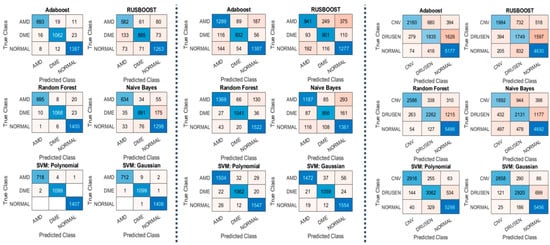
Figure 5.
(Left) Confusion Matrixes from Dataset 1; (Middle) Confusion Matrixes from Dataset 2; (Right) Confusion Matrixes from Dataset 3.
The main takeaway from the results in dataset 3 is that our MSKξMP was able to achieve 89.3% in accuracy using SVM polynomial kernel with specificity of 94.37%. This means high confidences in the true negative diagnoses. The other classifiers performed similarly to dataset 1 and dataset 2. Normal vs. CNV achieved the highest accuracy at 98.53% due to the significant differences between their visual features. It can be observed that MSKξMP was able to achieve 93.69% accuracy with the CNV vs. Drusen classification scheme. This is a good score because while CNV images contain drusen particles that may cause some confusion with AMD images, our feature extractor was able to differentiate between these two classes reliably.
Figure 6 shows ROC curves for our best results “SVM: Polynomial” in all three datasets. For each dataset, we plotted three ROC curves with one class being the positive class of the other two classes. For example, dataset 1 have three classes: Normal, DME, and AMD. One curve plots the True Positives vs. the False Positives using Normal as the positive class and DME and AMD as the negative classes. The area under the curves (AUC) are also computed for each respective curve. Notice the AUCs for dataset 1 were higher and the AUCs of dataset 3 were lower, which reflects their respective accuracies, sensitivities, and specificity.
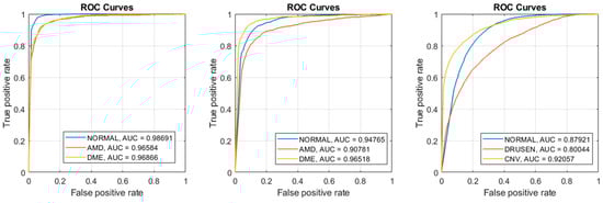
Figure 6.
SVM: Poly produced the best results (Left) ROC curves of Dataset 1; (Middle) ROC curves of Dataset 2; (Right) ROC curves of Dataset 3.
5.2. Ablation Study
For our ablation study, we tested the feature extraction capabilities of each kernel size and weights (shown in Figure 3) on dataset 1. From Table 3, it can be observed that the accuracies measured were highest with the 5 × 7 and 7 × 7 kernels. For each kernel size, the accuracies were about 0.5–3% below our highest achieved accuracy of 99.78% (all kernels). Concatenating the feature vectors generated from each kernel size helped improve the performances of our MSKξMP and indicated that each sized kernel captured different textural information from the OCT image, both locally and regionally. Based on this ablation study, we decided to omit the 3 × 3 kernel and test combined features generated by 5 × 5, 7 × 7, 3 × 5, 5 × 7 and 3 × 7. We were able to achieve an accuracy of 99.78% by SVM polynomial kernel without using the 3 × 3 kernel.
Table 3.
Results of ablation study.
5.3. Comparisons to Recent State of the Art
Comparing dataset 1 with recent state of the art shows our MSKξMP is able to achieve slightly higher accuracies, as shown in Table 4 and Table 5. Das Ref. [7]’s BACNN achieved an accuracy of 97.76% with a plus or minus of 2.24%, meaning BACNN was able to achieve 100% but with extremely high fluctuation. Even though our experiments were based on ten-fold validations, our fluctuation was only about 0.3–0.4%, which is more stable than BACNN. Compared to other state of the arts, our MSKξMP outperformed very deep CNNs such as Refs. [13,32,34] as well as the recent discovery of vision transformer algorithm Ref. [31]. Also, our MSKξMP was able to outperform recent state of the art texture descriptors such as Refs. [10,19], by 99.78% to 94.96% and 99.16% respectively, see Table 6. Table 7 shows datasets 2 and 3 comparisons between the recent state of the art and our MSKξMP. Our accuracies either outperformed or were comparable against deep learning techniques such as Ref. [35]. Note that Ref. [35] had high fluctuations across all performance measurements, ±0.8–3%, whereas our results with MSKξMP only fluctuated within 0.1–0.2%.
Table 4.
Dataset 1 comparisons to recent state of the art.
Table 5.
Dataset 1 comparisons to recent state of the art.
Table 6.
Dataset 1 comparisons to recent texture descriptors.
Table 7.
Dataset 2 and 3 comparisons to recent state of the art.
6. Conclusions and Future Work
This work presents a new image textural descriptor, MSKξMP, for differentiating between ocular diseases such as AMD, Drusen, DME, and CNV in OCT images. The presented method can be used to encode textural patterns at local and regional scales and to improve edges in various directions while avoiding speckle noises. The computer simulations show that our measurements outperformed (a) the current state-of-the-art deep learning techniques and vision transformer; and (b) the FPN-EfficientNetB0 in dataset 3 and is comparable to the FPN-ResNet50 network. Some of our binary classifications from dataset 1 also performed well, achieving perfect accuracy, or close to it. MSKξMP had high specificity, suggesting high confidence in their true negatives. Future work should be focused on constructing 3D retinal images, such as 3D OCT images, by extracting volume and depth information to determine the spread of the disease. The 3D structures should be used for multi-view classification.
Author Contributions
A.L. and S.A., methodology; A.L., validation; A.L. and S.A., formal analysis, investigation; A.L. and S.A., data generation; A.L. and S.B., writing—original draft preparation; S.A. and S.B.; writing—review and editing. All authors have read and agreed to the published version of the manuscript.
Funding
This research received no external funding.
Informed Consent Statement
Not applicable.
Data Availability Statement
Duke Dataset is found here: https://people.duke.edu/~sf59/Srinivasan_BOE_2014_dataset.htm, NOOR datasets are found here: https://hrabbani.site123.me/available-datasets/dataset-for-oct-classification-50-normal-48-amd-50-dme and https://data.mendeley.com/datasets/8kt969dhx6/1 (accessed on 1 January 2020).
Acknowledgments
We would like to thank Anna Liew for assisting us in understanding and analyzing the OCT image features.
Conflicts of Interest
The authors declare no conflict of interest.
References
- Thomas, A.; Harikrishnan, P.M.; Krishna, A.K.; Palanisamy, P.; Gopi, V.P. Automated Detection of Age-Related Macular Degeneration from OCT Images Using Multipath CNN. J. Comput. Sci. Eng. 2021, 15, 34–46. [Google Scholar] [CrossRef]
- Bhende, M.; Shetty, S.; Parthasarathy, M.K.; Ramya, S. Optical coherence tomography: A guide to interpretation of common macular diseases. Indian J. Ophthalmol. 2018, 66, 20–35. [Google Scholar] [CrossRef]
- Thomas, A.; Harikrishnan, P.; Ramachandran, R.; Ramachandran, S.; Manoj, R.; Palanisamy, P.; Gopi, V.P. A novel multiscale and multipath convolutional neural network based age-related macular degeneration detection using OCT images. Comput. Methods Programs Biomed. 2021, 209, 106294. [Google Scholar] [CrossRef]
- Srinivasan, P.P.; Kim, L.A.; Mettu, P.S.; Cousins, S.W.; Comer, G.M.; Izatt, J.A.; Farsiu, S. Fully automated detection of diabetic macular edema and dry age-related macular degeneration from optical coherence tomography images. Biomed. Opt. Express 2014, 5, 3568–3577. [Google Scholar] [CrossRef]
- Fujimoto, J.G.; Pitris, C.; Boppart, S.A.; Brezinski, M.E. Optical Coherence Tomography: An Emerging Technology for Biomedical Imaging and Optical Biopsy. Neoplasia 2000, 2, 9–25. [Google Scholar] [CrossRef]
- Drexler, W.; Fujimoto, J. Optical Coherence Tomography: Technology and Applications; Springer: Berlin/Heidelberg, Germany, 2008. [Google Scholar]
- Das, V.; Prabhakararao, E.; Dandapat, S.; Bora, P.K. B-Scan Attentive CNN for the Classification of Retinal Optical Coherence Tomography Volumes. IEEE Signal Process. Lett. 2020, 27, 1025–1029. [Google Scholar] [CrossRef]
- Sotoudeh-Paima, S. Labeled Retinal Optical Coherence Tomography Dataset for Classification of Normal, Drusen, and CNV Cases, Mendeley Data, 2021, V1. Available online: https://paperswithcode.com/dataset/labeled-retinal-optical-coherence-tomography (accessed on 4 January 2023).
- Rasti, R.; Rabbani, H.; Mehridehnavi, A.; Hajizadeh, F. Macular OCT Classification Using a Multiscale Convolutional Neural Network Ensemble. IEEE Trans. Med Imaging 2017, 37, 1024–1034. [Google Scholar] [CrossRef] [PubMed]
- Liew, A.; Ryan, L.; Agaian, S.S. Alpha mean trim texture descriptors for optical coherence tomography eye classification. Multimodal Image Exploit. Learn. 2022, 12100, 157–167. [Google Scholar] [CrossRef]
- Szkulmowski, M.; Gorczynska, I.; Szlag, D.; Sylwestrzak, M.; Kowalczyk, A.; Wojtkowski, M. Efficient reduction of speckle noise in Optical Coherence Tomography. Opt. Express 2012, 20, 1337–1359. [Google Scholar] [CrossRef]
- Choi, H.; Jeong, J. Speckle Noise Reduction Technique for SAR Images Using Statistical Characteristics of Speckle Noise and Discrete Wavelet Transform. Remote Sens. 2019, 11, 1184. [Google Scholar] [CrossRef]
- Yu, H.; Ding, M.; Zhang, X.; Wu, J. PCANet based non-local means method for speckle noise removal in ultrasound images. PLoS ONE 2018, 13, e0205390. [Google Scholar] [CrossRef] [PubMed]
- Rong, Y.; Xiang, D.; Zhu, W.; Yu, K.; Shi, F.; Fan, Z.; Chen, X. Surrogate-Assisted Retinal OCT Image Classification Based on Convolutional Neural Networks. IEEE J. Biomed. Health Inform. 2018, 23, 253–263. [Google Scholar] [CrossRef] [PubMed]
- Sun, Y.; Li, S.; Sun, Z. Fully automated macular pathology detection in retina optical coherence tomography images using sparse coding and dictionary learning. J. Biomed. Opt. 2017, 22, 016012. [Google Scholar] [CrossRef] [PubMed]
- Wang, Y.; Zhang, Y.; Yao, Z.; Zhao, R.; Zhou, F. Machine learning based detection of age-related macular degeneration (AMD) and diabetic macular edema (DME) from optical coherence tomography (OCT) images. Biomed. Opt. Express 2016, 7, 4928–4940. [Google Scholar] [CrossRef] [PubMed]
- Hussain, M.; Bhuiyan, A.; Luu, C.D.; Smith, R.T.; Guymer, R.H.; Ishikawa, H.; Schuman, J.S.; Ramamohanarao, K. Classification of healthy and diseased retina using SD-OCT imaging and Random Forest algorithm. PLoS ONE 2018, 13, e0198281. [Google Scholar] [CrossRef]
- Wang, D.; Wang, L. On OCT Image Classification via Deep Learning. IEEE Photonics J. 2019, 11, 3900714. [Google Scholar] [CrossRef]
- Panetta, K.; Sanghavi, F.; Agaian, S.; Madan, N. Automated Detection of COVID-19 Cases on Radiographs using Shape-Dependent Fibonaccip Patterns. IEEE J. Biomed. Health Inform. 2021, 25, 1852–1863. [Google Scholar] [CrossRef]
- Otsu, N. A threshold selection method from gray-level histograms. IEEE Trans. Syst. Man Cybern. 1979, 9, 62–66. [Google Scholar] [CrossRef]
- Morales, S.; Engan, K.; Naranjo, V.; Colomer, A. Retinal Disease Screening through Local Binary Patterns. IEEE J. Biomed. Health Inform. 2015, 21, 184–192. [Google Scholar] [CrossRef]
- Hafiane, A.; Seetharaman, G.; Zavidovique, B. Median Binary Pattern for Textures Classification. In Proceedings of the International Conference Image Analysis and Recognition, Montreal, QC, Canada, 22–24 August 2007; pp. 387–398. [Google Scholar] [CrossRef]
- Zhang, Q.; Xu, L.; Jia, J. 100+ Times Faster Weighted Median Filter. In Proceedings of the 2014 IEEE Conference on Computer Vision and Pattern Recognition, Columbus, OH, USA, 23–28 June 2014. [Google Scholar]
- Yang, W.; Wang, K.; Zuo, W. Neighborhood Component Feature Selection for High-Dimensional Data. J. Comput. 2012, 7, 161–168. [Google Scholar] [CrossRef]
- Srivastava, N.; Hinton, G.; Krizhevsky, A.; Sutskever, I.; Salakhutdinov, R. Dropout: A Simple Way to Prevent Neural Networks from Overfitting. J. Mach. Learn. Res. 2014, 15, 1929–1958. [Google Scholar]
- Friedman, J.H. Greedy function approximation: A gradient boosting machine. Ann. Stat. 2001, 29, 1189–1232. [Google Scholar] [CrossRef]
- Manning, C.D.; Raghavan, P.; Schütze, M. Introduction to Information Retrieval; Cambridge University Press: Cambridge, UK, 2008. [Google Scholar]
- Christianini, N.; Shawe-Taylor, J. An Introduction to Support Vector Machines and Other Kernel-Based Learning Methods; Cambridge University Press: Cambridge, UK, 2000. [Google Scholar]
- Breiman, L. Random Forests. Mach. Learn. 2001, 45, 5–32. [Google Scholar] [CrossRef]
- Freund, Y.; Schapire, R.E. A Decision-Theoretic Generalization of On-Line Learning and an Application to Boosting. J. Comput. Syst. Sci. 1997, 55, 119–139. [Google Scholar] [CrossRef]
- Jiang, Z.; Wang, L.; Wu, Q.; Shao, Y.; Shen, M.; Jiang, W.; Dai, C. Computer-aided diagnosis of retinopathy based on vision transformer. J. Innov. Opt. Health Sci. 2022, 15, 2250009. [Google Scholar] [CrossRef]
- He, K.; Zhang, X.; Ren, S.; Sun, J. Deep residual learning for image recognition. In Proceedings of the IEEE Computer Society Conference on Computer Vision and Pattern Recognition (CVPR), Las Vegas, NV, USA, 27–30 June 2016; pp. 770–778. [Google Scholar] [CrossRef]
- Simonyan, K.; Zisserman, A. Very deep convolutional networks for large-scale image recognition. arXiv 2014, arXiv:1409.1556. [Google Scholar]
- Szegedy, C.; Vanhoucke, V.; Ioffe, S.; Shlens, J.; Wojna, Z. Rethinking the Inception Architecture for Computer Vision. In Proceedings of the IEEE Conference on Computer Vision and Pattern Recognition (CVPR), Las Vegas, NV, USA, 27–30 June 2016; pp. 2818–2826. [Google Scholar] [CrossRef]
- Sotoudeh-Paima, S.; Jodeiri, A.; Hajizadeh, F.; Soltanian-Zadeh, H. Multiscale convolutional neural network for automated AMD classification using retinal OCT images. Comput. Biol. Med. 2022, 144, 105368. [Google Scholar] [CrossRef]
- Luo, Y.; Xu, Q.; Jin, R.; Wu, M.; Liu, L. Automatic detection of retinopathy with optical coherence tomography images via a semi-supervised deep learning method. Biomed. Opt. Express 2021, 12, 2684–2702. [Google Scholar] [CrossRef]
- Mousavi, E.; Kafieh, R.; Rabbani, H. Classification of dry age-related macular degeneration and diabetic macular oedema from optical coherence tomography images using dictionary learning. IET Image Process 2020, 14, 1571–1579. [Google Scholar] [CrossRef]
- Karri, S.P.K.; Chakraborty, D.; Chatterjee, J. Transfer learning based classification of optical coherence tomography images with diabetic macular edema and dry age-related macular degeneration. Biomed. Opt. Express 2017, 8, 579–592. [Google Scholar] [CrossRef]


Disclaimer/Publisher’s Note: The statements, opinions and data contained in all publications are solely those of the individual author(s) and contributor(s) and not of MDPI and/or the editor(s). MDPI and/or the editor(s) disclaim responsibility for any injury to people or property resulting from any ideas, methods, instructions or products referred to in the content. |
© 2023 by the authors. Licensee MDPI, Basel, Switzerland. This article is an open access article distributed under the terms and conditions of the Creative Commons Attribution (CC BY) license (https://creativecommons.org/licenses/by/4.0/).