Abstract
Skin Cancer (SC) is among the most hazardous due to its high mortality rate. Therefore, early detection of this disease would be very helpful in the treatment process. Multilevel Thresholding (MLT) is widely used for extracting regions of interest from medical images. Therefore, this paper utilizes the recent Coronavirus Disease Optimization Algorithm (COVIDOA) to address the MLT issue of SC images utilizing the hybridization of Otsu, Kapur, and Tsallis as fitness functions. Various SC images are utilized to validate the performance of the proposed algorithm. The proposed algorithm is compared to the following five meta-heuristic algorithms: Arithmetic Optimization Algorithm (AOA), Sine Cosine Algorithm (SCA), Reptile Search Algorithm (RSA), Flower Pollination Algorithm (FPA), Seagull Optimization Algorithm (SOA), and Artificial Gorilla Troops Optimizer (GTO) to prove its superiority. The performance of all algorithms is evaluated using a variety of measures, such as Mean Square Error (MSE), Peak Signal-To-Noise Ratio (PSNR), Feature Similarity Index Metric (FSIM), and Normalized Correlation Coefficient (NCC). The results of the experiments prove that the proposed algorithm surpasses several competing algorithms in terms of MSE, PSNR, FSIM, and NCC segmentation metrics and successfully solves the segmentation issue.
1. Introduction
Nowadays, SC is a serious illness that may afflict anyone regardless of race, gender, and age. The skin tissues’ aberrant growth is usually caused by exposure to Ultraviolet Radiation (UVR) from the Sun or tanning beds. The significance of SC lies in its potential to spread to other parts of the body if not detected and treated early [1]. According to the World Health Organization (WHO), in 2022, UVR caused over 1.5 million cases of SC. In 2020, there were 66,000 deaths from malignant melanoma and other SCs. In the United States, there are an estimated 1.1 million annual cases of SC. Melanoma, basal cell carcinoma, and squamous cell carcinoma are the three most frequent kinds of SC. Melanoma is the deadliest form of cancer [2].
Malignant melanoma can also be less deadly and more treatable if found early. It might be diagnosed in its early stages, preventing the need for an expensive treatment that would cost millions of dollars. However, detecting and accurately segmenting SC lesions pose significant challenges. One major challenge is the similarity between benign and malignant lesions in appearance, which makes it difficult for healthcare professionals to differentiate between them based on visual examination alone. Another challenge is the variability in different individuals’ lesion size, shape, color, and texture. This variability makes it challenging to develop a universal algorithm or model for accurate detection and segmentation across diverse populations.
Furthermore, detecting skin cancer requires expertise and experience from dermatologists or trained healthcare professionals. The shortage of dermatologists in many regions can lead to delays in diagnosis and treatment. Researchers are exploring various Computer-Aided Diagnostic (CAD) systems that utilize Artificial Intelligence (AI) techniques, such as machine learning and deep learning algorithms, to address these challenges. These systems aim to improve the accuracy and efficiency of skin cancer detection by analyzing large datasets of images and identifying patterns indicative of malignancy. Additionally, advancements in imaging technologies like dermoscopy have improved visualization capabilities for clinicians. Dermoscopy allows for magnified examination of skin lesions using specialized equipment that enhances surface details and structures not visible to the naked eye [3]. Image segmentation techniques first define the lesion’s borders to identify skin cancer. Image segmentation also refers to extracting interesting objects from images and analyzing their behavior to reveal the presence of a problem or sickness [4]. According to the literature, image segmentation techniques include edge detection [5], clustering [6], and thresholding-based segmentation [7].
Edge detection algorithms can identify the boundaries of skin lesions by detecting abrupt changes in pixel intensity. This technique is useful for identifying irregularities in the shape and texture of skin lesions, which are important features for diagnosing skin cancer. Edge detection can help differentiate between healthy skin and potentially cancerous regions.
Clustering techniques group pixels based on their similarity in color or intensity values. In the context of skin cancer detection, clustering algorithms can identify regions with similar color characteristics as potential lesions.
Thresholding is the most common segmentation approach due to its ease of use, simplicity, fast computation, and robustness against noise. Thresholding methods often have mechanisms to handle noisy data points [8]. The limitations of this technique include sensitivity to threshold selection: The choice of threshold(s) can significantly impact the segmentation results and difficulty with complex textures or lighting variations. Thresholding may struggle with complex textures or when the lighting conditions vary across the image.
Despite the significance of image segmentation in identifying objects of interest from medical images, some issues, such as noise contamination and artifacts from image capture, cause mistakes in the segmentation of medical images. Various smoothing approaches (for instance, developing an algorithm or tuning a filter) can decrease errors or eliminate noise. Without this step, the exact segmentation of the image may not be easy [9]. Most currently used segmentation methods depend greatly on several pre-processing methods to avert the consequences of unwanted artifacts that could impair accurate skin lesion segmentation [10].
Thresholding-based segmentation is split into two classes depending on how many thresholds were utilized to segment the image: Bilevel and multilevel [11]. A threshold value divides the image into homogenous foreground and background portions in the first class. On the other hand, multilevel splits the image using a histogram of pixel intensities into more than two portions. Since bilevel thresholding separates an image into two sections, it cannot accurately recognize images with numerous objects on colorful backgrounds. MLT is more suitable in these cases [12]. The essential step in the thresholding process is determining the optimal threshold values that effectively define the image segments.
As a result, it is defined as an optimization issue that may be addressed by parametric or nonparametric techniques [13]. In the parametric technique, the probability density function calculates parameters for every region to determine the optimal threshold values. Through this, the nonparametric technique aims to maximize a function like fuzzy entropy [14], Kapur’s entropy (maximizing class entropy) [15], and Otsu function (maximizing between-variance) [13]. Regrettably, by those techniques, determining the optimal threshold values for MLT is difficult and enormously raises the computational cost, especially as the threshold levels increase. Therefore, an efficient new alternative was necessary because of the substantial success of the meta-heuristic algorithms in numerous domains, such as communications, engineering, social sciences, transportation, and business. Researchers have focused on them to solve the challenges of MLT image segmentation [16,17,18,19,20,21].
Compared to a gray-level image, a color image depicts a scene in the real world more accurately. In image processing, different color spaces represent and analyze images. Each color space has advantages and disadvantages, making them suitable for specific applications. One commonly used color space is the Red, Green, Blue (RGB) color space. It represents colors by combining different intensities of red, green, and blue channels. RGB is widely used in digital imaging systems as it closely matches how humans perceive colors. However, RGB has limitations regarding image analysis tasks such as object detection or segmentation since it does not separate color information from brightness. Another popular color space is the Hue, Saturation, Value (HSV) color space. HSV separates the hue (color), saturation (intensity of color), and value (brightness) components of an image. This separation makes manipulating specific aspects of an image easier without affecting others. For example, changing only the hue component can alter the perceived color without changing brightness or intensity. HSV is often used in applications like image editing or tracking objects based on their color. Cyan, Magenta, Yellow, Key/Black (CMYK) is primarily used in printing processes where colors are represented using subtractive rather than additive mixing like RGB. It plays a vital role in the graphic design and printing industries. RGB is commonly defined and most gray-level segmentation techniques may be applied directly to each component of an RGB image; nonetheless, few studies [22,23,24] address how to apply MLT techniques to a color image. Borjigin et al. [22] concentrate on the RGB color space, which is the most commonly used to segment images.
The following summarizes the key contributions of this paper:
- COVIDOA is shown to deal with MLT in image segmentation.
- The hybridization of Otsu, Kapur, and Tsallis as a fitness function was used to present a skin cancer segmentation technique.
- Various segmentation levels are employed to assess the proposed technique’s performance.
- The proposed technique is compared to numerous popular meta-heuristics techniques.
- The effectiveness of the segmentation technique is validated by utilizing the MSE, PSNR, FSIM, and NCC matrices.
- The proposed technique may be expanded to accommodate various medical imaging diagnoses and used for additional benchmark images.
The next sections of this study are arranged as follows: Section 2 shows the related work. Section 3 presents the materials and methods. Section 4 describes the COVIDOA with the proposed fitness function for MLT segmentation. Section 5 shows the results and discussion. Section 6 provides conclusions and future work.
2. Literature Review
The most common meta-heuristic methods for dealing with the thresholding issue are the Particle Swarm Optimization (PSO) algorithm [25], Whale Optimization Algorithm (WOA) [26], Cuckoo Search Algorithm (CSA) [27], Harris Hawks Optimization Algorithm (HHOA) [28], Gray Wolf Optimization Algorithm (GWOA) [29], and Equilibrium Optimization Algorithm (EOA) [30]. In addition to these traditional methods, several newly adopted meta-heuristic methods include Chimp Optimization Algorithm (ChOA) [31], Manta Ray Foraging Optimization Algorithm (MRFOA) [32], Slime Mould Algorithm (SMA) [33], Marine Predators Algorithm (MPA) [34], Black Widow Optimization Algorithm (BWOA) [35], and artificial Gorilla Troops Optimizer (GTO) [16]. Khalid AM et al. [36] introduced a recently developed algorithm (COVIDOA). It exceeded conventional and contemporary rivals regarding the effectiveness of results.
The algorithms mentioned above have been tested on grayscale and color images. This study aims to advance the field of color image segmentation by giving an improved fitness function for COVIDOA. We believe this is the first use of the COVIDOA for image segmentation in color skin lesions images.
Numerous applications of meta-heuristics have been found. As a result, the papers that follow offer some important recent works. Rai et al. [37] evaluated all nature-inspired optimization techniques and the importance of such algorithms for MLT segmentation of images from 2019 until 2021. Sharma et al. [38] found that Kapur, Tsallis, and fuzzy entropy objective functions provided an efficient opposition-based modified firefly method for MT image segmentation. In [39], an upgraded GWO known as the Multistage Grey Wolf Optimizer (MGWO) is shown for MLT image segmentation. The proposed technique achieved superior outcomes compared to other examined approaches. In [40], a novel proposal that combines the WOA with the Virus Colony Search (VCS) Optimizer (VSCWOA) is given. The VSCWOA’s effectiveness in overcoming image segmentation issues has been proven. The proposed algorithm has been demonstrated to be very successful. In [41], a neural network-based method for segmenting medical images has been presented. The authors of [42] have proposed an improved method for ant colony optimization. The segmentation outcomes provided by the proposed method are more reliable and superior when compared to other methods. The authors of [24] used an adaptive WOA and a prominent color component for MLT of color images. A combination of lion and cat swarm optimization techniques offered the best threshold value for efficient MLT image segmentation [43]. Bhavani and Champa [44] presented a hybrid MPA and Salp Swarm Algorithm (SSA) to achieve optimal MLT image segmentation. Using an updated Firefly Algorithm (FA) with Kapur’s, Tsallis, and fuzzy entropy, an MLT image segmentation technique was given in [45]. In the EO algorithm, an Opposition-Based Learning (OBL) mechanism and the Laplace distribution were used [46] to create a modified EO method for segmenting grayscale images utilizing MLT. In [47], an MLT image segmentation technique depending on the moth swarm algorithm was suggested. The image segmentation findings demonstrate that their proposed technique outperforms the other analyzed algorithms regarding efficiency. Also, in [48], an improved Artificial Bee Colony (ABC) algorithm-based image segmentation using an MLT technique for color images has been suggested. Dynamic Cauchy mutation and OBL enhanced the elephant herding optimization method [49]. The WOA was presented in [50] to solve the image segmentation problem using Kapur’s entropy technique. The authors of [51] proposed a new MLT image segmentation technique depending on the Krill Herd Optimization (KHO) algorithm. Kapur’s entropy is used as a fitness function that needs to be maximized to reach the optimum threshold values. Furthermore, a new meta-heuristic algorithm, galactic swarm optimization, has been adapted to tackle image segmentation [52]. Anitha et al. [53] introduced a modified WOA to maximize Otsu’s and Kapur’s objective functions to enhance the threshold selection for MLT of color images. This proposed method surpassed various techniques, such as CS and PSO. In [54], RSA-SSA is a new nature-inspired meta-heuristic optimizer for image segmentation employing grayscale MLT based on RSA merged with the SSA. The authors of [55] developed an improved SSA that combines iterative mapping and a local escaping operator. This method utilizes Two-Dimensional (2D) Kapur’s entropy as the objective function and uses a nonlocal means 2D histogram to indicate the image information. A Deep Belief Network (DBN), depending on an enhanced meta-heuristic algorithm known as the Modified Electromagnetic Field Optimization Algorithm (MEFOA), was presented in [56] for analyzing SC. In [57], an improved RSA for overall optimization and choosing ideal threshold values for MLT image segmentation was used. The authors of [58] showed an innovative approach for skin cancer diagnosis according to meta-heuristics and deep learning. The Multi-Agent Fuzzy Buzzard Algorithm (MAFBUZO) combines local search agents in multiagent systems with the BUZO algorithm’s global search ability. During optimization, a suitable balance of exploitation and exploration steps is enabled. In [59], a new meta-heuristic algorithm for 2D and 3D medical gray image segmentation is proposed based on COVIDOA merged with the HHOA to benefit from both algorithms’ strengths and overcome their limitations. The COVIDOA is also used in [60] to solve the segmentation problems of satellite images.
3. Materials and Methods
This section presents the required materials and methods to develop the proposed technique. The multilevel thresholding is explained. The objective functions utilized in this research are also shown.
3.1. Multilevel Thresholding
Image thresholding transforms the grayscale or color image into a binary image, applying a threshold value to the image’s pixel intensity [61]. Pixels below that threshold convert into black, and those above it turn white. There are two classes of image thresholding: Bilevel and multilevel. Bilevel uses a single threshold value to assign each pixel P of the image to one of two regions (R1 and R2) as stated below:
where represents the maximal intensity level.
Multilevel, on the other hand, divides an image into numerous separate areas by employing a variety of threshold values, as seen below:
where …, indicates various threshold values.
Maximizing a fitness function may determine the optimal values for thresholds. The three common thresholding segmentation techniques are Otsu’s, Kapur’s, and Tsallis’s. Every technique suggests a distinct fitness function that must be maximized to find the ideal threshold values. The three techniques are explained in the next subsections briefly. Additionally, red, green, and blue are the three main color components in an RGB image, so these thresholding techniques are used three times to obtain the best threshold values for each of the three colors.
3.1.1. Otsu’s (Between-Class Variance) Method
This method is a variance-based technique suggested in [13] to find the optimal threshold values separating the heterogeneity of an image by maximizing the between-class variance. It is referred to as a nonparametric segmentation technique that splits the pixels of the grayscale or color image into various areas based on the pixel intensity values [62].
Let us suppose that we have as the grayscale image’s intensity level or each color image’s channel with pixels, and the number of pixels with gray level is calculated by . The gray level’s probability is given as:
Bilevel thresholding divides the original image, and the between-class variance of two categories is determined as:
The average level of bilevel classes is shown as follows:
The following is a representation of the classes’ cumulative probability:
Consequently, the optimal threshold of Otsu is calculated by maximizing the class variance as:
The image is categorized into classes and with threshold values. The Otsu between-class variance is shown as:
The optimal thresholding values are determined by maximizing as follows:
The following are the average levels of classes:
Similarly, when applying Otsu’s method, C = 1, 2, 3, where C stands for the RGB image channels and C = 1 represents the grayscale image.
3.1.2. Kapur’s Entropy (Maximum Entropy Method)
Another unsupervised automated thresholding approach is Kapur’s method, which chooses the optimal thresholds depending on the entropy of split classes [15]. The entropy is employed by computing the probability distribution of the gray-level histogram [63] to predict information from an image. The objective function for Kapur’s maximization in bilevel thresholding is as follows:
where
where
The optimum threshold value is as follows:
Kapur’s multilevel thresholding extension is shown as follows:
The image is split into classes by thresholding values. Extension of Kapur’s entropy for multilevel thresholding image segmentation is stated as:
The optimal multilevel thresholding in multidimensional optimization issues is utilized to calculate optimum threshold values, , ,…, . Consequently, the objective function of Kapur’s entropy is presented as follows:
3.1.3. T’sallis Entropy Method
T’sallis entropy is also called nonextensive entropy. It has the benefit of using the global and objective properties of the images [64]. Depending on the multifractal theory, Tsallis entropy can be represented using a common entropic formula:
where k denotes the image’s total number of possibilities and q is the T’sallis parameter or entropic index.
T’sallis entropy can be characterized by a pseudo additively entropic rule based on Equation (39):
Assume that represents the image gray levels and { is the gray intensity points’ probability distribution. Two classes, A and B, may be created for the background and the object of interest, respectively, followed by the supplied Equation (41).
where = and = .
Tsallis entropy can be classified as the following for each class:
The optimum threshold value for bilevel thresholding may be obtained by using the objective function with minimal computational effort for the gray level for which this occurs:
Subject to the enumerated restriction:
The formulation mentioned above may easily be expanded for multilevel thresholding utilizing Equation (45).
where
Subject to the enumerated restriction:
Here, in Equation (47), ,, …, , corresponding to ,, …, , can be obtained using .
3.1.4. Proposed Fitness Function
A hybrid fitness function determines the fitness of COVIDOA solutions in image segmentation issues. This hybrid function is created by applying weights to the Otsu, Kapur, and Tsallis functions, as shown in Equation (48).
where a, b, and c are the weights related to the three fitness functions, and a + b + c = 1. The suggested fitness function concurrently optimizes the Otsu, Kapur, and Tsallis methods and carries this out more accurately. We tried several different combinations of a, b, and c values. We found that the most effective outcomes were obtained with these values: a = 0.6, b = 0.3, and c = 0.1. We carried out some experiments on a collection of skin cancer color images to prove these values are the best. In Section 5, the results are displayed.
4. COVID Optimization Algorithm with the Proposed Fitness Function
Recently, the population-based optimization method COVIDOA was proposed to model coronavirus replication as it enters the human body [36,65].
Coronavirus replication comprises four major phases, which are listed below:
- Virus entry and uncoating
Spike protein, one of the structural proteins of the coronavirus, is responsible for the particles’ attachment to human cells when a person becomes infected with COVID-19 [66]. When a virus enters a human cell, its contents are released.
- 2.
- Virus replication
The virus attempts to replicate itself to hijack other healthy human cells. The frameshifting approach is the virus’s method of reproduction [67]. Frameshifting is the process of shifting the reading frame of a virus’s protein sequence to another reading frame, which results in the synthesis of numerous new viral proteins, which are subsequently combined to produce new virus particles. There are several different sorts of frameshifting techniques; nonetheless, the most common is +1 frameshifting, which is the following step [68]:
- ▪ +1 frameshifting technique
The parent virus particle (parent solution) elements are shifted one step in the right direction. The first element is lost as a result of +1 frameshifting. The first element in the proposed algorithm is assigned a random value within the limit [Lb, Ub] in the following manner:
where Lb and Ub are the lower and upper limits for the variables in each solution, represents the parent solution, is the kth produced viral protein, and is the problem dimension.
- 3.
- Virus mutation
Coronaviruses exploit mutation to avoid detection by the human immune system [69]. The proposed algorithm applies the mutation on a previously formed viral particle (solution) to generate a new one in the following manner:
The symbol X denotes the solution before mutation, Z is the mutated solution, are the element in the old and new solutions, = 1, …, D, r is a random value from the limit [Lb, Ub], and is the mutation rate.
- 4
- New virion release
The newly formed virus particle exits the infected cell for more healthy cells. In the proposed algorithm, if the fitness of the new solution is greater than the fitness of the parent solution, the parent solution is replaced with the new one. Otherwise, the parent solution is still in place.
The COVIDOA flow chart with the proposed fitness function for MLT segmentation of skin lesion images is depicted in Figure 1.
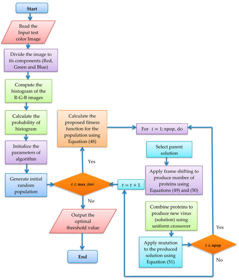
Figure 1.
Flow chart of the COVIDOA with proposed fitness function.
Computational Complexity Analysis
According to the structure of COVIDOA, it mostly involves initialization, fitness evaluation, and updating of COVIDOA solutions. Where the number of solutions is , is the dimension of the problem, and is the maximum number of iterations. The calculation is as follows: The time complexity for initialization is . Additionally, the COVIDOA calculates the fitness of each solution with a complexity of , and the computational complexity of the update of the solution vector of all solutions is . Consequently, the total computational complexity of COVIDOA is .
5. Experimental Results and Discussion
This section begins with a summary of the datasets utilized for testing. Then, we illustrate the parameter settings for the proposed and state-of-the-art algorithms, followed by the evaluation metrics utilized to compare the outcomes. The numerical outcomes of testing the proposed algorithm and its competitors are then shown. Finally, we accomplished a comparative study of the collected outcomes.
5.1. Dataset
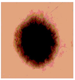
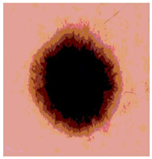
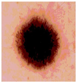
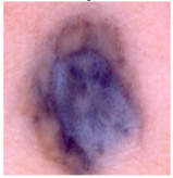
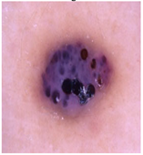
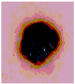
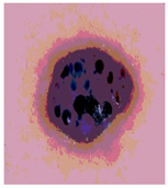
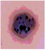
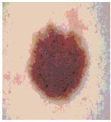
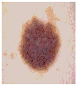
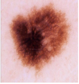
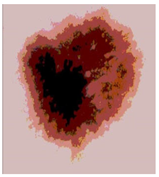
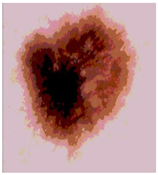
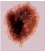
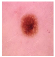
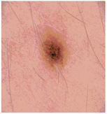
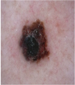
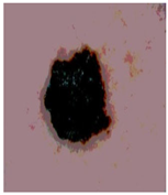
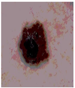
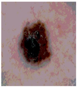
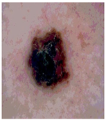
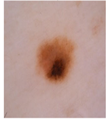
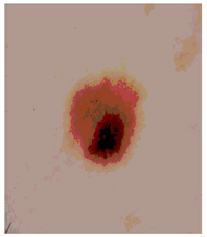
This paper uses SC images from the International Skin Imaging Collaboration (ISIC). This multinational collaboration has created the biggest public archive of dermoscopic skin images globally [70] and it is used to evaluate the proposed algorithm’s performance. More than 12,500 images across three tasks are included in this dataset.
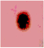
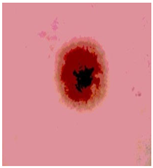
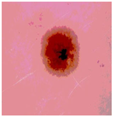
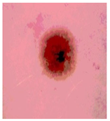
Our experiments involve segmenting 10 color images for SC using two, three, four, and five threshold levels. Those images are selected randomly from the ISIC datasets to validate the performance of COVIDOA.
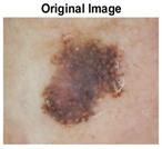
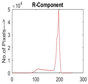
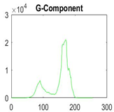
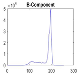
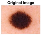
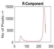
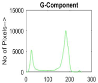
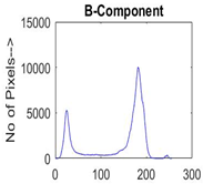
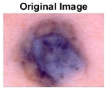
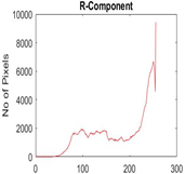
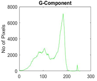
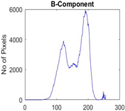
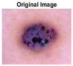
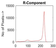
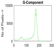
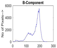
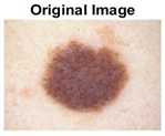
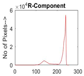
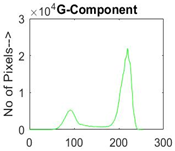
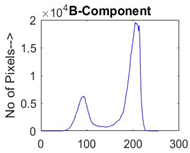
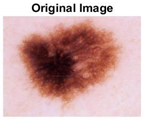
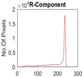
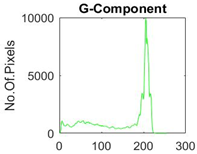
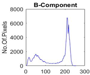
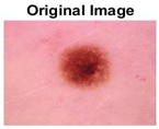
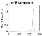
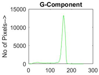
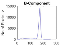
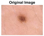
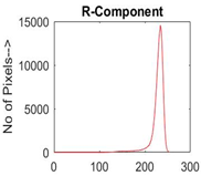
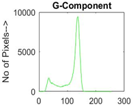
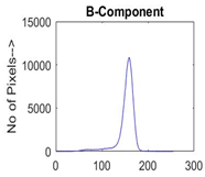
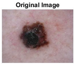
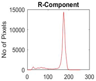
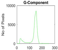
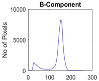
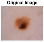
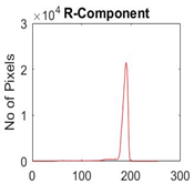
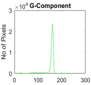
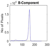
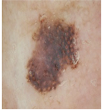
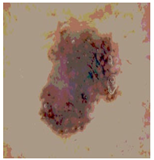
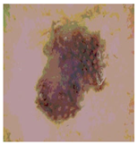
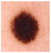
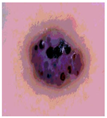
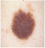
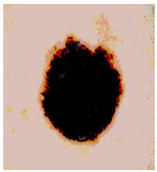
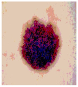
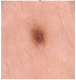
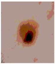
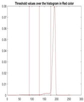
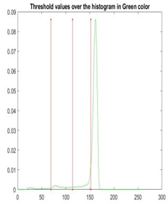
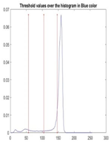
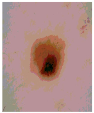
Table 1 depicts the histograms of each component and the original image, as red, green, and blue represent the three components of a color image. It is important to mention that the taken images are given new names like img1, img2, img3, img4, and so on.

Table 1.
The original SC images and their histogram of constituent colors (red, green, and blue).
5.2. Parameter Setting
The proposed algorithm’s MLT segmentation outcomes are evaluated using various criteria and compared to five popular meta-heuristic algorithms. These algorithms are AOA [71], SCA [72], RSA [73], FPA [74], SOA [75], and GTO [16].
These algorithms were chosen for comparison for the following reasons:
- They have demonstrated their superior capacity to solve several optimization challenges, particularly image segmentation.
- The majority of them are current and have been published in reliable sources.
- Their MATLAB implementations are freely accessible on the MATLAB website (https://matlab.mathworks.com/ accessed on 18 August 2023).
All experiments were conducted using a laptop equipped with an Intel (R) Core (TM) i7-1065G7 CPU, 8.0 GB of RAM, and the Windows 10 Ultimate 64-bit operating system. All of the algorithms were created with the MATLAB R2016b developing environment. As previously stated, all algorithms are tested across 30 independent runs with a population size of 50 and a maximum iteration count of 100 for each input SC test image. For all algorithms, the simulation setting is the same.
5.3. Performance Evaluation Criteria
The proposed algorithm’s performance is evaluated by four performance metrics: MSE, PSNR, FSIM, and NCC [76]. These metrics are summarized below:
5.3.1. Mean Square Error (MSE)
MSE is frequently employed to calculate the difference between the segmented and original images. It is computed in the following manner:
Here, are the intensity level of the original and segmented image within the ith row and jth column, respectively. M and N are the image’s row and column numbers, respectively.
5.3.2. Peak Signal-to-Noise Ratio (PSNR)
Another metric known as PSNR is frequently employed to quantify image quality.
It refers to the ratio of the square of the maximum gray level , and the MSE between the original and separated one is computed as follows:
MSE is computed using the equation mentioned above. Increasing PSNR is necessary to obtain higher quality.
5.3.3. Feature Similarity Index Metric (FSIM)
FSIM is utilized to compute the structural similarity of two images in the following manner:
where indicates the resemblance between the two images, is the phase congruence, and relates to the image’s spatial domain. The FSIM’s highest possible value, representing total similarity, is 1. A higher FSIM value enhances the thresholding process’s performance [77].
5.3.4. Normalized Correlation Coefficient (NCC)
NCC is a metric for determining how closely two images are connected. NCC’s absolute value varies between 0 and 1. A value of 0 shows no relationship between the two images, and 1 denotes the most powerful possible relationship. The greater the absolute value of NCC, the stronger the association between the two images. NCC between the original image and segmented images is estimated in the following manner:
5.4. Experimental Results
This subsection displays the numerical outcomes of testing the COVIDOA to choose the optimal threshold values utilizing the proposed fitness function. These outcomes are evaluated against the state-of-the-art AOA, SCA, RSA, FPA, SOA, and GTO algorithms. The experiments used two, three, four, and five threshold values. We ran the COVID optimization algorithm with classic Otsu, Kapur, and T’sallis methods, and then the outcomes of these fitness functions were compared with those of using the proposed fitness function.
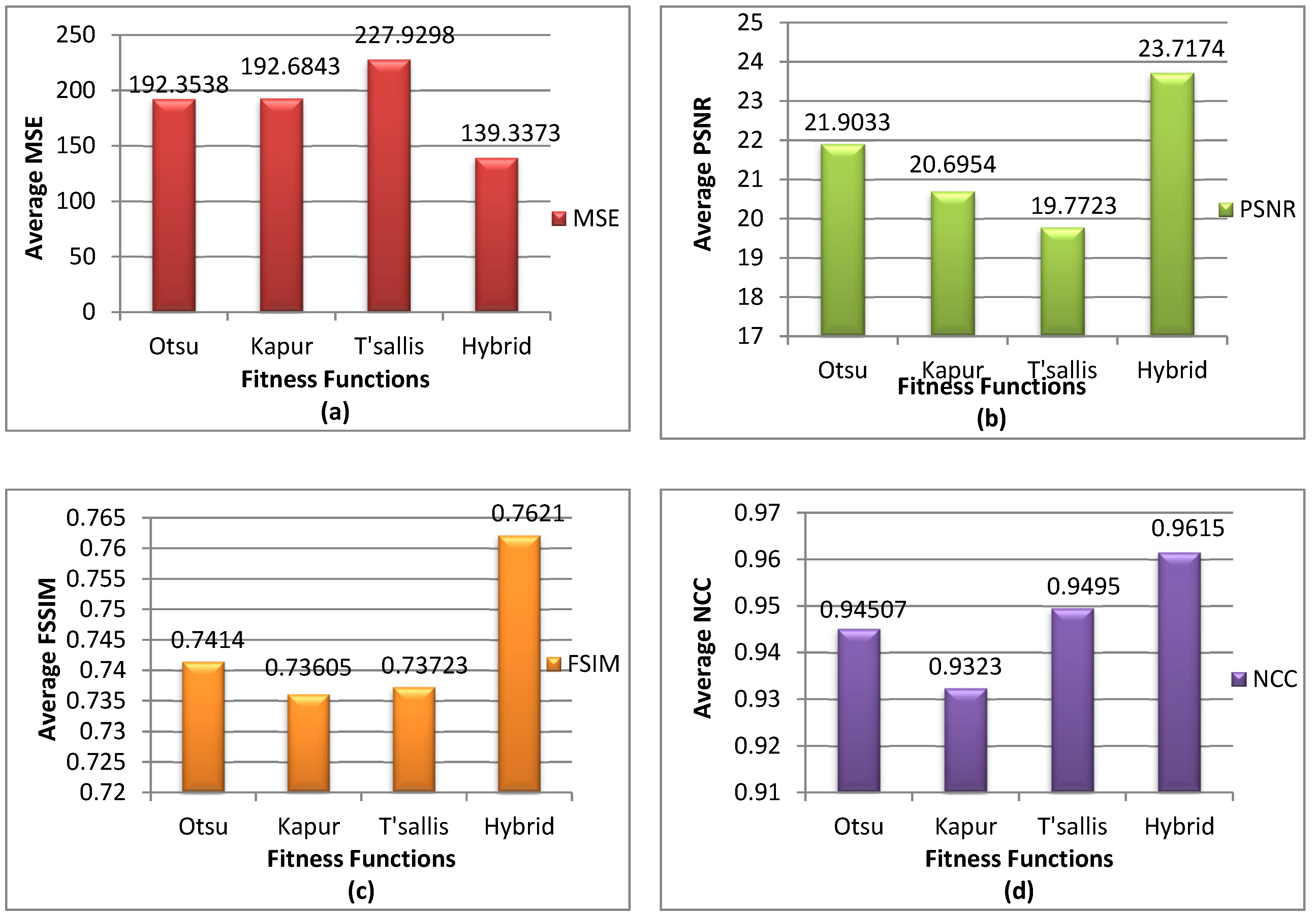
The outcomes are represented in Table 2, and Figure 2 depicts the average. From these results, we confirmed that the proposed fitness function surpasses all other fitness functions.
Table 2.
The results of the COVIDOA with all fitness functions.
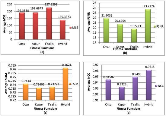
Figure 2.
The average results of (a) MSE, (b) PSNR, (c) FSIM, (d) NCC for the COVIDOA with all fitness functions.
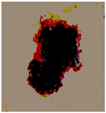
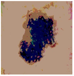
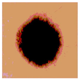
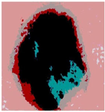
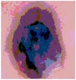
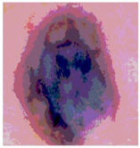
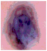
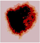
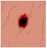
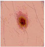
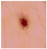
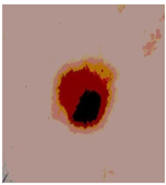
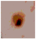
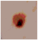
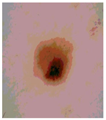
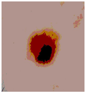
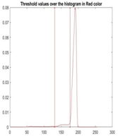
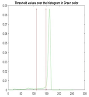
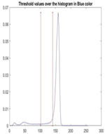
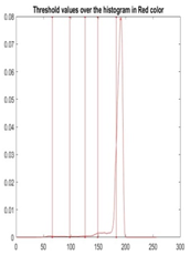
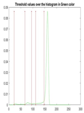
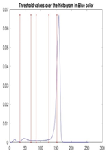
We used the proposed fitness function, as seen in Equation (48). Table 3 displays COVIDOA segmented images for all SC test images utilized in the experiments. Table 4 displays the graphs illustrating the optimal COVIDOA threshold values for RGB channels for the last test image for levels 2, 3, 4, and 5.
Table 3.
COVIDOA-acquired segmented images at Th = 2, 3, 4, and 5 with proposed fitness function.
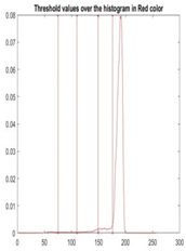
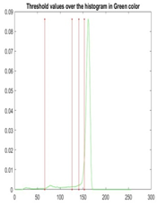
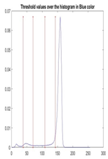
Table 4.
COVIDOA example for segmented image (image 10) and RGB channel histograms computed at Th = 2, 3, 4, and 5.
Table 5, Table 6, Table 7 and Table 8 provide the average findings of the corresponding MSE, PSNR, FSIM, and NCC evaluation matrices. The highest values of the thresholding approach, which produces the best results, are bolded in these tables. They show the optimal quality segmentation.
Table 5.
Based on the average MSE values, a comparison of COVIDOA and the other chosen algorithms.
Table 6.
Based on the mean PSNR values, the COVIDOA and the other chosen algorithms are compared.
Table 7.
Based on the mean FSIM values, a comparison of the COVIDOA and the other chosen algorithms.
Table 8.
Based on the mean NCC values, a comparison of the COVIDOA and the other chosen algorithms.
Higher mean values for PSNR, FSIM, and NCC indicate a more accurate and effective algorithm, while the lowest mean value denotes the optimum MSE value.
Table 5 lists the average values for the MSE metric. The best MSE result has the lowest mean value. It is important to note that COVIDOA surpasses all other algorithms (as previously indicated), particularly in img7 and img9, which have fewer values with all threshold levels. The SCA has lower MSE values in img1 (levels 5) and img6 (level 3), as well as the FPA in img1 (level 4), img2, and img10 (level 2).
The PSNR values are shown in Table 6 for every algorithm; a higher mean value implies superior segmentation quality. It should be noted that the COVIDOA surpasses all other algorithms in most cases.
The FSIM measure’s mean values are displayed in Table 7. This statistic examines and analyzes how well an image’s features are retained after processing. The SCA presents superior results in img1 (level 2) and img2 (level 5). Except for a few cases, the test images are not much improved by the AOA, SCA, RSA, FPA, and SOA. In comparison, the COVIDOA surpasses other algorithms in terms of FSIM on most test images.
The mean NCC values and NCC outcomes of the proposed technique (COVIDOA) outperform the other comparable algorithms, as shown in Table 8. The RSA provides a better value at only one level in img3 (level 3), GTO in img2 (levels 2 and 5), and the AOA in img2 (level 2) and img7 (level 3). The SCA gives higher results in only one image, img1 (levels 2 and 4).
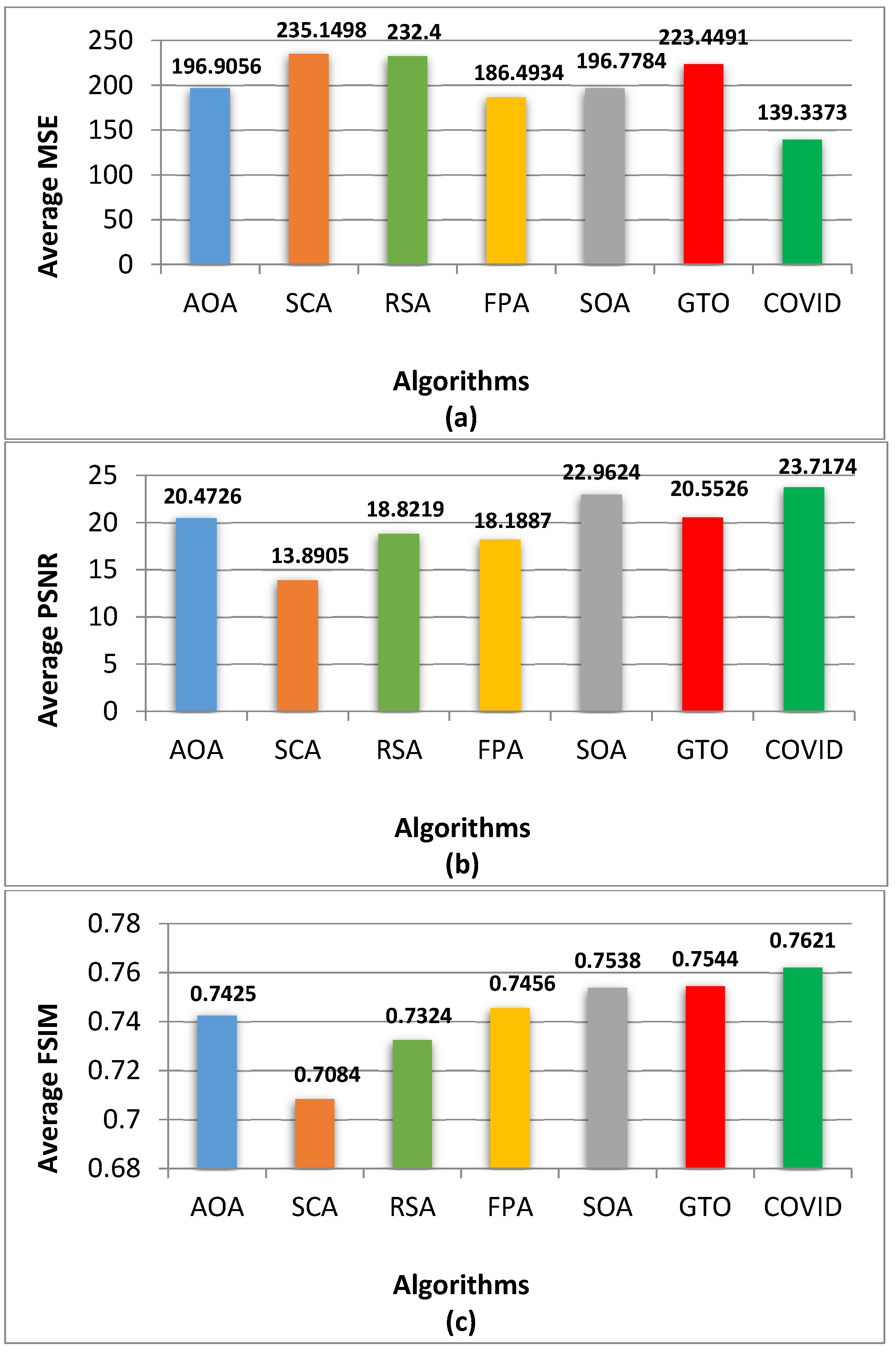
The results of comparing the COVIDOA to other algorithms are shown in Figure 3 for the overall average values for MSE, PSNR, FSIM, and NCC.

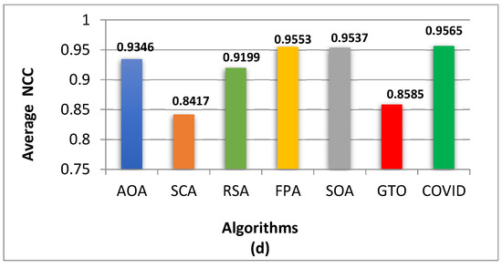
Figure 3.
The average results of (a) MSE, (b) PSNR, (c) FSIM, (d) NCC for all algorithms.
According to Figure 3, the COVIDOA has the lowest average MSE for skin lesion images. All four measures’ bar charts indicate that the COVIDOA is superior. The highest PSNR, FSIM, and NCC values produced by COVIDOA reflect the superior caliber of the segmented images.
6. Conclusions and Future Work
SC is among the most prevalent kinds of cancer; consequently, early detection can significantly lower the related mortality rate. Image segmentation is essential to any CAD system for extracting regions of interest from SC images to enhance the classification phase. One of the most successful and effective techniques for segmenting images is thresholding. This work addresses the challenge of choosing the appropriate threshold value for segmenting images in MLT. The COVIDOA with the proposed fitness function was applied to a collection of color SC images. The COVIDOA’s performance is validated using 10 skin lesion images and compared to six other meta-heuristic algorithms, AOA, SCA, RSA, FPA, SOA and GTO using a range of two to five different threshold values. The performance of the proposed algorithm has been evaluated using the following metrics: MSE, PSNR, FSIM and NCC. The outcomes of the experiments proved that the proposed fitness function improves the COVIDOA with classic Otsu, Kapur, and T’sallis fitness functions for the segmentation issue. According to the results, the COVIDOA surpasses all other algorithms regarding MSE, PSNR, FSIM, and NCC segmentation measures. The proposed method may solve various image processing difficulties and improve applications, including visualization, computer vision, CAD, and image classification. Future research should widen the examined image dataset and raise the threshold values to obtain accurate results. Furthermore, the proposed method must be evaluated with other different meta-heuristic optimization and deep learning methods to enhance the outcomes of segmentation techniques.
Future studies might involve combining the innovative COVIDOA with one of the existing meta-heuristics to address the MLT problem for skin lesion segmentation in color images. The COVIDOA developed here can solve more complex, real-world optimization problems. The proposed COVIDOA’s accuracy and resiliency may be further evaluated in various engineering and real-world situations with an unknown search space.
Author Contributions
Conceptualization, K.M.H. and D.S.E.; methodology, D.S.E., Y.S.A., and K.M.H.; software, D.S.E.; validation, Y.S.A., D.S.E., E.R.M., and K.M.H.; formal analysis, K.M.H. and E.R.M.; resources, Y.S.A., D.S.E., E.R.M., and K.M.H.; data curation, D.S.E.; writing—original draft preparation, D.S.E.; writing—review and editing, K.M.H.; visualization, D.S.E. and K.M.H.; supervision, K.M.H. All authors have read and agreed to the published version of the manuscript.
Funding
The authors declare that no funds, grants, or other support was received during the preparation of this manuscript.
Institutional Review Board Statement
Not applicable.
Informed Consent Statement
Not applicable.
Data Availability Statement
The data are available at https://www.kaggle.com/datasets/pardonndlovu/chestpelviscspinescans (accessed on 17 August 2023).
Acknowledgments
The authors would like to express their appreciation to Asmaa M. Khalid for her help and support during the completion of this research.
Conflicts of Interest
The authors declare no conflict of interest.
Abbreviations
| SC | Skin Cancer |
| UVR | Ultraviolet Radiation |
| MLT | Multilevel Thresholding |
| COVIDOA | Coronavirus Disease Optimization Algorithm |
| AOA | Arithmetic Optimization Algorithm |
| SCA | Sine Cosine Algorithm |
| RSA | Reptile Search Algorithm |
| FPA | Flower Pollination Algorithm |
| SOA | Seagull Optimization Algorithm |
| GTO | Gorilla Troops Optimizer |
| MSE | Mean Square Error |
| PSNR | Peak Signal-to-Noise Ratio |
| FSIM | Feature Similarity Index Metric |
| NCC | Normalized Correlation Coefficient |
| CAD | Computer-Aided Diagnosis |
| AI | Artificial Intelligence |
| PSO | Particle Swarm Optimization |
| WOA | Whale Optimization Algorithm |
| CSA | Cuckoo Search Algorithm |
| HHOA | Harris Hawks Optimization Algorithm |
| GWOA | Gray Wolf Optimization Algorithm |
| EOA | Equilibrium Optimization Algorithm |
| COA | Chimp Optimization Algorithm |
| MRFOA | Manta Ray Foraging Optimization Algorithm |
| SMA | Slime Mould Algorithm |
| MPA | Marine Predators Algorithm |
| BWOA | Black Widow Optimization Algorithm |
| MGWO | Multistage Grey Wolf Optimizer |
| VCS | Virus Colony Search |
| SSA | Salp Swarm Algorithm |
| FA | Firefly Algorithm |
| OBL | Opposition-Based Learning |
| ABC | Artificial Bee Colony |
| KHO | Krill Herd Optimization |
| DBN | Deep Belief Network |
| MEFOA | Modified Electromagnetic Field Optimization Algorithm |
| MAFBUZO | Multi-Agent Fuzzy Buzzard Algorithm |
| ISIC | International Skin Imaging Collaboration |
References
- Pathan, S.; Prabhu, K.G.; Siddalingaswamy, P.C. Techniques and algorithms for computer-aided diagnosis of pigmented skin lesions—A review. Biomed. Signal Process. Control 2018, 39, 237–262. [Google Scholar] [CrossRef]
- Dey, N.; Rajinikanth, V.; Ashour, A.S.; Tavares, J.M. Social group optimization supported segmentation and evaluation of skin melanoma images. Symmetry 2018, 10, 51. [Google Scholar] [CrossRef]
- Saba, T. Computer vision for microscopic skin cancer diagnosis using handcrafted and non-handcrafted features. Microsc. Res. Tech. 2021, 84, 1272–1283. [Google Scholar] [CrossRef] [PubMed]
- Pham, D.L.; Xu, C.; Prince, J.L. Current methods in medical image segmentation. Annu. Rev. Biomed. Eng. 2000, 2, 315–337. [Google Scholar] [CrossRef] [PubMed]
- Huang, Y.C.; Tung, Y.S.; Chen, J.C.; Wang, S.W.; Wu, J.L. An adaptive edge detection-based colorization algorithm and its applications. In Proceedings of the 13th Annual ACM International Conference on Multimedia, Singapore, 6–11 November 2011; pp. 351–354. [Google Scholar]
- Abonyi, J.; Feil, B.; Nemeth, S.; Arva, P. Fuzzy clustering based segmentation of time-series. In Advances in Intelligent Data Analysis V; Proceedings of the 5th International Symposium on Intelligent Data Analysis, IDA 2003; Berlin, Germany, 28–30 August 2003, Springer: Berlin/Heidelberg, Germany, 2003; pp. 275–285. [Google Scholar]
- Kohler, R. A segmentation system based on thresholding. Comput. Graph. Image Process. 1981, 15, 319–338. [Google Scholar] [CrossRef]
- Kuruvilla, J.; Sukumaran, D.; Sankar, A.; Joy, S.P. A review on image processing and image segmentation. In Proceedings of the 2016 International IEEE Conference on Data Mining and Advanced Computing (SAPIENCE), Ernakulam, India, 16–18 March 2016; pp. 198–203. [Google Scholar]
- Toma, M.; Lu, Y.; Zhou, H.; Garcia, J.D. Thresholding segmentation errors and uncertainty with patient-specific geometries. J. Biomed. Phys. Eng. 2021, 11, 115–122. [Google Scholar] [CrossRef]
- Li, W.; Raj, A.N.; Tjahjadi, T.; Zhuang, Z. Digital hair removal by deep learning for skin lesion segmentation. Pattern Recognit. 2021, 117, 107994. [Google Scholar] [CrossRef]
- Chai, Y.; Lempitsky, V.; Zisserman, A. Bicos: A bi-level co-segmentation method for image classification. In Proceedings of the 2011 International Conference on Computer Vision, Barcelona, Spain, 6–13 November 2011; pp. 2579–2586. [Google Scholar]
- Horng, M.-H. Multilevel thresholding selection based on the artificial bee colony algorithm for image segmentation. Expert Syst. Appl. 2011, 38, 13785–13791. [Google Scholar] [CrossRef]
- Otsu, N. A threshold selection method from gray-level histograms. IEEE Trans. Syst. Man Cybern. 1979, 9, 62–66. [Google Scholar] [CrossRef]
- Oliva, D.; Elaziz, M.A.; Hinojosa, S. Fuzzy entropy approaches for image segmentation. In Metaheuristic Algorithms for Image Segmentation: Theory and Applications; Springer: Cham, Switzerland, 2019; pp. 141–147. [Google Scholar]
- Kapur, J.N.; Sahoo, P.K.; Wong, A.K. A new method for gray-level picture thresholding using the entropy of the histogram. Comput. Vis. Graph. Image Process. 1985, 29, 273–285. [Google Scholar] [CrossRef]
- Abdollahzadeh, B.; Soleimanian Gharehchopogh, F.; Mirjalili, S. Artificial gorilla troops optimizer: A new nature-inspired metaheuristic algorithm for global optimization problems. Int. J. Intell. Syst. 2021, 36, 5887–5958. [Google Scholar] [CrossRef]
- Gharehchopogh, F.S.; Maleki, I.; Dizaji, Z.A. Chaotic vortex search algorithm: Meta-heuristic algorithm for feature selection. Evol. Intell. 2022, 15, 1777–1808. [Google Scholar] [CrossRef]
- Halim, Z. Optimizing the DNA fragment assembly using meta-heuristic-based overlap layout consensus approach. Appl. Soft Comput. 2020, 92, 106256. [Google Scholar]
- Meera, S.; Sundar, C. A hybrid meta-heuristic approach for efficient feature selection methods in big data. J. Ambient. Intell. Humaniz. Comput. 2021, 12, 3743–3751. [Google Scholar] [CrossRef]
- SaiSindhuTheja, R.; Shyam, G.K. An efficient meta-heuristic algorithm-based feature selection and recurrent neural network for DoS attack detection in cloud computing environment. Appl. Soft Comput. 2021, 100, 106997. [Google Scholar] [CrossRef]
- Ramadas, M.; Abraham, A. Meta-Heuristics for Data Clustering and Image Segmentation; Springer: Berlin/Heidelberg, Germany, 2019. [Google Scholar]
- Borjigin, S.; Sahoo, P.K. Color image segmentation based on multi-level Tsallis–Havrda–Charvát entropy and 2D histogram using PSO algorithms. Pattern Recognit. 2019, 92, 107–118. [Google Scholar] [CrossRef]
- Abdel-Basset, M.; Mohamed, R.; AbdelAziz, N.M.; Abouhawwash, M. HWOA: A hybrid whale optimization algorithm with a novel local minima avoidance method for multi-level thresholding color image segmentation. Expert Syst. Appl. 2022, 190, 116145. [Google Scholar] [CrossRef]
- Agrawal, S.; Panda, R.; Choudhury, P.; Abraham, A. Dominant color component and adaptive whale optimization algorithm for multilevel thresholding of color images. Knowl.-Based Syst. 2022, 240, 108172. [Google Scholar] [CrossRef]
- Eberhart, R.; Kennedy, J. Particle swarm optimization. In Proceedings of the 1995 IEEE International Conference on Neural Networks, Perth, Australia, 27 November–1 December 1995; Volume 4, pp. 1942–1948. [Google Scholar]
- Mirjalili, S.; Lewis, A. The whale optimization algorithm. Adv. Eng. Softw. 2016, 95, 51–67. [Google Scholar] [CrossRef]
- Yang, X.S.; Deb, S. Cuckoo search via Lévy flights. In Proceedings of the 2009 World Congress on Nature & Biologically Inspired Computing (NaBIC), Coimbatore, India, 9–11 December 2009; pp. 210–214. [Google Scholar]
- Heidari, A.A.; Mirjalili, S.; Faris, H.; Aljarah, I.; Mafarja, M.; Chen, H. Harris Hawks optimization: Algorithm and applications. Future Gener. Comput. Syst. 2019, 97, 849–872. [Google Scholar] [CrossRef]
- Mirjalili, S.; Mirjalili, S.M.; Lewis, A. Grey wolf optimizer. Adv. Eng. Softw. 2014, 69, 46–61. [Google Scholar] [CrossRef]
- Abdel-Basset, M.; Chang, V.; Mohamed, R. A novel equilibrium optimization algorithm for multi-thresholding image segmentation problems. Neural Comput. Appl. 2021, 33, 10685–10718. [Google Scholar] [CrossRef]
- Khishe, M.; Mosavi, M.R. Chimp optimization algorithm. Expert Syst. Appl. 2020, 149, 113338. [Google Scholar] [CrossRef]
- Zhao, W.; Zhang, Z.; Wang, L. Manta ray foraging optimization: An effective bio-inspired optimizer for engineering applications. Eng. Appl. Artif. Intell. 2020, 87, 103300. [Google Scholar] [CrossRef]
- Li, S.; Chen, H.; Wang, M.; Heidari, A.A.; Mirjalili, S. Slime mould algorithm: A new method for stochastic optimization. Future Gener. Comput. Syst. 2020, 111, 300–323. [Google Scholar] [CrossRef]
- Faramarzi, A.; Heidarinejad, M.; Mirjalili, S.; Gandomi, A.H. Marine Predators Algorithm: A nature-inspired meta-heuristic. Expert Syst. Appl. 2020, 152, 113377. [Google Scholar] [CrossRef]
- Hayyolalam, V.; Kazem, A.A.P. Black widow optimization algorithm: A novel meta-heuristic approach for solving engineering optimization problems. Eng. Appl. Artif. Intell. 2020, 87, 103249. [Google Scholar] [CrossRef]
- Khalid, A.M.; Hosny, K.M.; Mirjalili, S. COVIDOA: A novel evolutionary optimization algorithm based on coronavirus disease replication lifecycle. Neural Comput. Appl. 2022, 34, 22465–22492. [Google Scholar] [CrossRef]
- Rai, R.; Das, A.; Dhal, K.G. Nature-inspired optimization algorithms and their significance in multi-thresholding image segmentation: An inclusive review. Evol. Syst. 2022, 13, 889–945. [Google Scholar] [CrossRef]
- Sharma, A.; Chaturvedi, R.; Bhargava, A. A novel opposition-based improved firefly algorithm for multilevel image segmentation. Multimed. Tools Appl. 2022, 81, 15521–15544. [Google Scholar] [CrossRef]
- Yu, H.; Song, J.; Chen, C.; Heidari, A.A.; Liu, J.; Chen, H.; Zaguia, A.; Mafarja, M. Image segmentation of Leaf Spot Diseases on Maize using multi-stage Cauchy-enabled grey wolf algorithm. Eng. Appl. Artif. Intell. 2022, 109, 104653. [Google Scholar] [CrossRef]
- Hussien, A.G.; Heidari, A.A.; Ye, X.; Liang, G.; Chen, H.; Pan, Z. Boosting whale optimization with evolution strategy and Gaussian random walks: An image segmentation method. Eng. Comput. 2023, 39, 1935–1979. [Google Scholar] [CrossRef]
- Yu, M.; Han, M.; Li, X.; Wei, X.; Jiang, H.; Chen, H.; Yu, R. Adaptive soft erasure with edge self-attention for weakly supervised semantic segmentation: Thyroid ultrasound image case study. Comput. Biol. Med. 2022, 144, 105347. [Google Scholar] [CrossRef]
- Qi, A.; Zhao, D.; Yu, F.; Heidari, A.A.; Wu, Z.; Cai, Z.; Alenezi, F.; Mansour, R.F.; Chen, H.; Chen, M. Directional mutation and crossover boosted ant colony optimization with application to COVID-19 X-ray image segmentation. Comput. Biol. Med. 2022, 148, 105810. [Google Scholar] [CrossRef]
- Vijh, S.; Saraswat, M.; Kumar, S. Automatic multilevel image thresholding segmentation using hybrid bio-inspired algorithm and artificial neural network for histopathology images. Multimed. Tools Appl. 2023, 82, 4979–5010. [Google Scholar] [CrossRef]
- Bhavani, H.R.; Champa, H.N. A multilevel thresholding method based on HPSO for the segmentation of various objective functions. In Proceedings of the 2022 International Conference on Communication, Computing, and Internet of Things (IC3IoT), Chennai, India, 10–11 March 2022; pp. 1–5. [Google Scholar]
- Choudhury, A.; Samanta, S.; Pratihar, S.; Bandyopadhyay, O. Multilevel segmentation of Hippocampus images using global steered quantum inspired firefly algorithm. Appl. Intell. 2022, 52, 7339–7372. [Google Scholar] [CrossRef]
- Dinkar, S.K.; Deep, K.; Mirjalili, S.; Thapliyal, S. Opposition-based Laplacian equilibrium optimizer with application in image segmentation using multilevel thresholding. Expert Syst. Appl. 2021, 174, 114766. [Google Scholar] [CrossRef]
- Zhou, Y.; Yang, X.; Ling, Y.; Zhang, J. Meta-heuristic moth swarm algorithm for multilevel thresholding image segmentation. Multimed. Tools Appl. 2018, 77, 23699–23727. [Google Scholar] [CrossRef]
- Zhang, S.; Jiang, W.; Satoh, S.I. Multilevel thresholding color image segmentation using a modified artificial bee colony algorithm. IEICE Trans. Inf. Syst. 2018, 101, 2064–2071. [Google Scholar] [CrossRef]
- Chakraborty, F.; Roy, P.K.; Nandi, D. Oppositional elephant herding optimization with dynamic Cauchy mutation for multilevel image thresholding. Evol. Intell. 2019, 12, 445–467. [Google Scholar] [CrossRef]
- Yan, Z.; Zhang, J.; Yang, Z.; Tang, J. Kapur’s entropy for underwater multilevel thresholding image segmentation based on whale optimization algorithm. IEEE Access 2020, 9, 41294–41319. [Google Scholar] [CrossRef]
- Resma, K.B.; Nair, M.S. Multilevel thresholding for image segmentation using Krill Herd Optimization algorithm. J. King Saud Univ.-Comput. Inf. Sci. 2021, 33, 528–541. [Google Scholar]
- Chakraborty, S.; Mali, K.; Banerjee, A.; Bhattacharjee, M.; Chatterjee, S. Image segmentation based on galactic swarm optimization. In Advances in Smart Communication Technology and Information Processing: OPTRONIX 2020; Springer: Singapore, 2021; pp. 251–258. [Google Scholar]
- Anitha, J.; Pandian, S.I.A.; Agnes, S.A. An efficient multilevel color image thresholding based on modified whale optimization algorithm. Expert Syst. Appl. 2021, 178, 115003. [Google Scholar] [CrossRef]
- Abualigah, L.; Habash, M.; Hanandeh, E.S.; Hussein, A.M.; Al Shinwan, M.; Abu Zitar, R.; Jia, H. Improved Reptile Search algorithm by Salp Swarm algorithm for medical image segmentation. J. Bionic Eng. 2023, 20, 1766–1790. [Google Scholar] [CrossRef] [PubMed]
- Hao, S.; Huang, C.; Heidari, A.A.; Chen, H.; Li, L.; Algarni, A.D.; Elmannai, H.; Xu, S. Salp swarm algorithm with iterative mapping and local escaping for multi-level threshold image segmentation: A skin cancer dermoscopic case study. J. Comput. Des. Eng. 2023, 10, 655–693. [Google Scholar] [CrossRef]
- Huang, Q.; Ding, H.; Sheykhahmad, F.R. A skin cancer diagnosis system for dermoscopy images according to deep training and metaheuristics. Biomed. Signal Process. Control 2023, 83, 104705. [Google Scholar] [CrossRef]
- Emam, M.M.; Houssein, E.H.; Ghoniem, R.M. A modified reptile search algorithm for global optimization and image segmentation: Case study brain MRI images. Comput. Biol. Med. 2023, 152, 106404. [Google Scholar] [CrossRef] [PubMed]
- Razmjooy, N.; Arshaghi, A. Application of Multilevel Thresholding and CNN for the Diagnosis of Skin Cancer Utilizing a Multi-Agent Fuzzy Buzzard Algorithm. Biomed. Signal Process. Control 2023, 84, 104984. [Google Scholar] [CrossRef]
- Hosny, K.M.; Khalid, A.M.; Hamza, H.M.; Mirjalili, S. Multilevel segmentation of 2D and volumetric medical images using hybrid Coronavirus Optimization Algorithm. Comput. Biol. Med. 2022, 150, 106003. [Google Scholar] [CrossRef] [PubMed]
- Hosny, K.M.; Khalid, A.M.; Hamza, H.M.; Mirjalili, S. Multilevel thresholding satellite image segmentation using chaotic coronavirus optimization algorithm with hybrid fitness function. Neural Comput. Appl. 2022, 35, 855–886. [Google Scholar] [CrossRef] [PubMed]
- Sezgin, M.; Sankur, B.L. Survey over image thresholding techniques and quantitative performance evaluation. J. Electron. Imaging 2004, 13, 146–168. [Google Scholar]
- Pare, S.; Kumar, A.; Bajaj, V.; Singh, G.K. A multilevel color image segmentation technique based on cuckoo search algorithm and energy curve. Appl. Soft Comput. 2016, 47, 76–102. [Google Scholar] [CrossRef]
- Pare, S.; Kumar, A.; Bajaj, V.; Singh, G.K. An efficient method for multilevel color image thresholding using cuckoo search algorithm based on minimum cross entropy. Appl. Soft Comput. 2017, 61, 570–592. [Google Scholar] [CrossRef]
- Agrawal, S.; Panda, R.; Bhuyan, S.; Panigrahi, B.K. Tsallis entropy-based optimal multilevel thresholding using cuckoo search algorithm. Swarm Evol. Comput. 2013, 11, 16–30. [Google Scholar] [CrossRef]
- Khalid, A.M.; Hamza, H.M.; Mirjalili, S.; Hosny, K.M. BCOVIDOA: A novel binary coronavirus disease optimization algorithm for feature selection. Knowl.-Based Syst. 2022, 248, 108789. [Google Scholar] [CrossRef] [PubMed]
- Ahn, D.-G.; Lee, W.; Choi, J.-K.; Kim, S.-J.; Plant, E.P.; Almazán, F.; Taylor, D.R.; Enjuanes, L.; Oh, J.-W. Interference of ribosomal frameshifting by antisense peptide nucleic acids suppresses SARS coronavirus replication. Antivir. Res. 2011, 91, 1–10. [Google Scholar] [CrossRef]
- Kelly, J.A.; Olson, A.N.; Neupane, K.; Munshi, S.; San Emeterio, J.; Pollack, L.; Woodside, M.T.; Dinman, J.D. Structural and functional conservation of the programmed− 1 ribosomal frameshift signal of SARS coronavirus 2 (SARS-CoV-2). J. Biol. Chem. 2020, 295, 10741–10748. [Google Scholar] [CrossRef] [PubMed]
- Brian, D.A.; Baric, R.S. Coronavirus genome structure and replication. In Coronavirus Replication and Reverse Genetics; Springer: Berlin/Heidelberg, Germany, 2005; pp. 1–30. [Google Scholar]
- Khan, M.I.; Khan, Z.A.; Baig, M.H.; Ahmad, I.; Farouk, A.E.; Song, Y.G.; Dong, J.-J. Comparative genome analysis of novel coronavirus (SARS-CoV-2) from different geographical locations and the effect of mutations on major target proteins: An in silico insight. PLoS ONE 2020, 15, e0238344. [Google Scholar] [CrossRef] [PubMed]
- Codella, N.; Rotemberg, V.; Tschandl, P.; Celebi, M.E.; Dusza, S.; Gutman, D.; Helba, B.; Kalloo, A.; Liopyris, K.; Marchetti, M.; et al. Skin lesion analysis toward melanoma detection 2018: A challenge hosted by the international skin imaging collaboration (ISIC). arXiv 2019, arXiv:1902.03368. [Google Scholar]
- Abualigah, L.; Diabat, A.; Mirjalili, S.; Abd Elaziz, M.; Gandomi, A.H. The arithmetic optimization algorithm. Comput. Methods Appl. Mech. Eng. 2021, 376, 113609. [Google Scholar] [CrossRef]
- Mirjalili, S. SCA: A sine cosine algorithm for solving optimization problems. Knowl.-Based Syst. 2016, 96, 120–133. [Google Scholar] [CrossRef]
- Abualigah, L.; Abd Elaziz, M.; Sumari, P.; Geem, Z.W.; Gandomi, A.H. Reptile Search Algorithm (RSA): A nature-inspired meta-heuristic optimizer. Expert Syst. Appl. 2022, 191, 116158. [Google Scholar] [CrossRef]
- Shen, L.; Fan, C.; Huang, X. Multi-level image thresholding using modified flower pollination algorithm. IEEE Access 2018, 6, 30508–30519. [Google Scholar] [CrossRef]
- Wang, Y. Otsu image threshold segmentation method based on seagull optimization algorithm. J. Phys. Conf. Ser. 2020, 1650, 032181. [Google Scholar] [CrossRef]
- Sara, U.; Akter, M.; Uddin, M.S. Image quality assessment through FSIM, SSIM, MSE, and PSNR—A comparative study. J. Comput. Commun. 2019, 7, 8–18. [Google Scholar] [CrossRef]
- Zhang, L.; Zhang, L.; Mou, X.; Zhang, D. FSIM: A feature similarity index for image quality assessment. IEEE Trans. Image Process. 2011, 20, 2378–2386. [Google Scholar] [CrossRef] [PubMed]


Disclaimer/Publisher’s Note: The statements, opinions and data contained in all publications are solely those of the individual author(s) and contributor(s) and not of MDPI and/or the editor(s). MDPI and/or the editor(s) disclaim responsibility for any injury to people or property resulting from any ideas, methods, instructions or products referred to in the content. |
© 2023 by the authors. Licensee MDPI, Basel, Switzerland. This article is an open access article distributed under the terms and conditions of the Creative Commons Attribution (CC BY) license (https://creativecommons.org/licenses/by/4.0/).