

Image Embeddings Extracted from CNNs Outperform Other Transfer Learning Approaches in Classification of Chest Radiographs

 , ,
, ,  , ,
, ,
Abstract
:1. Introduction
- Identification of the best transfer learning approach for medical imaging classification, encompassing three steps: (1) pretraining of CNN models on a large publicly available dataset, (2) development of multiple transfer learning methods, and (3) performance evaluation and comparison;
- Interpretation of CNN black-box predictions using explainable AI (XAI) on a population level and randomly selected set of examples.
2. Materials and Methods
2.1. Datasets
2.2. Pretraining on CheXpert
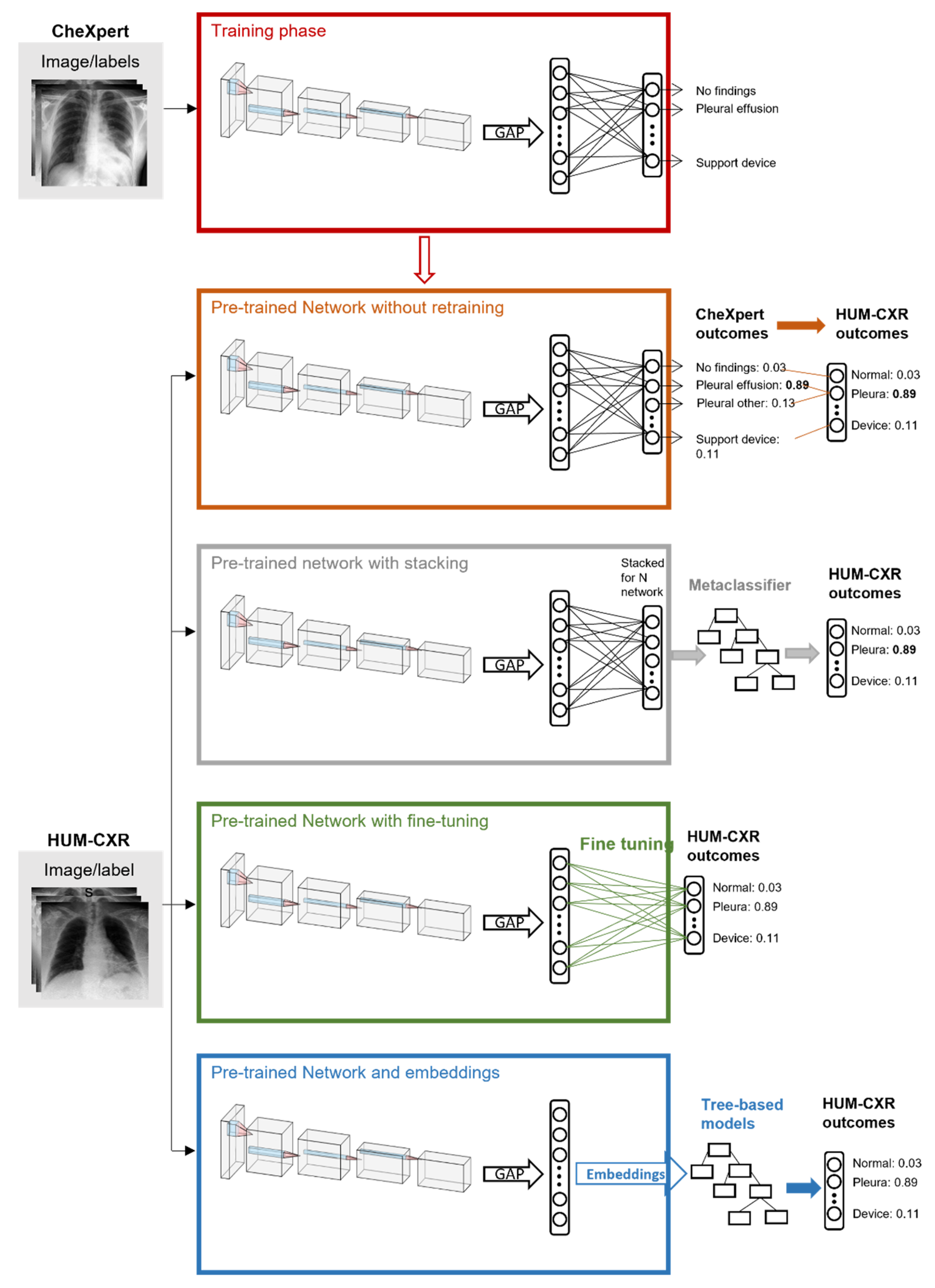
2.3. Transfer Learning
2.4. Performance Assessment
2.5. Explainability
3. Results
3.1. Baseline with Pretrained CNN
3.2. Stacking and Embeddings
3.3. Fine Tuning
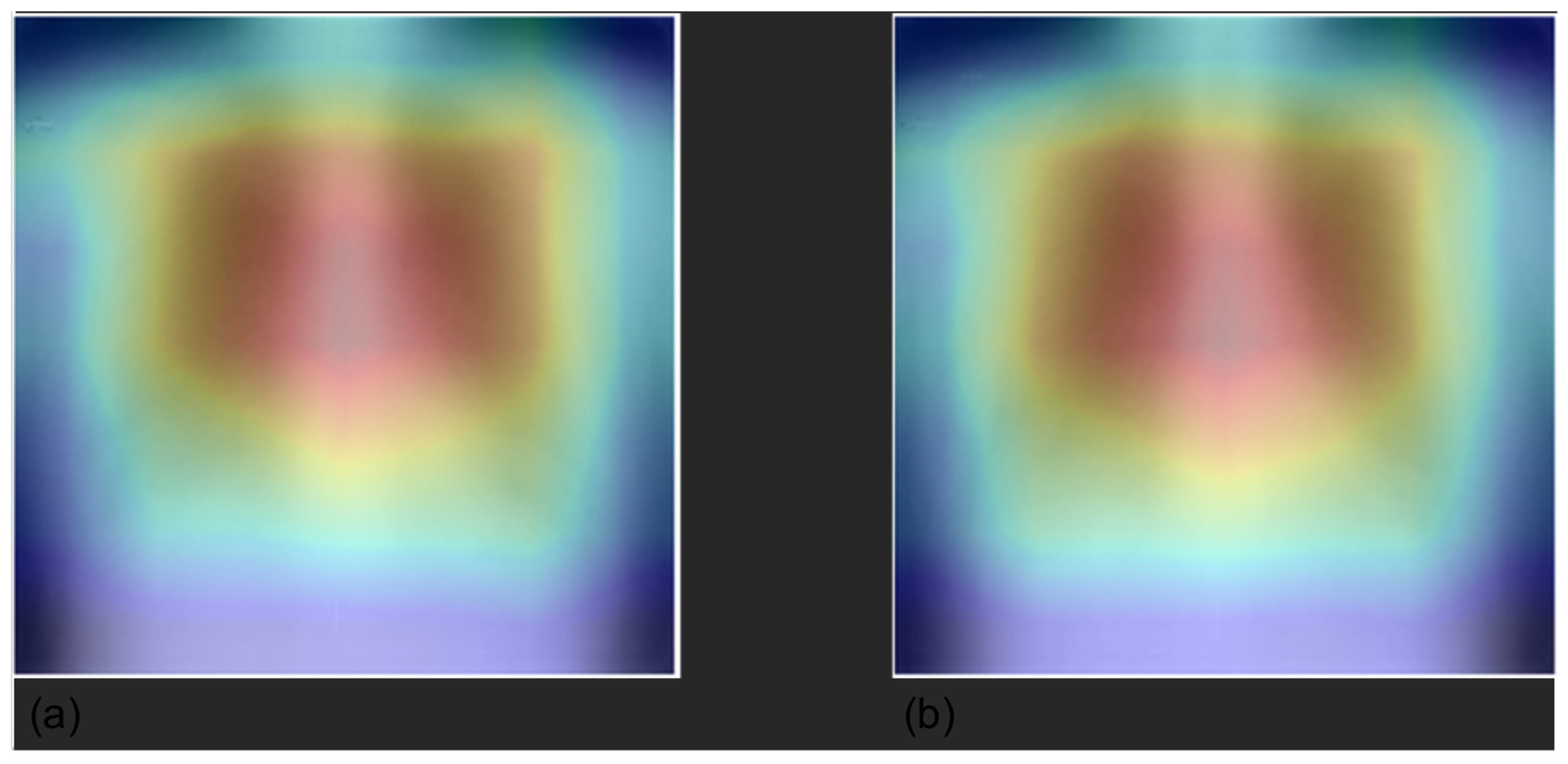
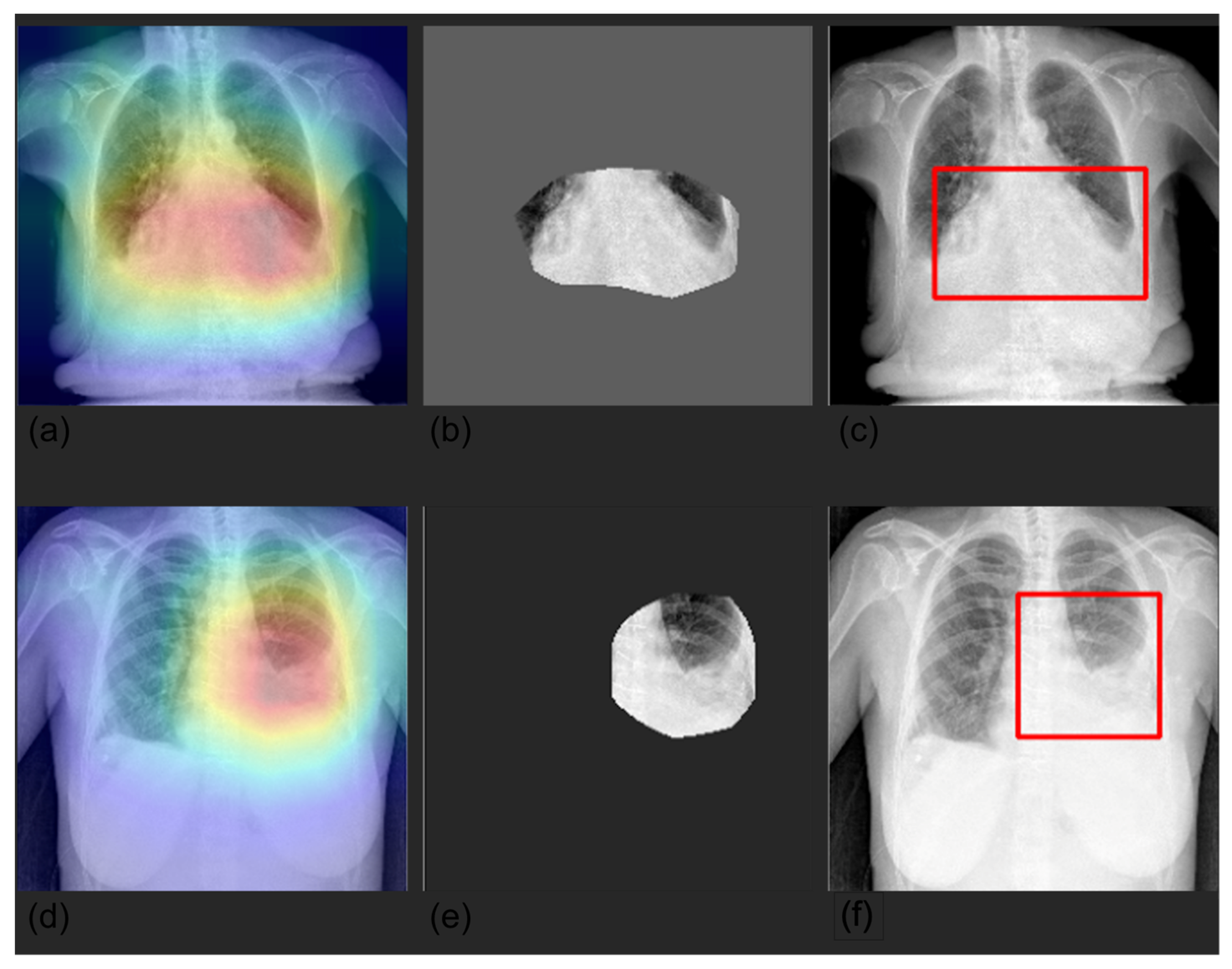
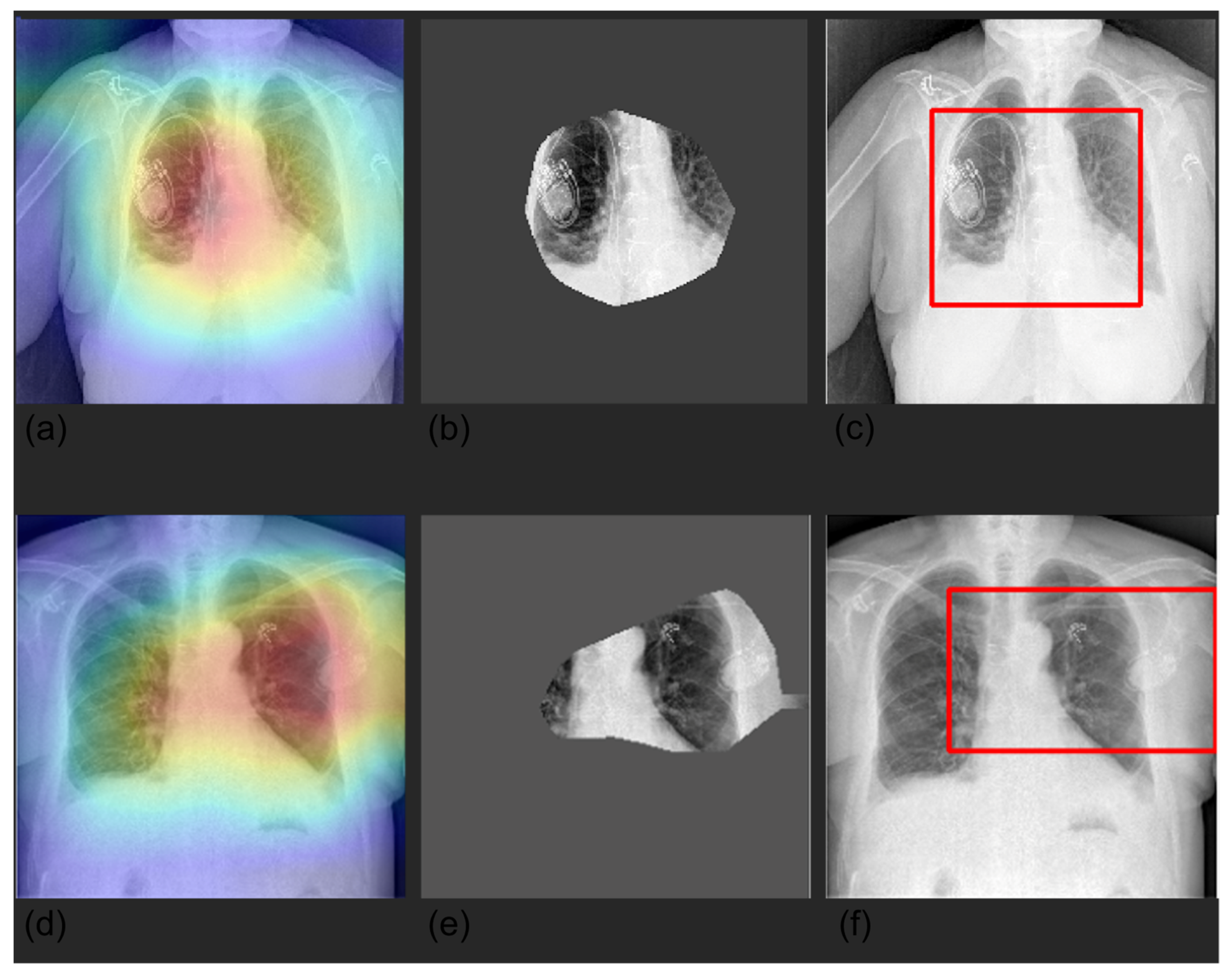
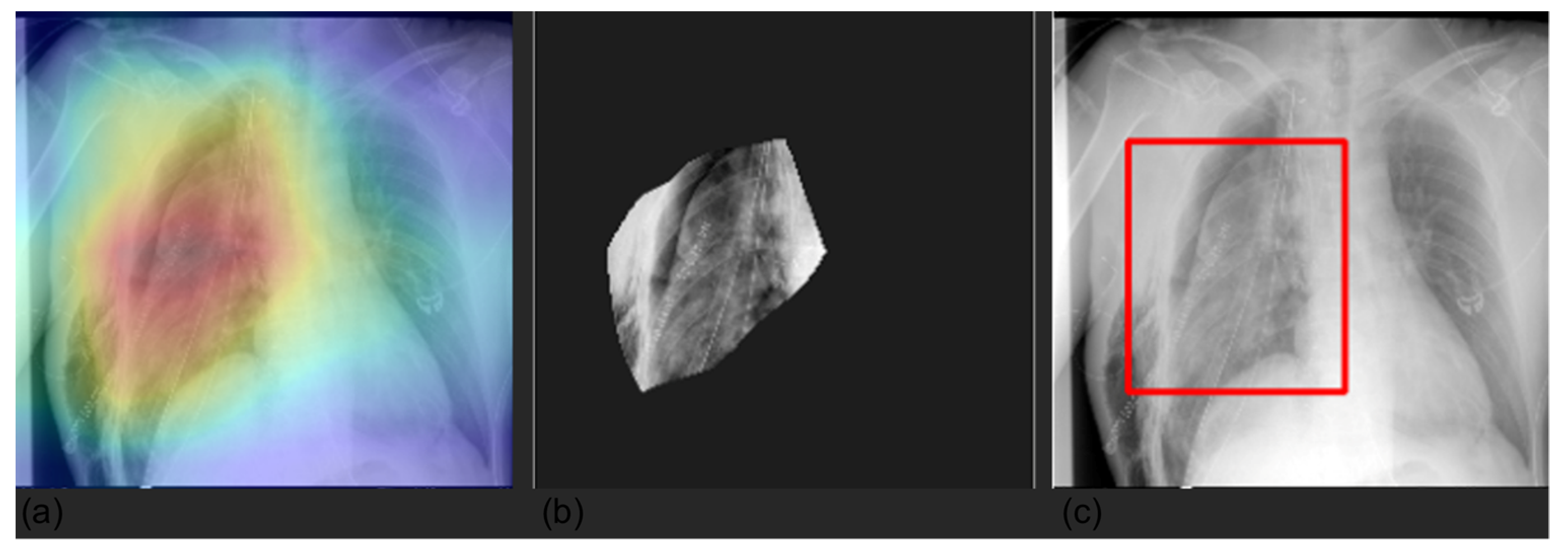
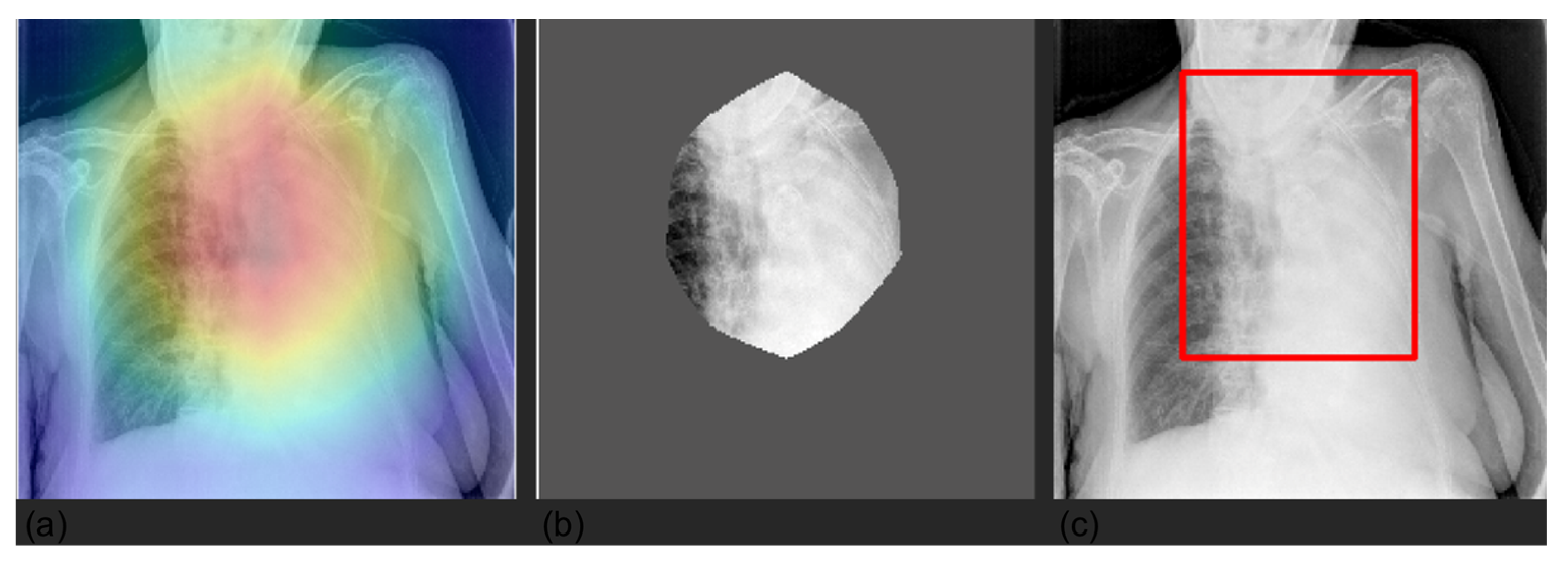
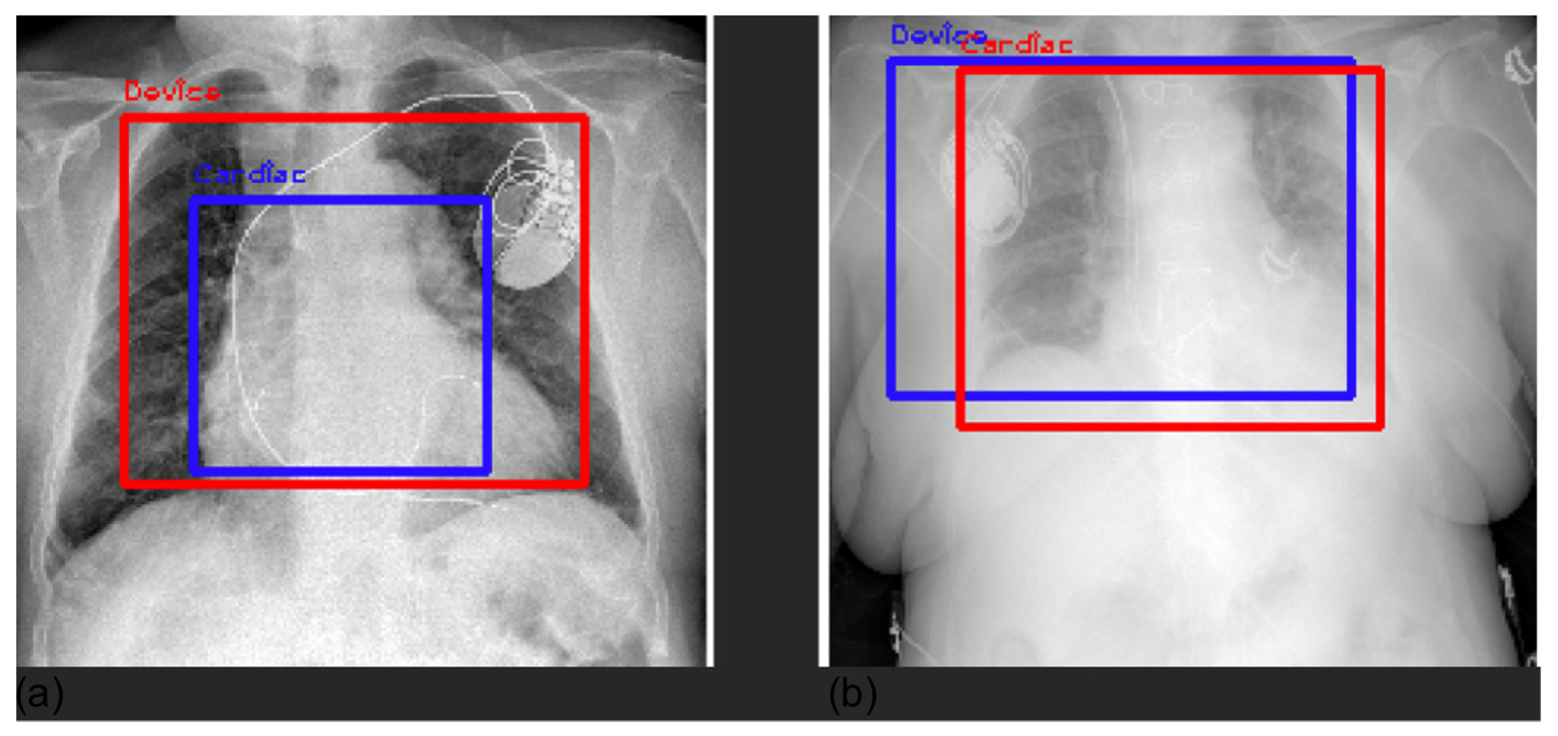
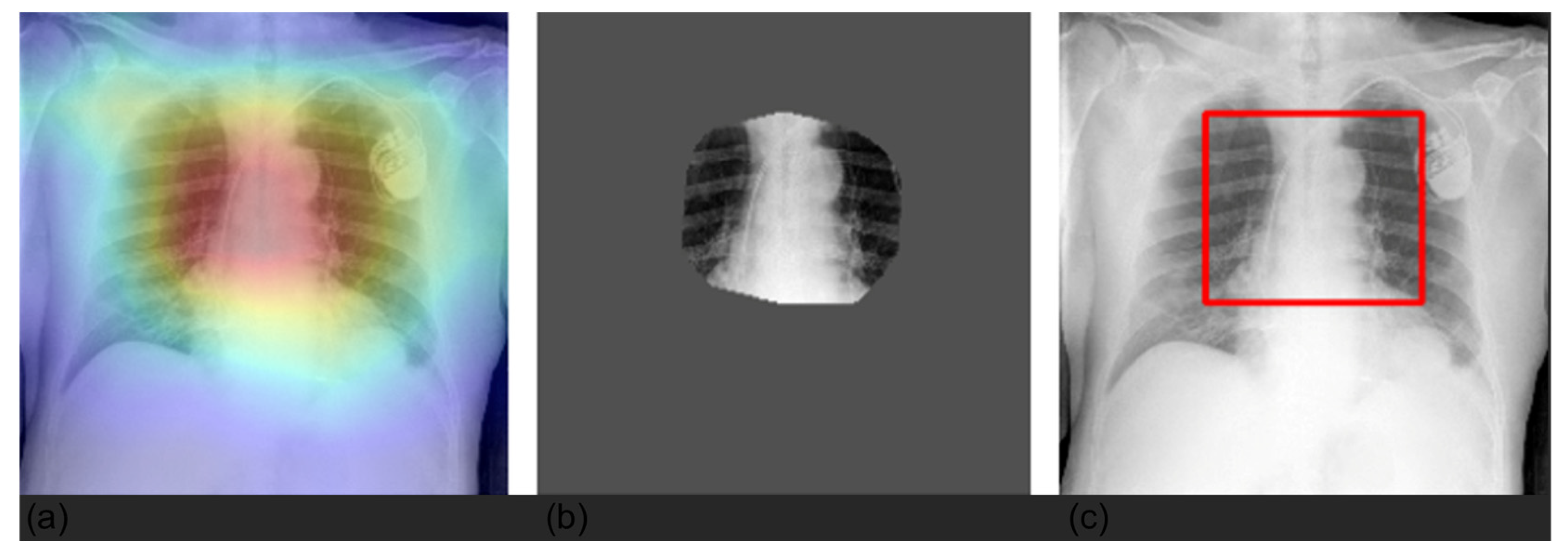
3.4. Grad-CAM
4. Discussion
5. Conclusions
Author Contributions
Funding
Institutional Review Board Statement
Informed Consent Statement
Data Availability Statement
Acknowledgments
Conflicts of Interest
References
- Kelly, C.J.; Karthikesalingam, A.; Suleyman, M.; Corrado, G.; King, D. Key challenges for delivering clinical impact with artificial intelligence. BMC Med. 2019, 17, 195. [Google Scholar] [CrossRef]
- Sollini, M.; Bartoli, F.; Marciano, A.; Zanca, R.; Slart, R.H.J.A.; Erba, P.A. Artificial intelligence and hybrid imaging: The best match for personalized medicine in oncology. Eur. J. Hybrid Imaging 2020, 4, 24. [Google Scholar] [CrossRef]
- Benjamens, S.; Dhunnoo, P.; Meskó, B. The state of artificial intelligence-based FDA-approved medical devices and algorithms: An online database. NPJ Digit. Med. 2020, 3, 118. [Google Scholar] [CrossRef]
- McKinney, S.M.; Sieniek, M.; Godbole, V.; Godwin, J.; Antropova, N.; Ashrafian, H.; Back, T.; Chesus, M.; Corrado, G.S.; Darzi, A.; et al. International evaluation of an AI system for breast cancer screening. Nature 2020, 577, 89–94. [Google Scholar] [CrossRef]
- Haenssle, H.A.; Fink, C.; Schneiderbauer, R.; Toberer, F.; Buhl, T.; Blum, A.; Kalloo, A.; Hassen, A.B.H.; Thomas, L.; Enk, A.; et al. Man against machine: Diagnostic performance of a deep learning convolutional neural network for dermoscopic melanoma recognition in comparison to 58 dermatologists. Ann. Oncol. 2018, 29, 1836–1842. [Google Scholar] [CrossRef]
- Porenta, G. Is there value for artificial intelligence applications in molecular imaging and nuclear medicine? J. Nucl. Med. 2019, 60, 1347–1349. [Google Scholar] [CrossRef]
- Sollini, M.; Antunovic, L.; Chiti, A.; Kirienko, M. Towards clinical application of image mining: A systematic review on artificial intelligence and radiomics. Eur. J. Nucl. Med. Mol. Imaging 2019, 46, 2656–2672. [Google Scholar] [CrossRef]
- Aggarwal, R.; Sounderajah, V.; Martin, G.; Ting, D.S.W.; Karthikesalingam, A.; King, D.; Ashrafian, H.; Darzi, A. Diagnostic accuracy of deep learning in medical imaging: A systematic review and meta-analysis. NPJ Digit. Med. 2021, 4, 65. [Google Scholar] [CrossRef]
- Gelardi, F.; Kirienko, M.; Sollini, M. Climbing the steps of the evidence-based medicine pyramid: Highlights from Annals of Nuclear Medicine 2019. Eur. J. Nucl. Med. Mol. Imaging 2021, 48, 1293–1301. [Google Scholar] [CrossRef]
- Abadi, E.; Segars, W.P.; Tsui, B.M.W.; Kinahan, P.E.; Bottenus, N.; Frangi, A.F.; Maidment, A.; Lo, J.; Samei, E. Virtual clinical trials in medical imaging: A review. J. Med. Imaging 2020, 7, 042805. [Google Scholar] [CrossRef] [Green Version]
- Kirienko, M.; Sollini, M.; Ninatti, G.; Loiacono, D.; Giacomello, E.; Gozzi, N.; Amigoni, F.; Mainardi, L.; Lanzi, P.L.; Chiti, A. Distributed learning: A reliable privacy-preserving strategy to change multicenter collaborations using AI. Eur. J. Nucl. Med. Mol. Imaging 2021, 48, 3791–3804. [Google Scholar] [CrossRef]
- Tajbakhsh, N.; Shin, J.Y.; Gurudu, S.R.; Hurst, R.T.; Kendall, C.B.; Gotway, M.B.; Liang, J. Convolutional neural networks for medical image analysis: Full training or fine tuning? IEEE Trans. Med. Imaging 2016, 35, 1299–1312. [Google Scholar] [CrossRef]
- Yosinski, J.; Clune, J.; Bengio, Y.; Lipson, H. How transferable are features in deep neural networks? In Proceedings of the 27th International Conference on Neural Information Processing Systems, Montreal, QC, Canada, 8–13 December 2014; MIT Press: Cambridge, MA, USA, 2014; Volume 2, pp. 3320–3328. [Google Scholar]
- Irvin, J.; Rajpurkar, P.; Ko, M.; Yu, Y.; Ciurea-Ilcus, S.; Chute, C.; Marklund, H.; Haghgoo, B.; Ball, R.; Shpanskaya, K.; et al. CheXpert: A large chest radiograph dataset with uncertainty labels and expert comparison. Proc. AAAI Conf. Artif. Intell. 2019, 33, 590–597. [Google Scholar] [CrossRef]
- Giacomello, E.; Lanzi, P.L.; Loiacono, D.; Nassano, L. Image embedding and model ensembling for automated chest X-ray interpretation. In Proceedings of the 2021 International Joint Conference on Neural Networks (IJCNN), Shenzhen, China, 18–22 July 2021. [Google Scholar]
- Huang, G.; Liu, Z.; Van Der Maaten, L.; Weinberger, K.Q. Densely connected convolutional networks. In Proceedings of the 2017 IEEE Conference on Computer Vision and Pattern Recognition (CVPR), Honolulu, HI, USA, 21–26 July 2017; IEEE: Manhattan, NY, USA, 2017. [Google Scholar]
- Szegedy, C.; Ioffe, S.; Vanhoucke, V.; Alemi, A.A. Inception-v4, inception-ResNet and the impact of residual connections on learning. In Proceedings of the Thirty-First AAAI Conference on Artificial Intelligence, San Francisco, CA, USA, 4–9 February 2017; AAAI Press: Palo Alto, CA, USA, 2017; pp. 4278–4284. [Google Scholar]
- Chollet, F. Xception: Deep learning with depthwise separable convolutions. In Proceedings of the 2017 IEEE Conference on Computer Vision and Pattern Recognition (CVPR), Honolulu, HI, USA, 21–26 July 2017; IEEE: Manhattan, NY, USA, 2017. [Google Scholar]
- Simonyan, K.; Zisserman, A. Very deep convolutional networks for large-scale image recognition. In Proceedings of the 3rd International Conference on Learning Representations, ICLR 2015, San Diego, CA, USA, 7–9 May 2015; Conference Track Proceedings. Bengio, Y., LeCun, Y., Eds.; 2015. [Google Scholar]
- Lin, M.; Chen, Q.; Yan, S. Network in network. arXiv 2013, arXiv:1312.4400. [Google Scholar]
- Deng, J.; Dong, W.; Socher, R.; Li, L.-J.; Li, K.; Fei-Fei, L. ImageNet: A large-scale hierarchical image database. In Proceedings of the 2009 IEEE Conference on Computer Vision and Pattern Recognition, Miami, FL, USA, 20–25 June 2009; IEEE: Manhattan, NY, USA, 2009. [Google Scholar]
- Wolpert, D.H. Stacked generalization. Neural Netw. 1992, 5, 241–259. [Google Scholar] [CrossRef]
- Pham, H.H.; Le, T.T.; Tran, D.Q.; Ngo, D.T.; Nguyen, H.Q. Interpreting chest X-rays via CNNs that exploit disease dependencies and uncertainty labels. medRxiv 2019. [Google Scholar] [CrossRef]
- Mandrekar, J.N. Receiver operating characteristic curve in diagnostic test assessment. J. Thorac. Oncol. 2010, 5, 1315–1316. [Google Scholar] [CrossRef]
- Barredo Arrieta, A.; Díaz-Rodríguez, N.; Del Ser, J.; Bennetot, A.; Tabik, S.; Barbado, A.; Garcia, S.; Gil-Lopez, S.; Molina, D.; Benjamins, R.; et al. Explainable Artificial Intelligence (XAI): Concepts, taxonomies, opportunities and challenges toward responsible AI. Inf. Fus. 2020, 58, 82–115. [Google Scholar] [CrossRef]
- Selvaraju, R.R.; Cogswell, M.; Das, A.; Vedantam, R.; Parikh, D.; Batra, D. Grad-CAM: Visual explanations from deep networks via gradient-based localization. In Proceedings of the 2017 IEEE International Conference on Computer Vision (ICCV), Venice, Italy, 22–29 October 2017; IEEE: Manhattan, NY, USA, 2017. [Google Scholar]
- DeGrave, A.J.; Janizek, J.D.; Lee, S.-I. AI for radiographic COVID-19 detection selects shortcuts over signal. Nat. Mach. Intell. 2021, 3, 610–619. [Google Scholar] [CrossRef]
- LeCun, Y.; Boser, B.; Denker, J.S.; Henderson, D.; Howard, R.E.; Hubbard, W.; Jackel, L.D. Backpropagation applied to handwritten zip code recognition. Neural Comput. 1989, 1, 541–551. [Google Scholar] [CrossRef]
- Cui, Y.; Song, Y.; Sun, C.; Howard, A.; Belongie, S. Large scale fine-grained categorization and domain-specific transfer learning. In Proceedings of the IEEE Conference on Computer Vision and Pattern Recognition, Salt Lake City, UT, USA, 18–23 June 2018; pp. 4109–4118. [Google Scholar]
- Ge, W.; Yu, Y. Borrowing treasures from the wealthy: Deep transfer learning through selective joint fine-tuning. In Proceedings of the 2017 IEEE Conference on Computer Vision and Pattern Recognition (CVPR), Honolulu, HI, USA, 21–26 July 2017; IEEE: Manhattan, NY, USA, 2017. [Google Scholar]
- Do, C.B.; Ng, A.Y. Transfer learning for text classification. In Proceedings of the 18th International Conference on Neural Information Processing Systems, Vancouver, BC, Canada, 5–8 December 2005; MIT Press: Cambridge, MA, USA, 2005; pp. 299–306. [Google Scholar]
- Devlin, J.; Chang, M.-W.; Lee, K.; Toutanova, K. BERT: Pre-training of deep bidirectional transformers for language understanding. arXiv 2018, arXiv:1810.04805. [Google Scholar]
- Brown, T.; Mann, B.; Ryder, N.; Subbiah, M.; Kaplan, J.D.; Dhariwal, P.; Neelakantan, A.; Shyam, P.; Sastry, G.; Askell, A.; et al. Language models are few-shot learners. In Proceedings of the Advances in Neural Information Processing Systems, Vancouver, BC, Canada, 6–12 December 2020; Larochelle, H., Ranzato, M., Hadsell, R., Balcan, M.F., Lin, H., Eds.; Curran Associates, Inc.: Red Hook, NY, USA, 2020; Volume 33, pp. 1877–1901. [Google Scholar]
- Peddinti, V.M.K.; Chintalapoodi, P. Domain adaptation in sentiment analysis of twitter. In Proceedings of the 5th AAAI Conference on Analyzing Microtext, San Francisco, CA, USA, 8 August 2011; AAAI Press: Palo Alto, CA, USA, 2011; pp. 44–49. [Google Scholar]
- Hajiramezanali, E.; Dadaneh, S.Z.; Karbalayghareh, A.; Zhou, M.; Qian, X. Bayesian multi-domain learning for cancer subtype discovery from next-generation sequencing count data. In Proceedings of the 32nd International Conference on Neural Information Processing Systems, Montreal, QC, Canada, 3–8 December 2018; Curran Associates Inc.: Red Hook, NY, USA, 2018; pp. 9133–9142. [Google Scholar]
- Sharma, M.; Holmes, M.; Santamaria, J.; Irani, A.; Isbell, C.; Ram, A. Transfer learning in real-time strategy games using hybrid CBR/RL. In Proceedings of the 20th International Joint Conference on Artifical Intelligence, Hyderabad, India, 6–12 January 2007; Morgan Kaufmann Publishers Inc.: San Francisco, CA, USA, 2007; pp. 1041–1046. [Google Scholar]
- Johnson, A.E.W.; Pollard, T.J.; Greenbaum, N.R.; Lungren, M.P.; Deng, C.; Peng, Y.; Lu, Z.; Mark, R.G.; Berkowitz, S.J.; Horng, S. MIMIC-CXR-JPG, a large publicly available database of labeled chest radiographs. arXiv 2019, arXiv:1901.07042. [Google Scholar]
- Wang, X.; Peng, Y.; Lu, L.; Lu, Z.; Bagheri, M.; Summers, R.M. ChestX-Ray8: Hospital-scale chest X-ray database and benchmarks on weakly-supervised classification and localization of common thorax diseases. In Proceedings of the 2017 IEEE Conference on Computer Vision and Pattern Recognition (CVPR), Honolulu, HI, USA, 21–26 July 2017; IEEE: Manhattan, NY, USA, 2017. [Google Scholar]
- Rajpurkar, P.; Irvin, J.; Zhu, K.; Yang, B.; Mehta, H.; Duan, T.; Ding, D.; Bagul, A.; Langlotz, C.; Shpanskaya, K.; et al. CheXNet: Radiologist-level pneumonia detection on chest X-rays with deep learning. arXiv 2017, arXiv:1711.05225. [Google Scholar]
- Rajpurkar, P.; Irvin, J.; Ball, R.L.; Zhu, K.; Yang, B.; Mehta, H.; Duan, T.; Ding, D.; Bagul, A.; Langlotz, C.P.; et al. Deep learning for chest radiograph diagnosis: A retrospective comparison of the CheXNeXt algorithm to practicing radiologists. PLoS Med. 2018, 15, e1002686. [Google Scholar] [CrossRef]
- Ye, W.; Yao, J.; Xue, H.; Li, Y. Weakly supervised lesion localization with probabilistic-CAM pooling. arXiv 2020, arXiv:2005.14480. [Google Scholar]
- Gozzi, N.; Chiti, A. Explaining a XX century horse behaviour. Eur. J. Nucl. Med. Mol. Imaging 2021, 48, 3046–3047. [Google Scholar] [CrossRef]
- Weber, M.; Kersting, D.; Umutlu, L.; Schäfers, M.; Rischpler, C.; Fendler, W.; Buvat, I.; Herrmann, K.; Seifert, R. Just another “Clever Hans”? Neural networks and FDG PET-CT to predict the outcome of patients with breast cancer. Eur. J. Nucl. Med. Mol. Imaging 2021, 48, 3141–3150. [Google Scholar] [CrossRef]
- Roberts, M.; Driggs, D.; Thorpe, M.; Gilbey, J.; Yeung, M.; Ursprung, S.; Aviles-Rivero, A.I.; Etmann, C.; McCague, C.; Beer, L.; et al. Common pitfalls and recommendations for using machine learning to detect and prognosticate for COVID-19 using chest radiographs and CT scans. Nat. Mach. Intell. 2021, 3, 199–217. [Google Scholar] [CrossRef]
- Wilkinson, M.D.; Dumontier, M.; Aalbersberg, I.J.; Appleton, G.; Axton, M.; Baak, A.; Blomberg, N.; Boiten, J.-W.; da Silva Santos, L.B.; Bourne, P.E.; et al. The FAIR guiding principles for scientific data management and stewardship. Sci. Data 2016, 3, 160018. [Google Scholar] [CrossRef]
- Shrikumar, A.; Greenside, P.; Kundaje, A. Learning important features through propagating activation differences. In Proceedings of the 34th International Conference on Machine Learning, Sydney, NSW, Australia, 6–11 August 2017; JMLR.org: Cambridge, MA, USA, 2017; Volume 70, pp. 3145–3153. [Google Scholar]
- Lundberg, S.M.; Lee, S.-I. A unified approach to interpreting model predictions. In Proceedings of the 31st International Conference on Neural Information Processing Systems, Long Beach, CA, USA, 4–9 December 2017; Curran Associates Inc.: Red Hook, NY, USA, 2017; pp. 4768–4777. [Google Scholar]
- Nguyen, A.; Dosovitskiy, A.; Yosinski, J.; Brox, T.; Clune, J. Synthesizing the preferred inputs for neurons in neural networks via deep generator networks. In Proceedings of the 30th International Conference on Neural Information Processing Systems, Barcelona, Spain, 5–10 December 2016; Curran Associates Inc.: Red Hook, NY, USA, 2016; pp. 3395–3403. [Google Scholar]
- Zhou, B.; Khosla, A.; Lapedriza, A.; Oliva, A.; Torralba, A. Learning deep features for discriminative localization. In Proceedings of the 2016 IEEE Conference on Computer Vision and Pattern Recognition (CVPR), Las Vegas, NV, USA, 27–30 June 2016; IEEE: Manhattan, NY, USA, 2016. [Google Scholar]
- Bach, S.; Binder, A.; Montavon, G.; Klauschen, F.; Müller, K.-R.; Samek, W. On pixel-wise explanations for non-linear classifier decisions by layer-wise relevance propagation. PLoS ONE 2015, 10, e0130140. [Google Scholar]
- Saporta, A.; Gui, X.; Agrawal, A.; Pareek, A.; Truong, S.Q.; Nguyen, C.D.; Ngo, V.-D.; Seekins, J.; Blankenberg, F.G.; Ng, A.Y.; et al. Benchmarking saliency methods for chest X-ray interpretation. medRxiv 2021. [Google Scholar] [CrossRef]
- Arun, N.; Gaw, N.; Singh, P.; Chang, K.; Aggarwal, M.; Chen, B.; Hoebel, K.; Gupta, S.; Patel, J.; Gidwani, M.; et al. Assessing the trustworthiness of saliency maps for localizing abnormalities in medical imaging. Radiol. Artif. Intell. 2021, 3, e200267. [Google Scholar] [CrossRef] [PubMed]
- Nafisah, S.I.; Muhammad, G. Tuberculosis detection in chest radiograph using convolutional neural network architecture and explainable artificial intelligence. Neural Comput. Appl. 2022, 1–21. [Google Scholar] [CrossRef]
- Xie, E.; Wang, W.; Yu, Z.; Anandkumar, A.; Alvarez, J.M.; Luo, P. SegFormer: Simple and efficient design for semantic segmentation with transformers. Adv. Neural Inf. Process. Syst. 2021, 34, 12077–12090. [Google Scholar]
- Liu, Z.; Lin, Y.; Cao, Y.; Hu, H.; Wei, Y.; Zhang, Z.; Lin, S.; Guo, B. Swin transformer: Hierarchical vision transformer using shifted windows. Proc. IEEE Int. Conf. Comput. Vis. 2021, 9992–10002. [Google Scholar] [CrossRef]

| Label | Positive (%) | Uncertain (%) | Negative (%) |
|---|---|---|---|
| No Finding | 16,974 (8.89) | 0 (0.0) | 174,053 (91.11) |
| Enlarged card. | 30,990 (16.22) | 10,017 (5.24) | 150,020 (78.53) |
| Cardiomegaly | 23,385 (12.24) | 549 (0.29) | 167,093 (87.47) |
| Lung opacity | 137,558 (72.01) | 2522 (1.32) | 50,947 (26.67) |
| Lung lesion | 7040 (3.69) | 841 (0.44) | 183,146 (95.87) |
| Edema | 49,675 (26.0) | 9450 (4.95) | 131,902 (69.05) |
| Consolidation | 16,870 (8.83) | 19,584 (10.25) | 154,573 (80.92) |
| Pneumonia | 4675 (2.45) | 2984 (1.56) | 183,368 (95.99) |
| Atelectasis | 29,720 (15.56) | 25,967 (13.59) | 135,340 (70.85) |
| Pneumothorax | 17,693 (9.26) | 2708 (1.42) | 170,626 (89.32) |
| Pleural effusion | 76,899 (40.26) | 9578 (5.01) | 104,550 (54.73) |
| Pleural other | 2505 (1.31) | 1812 (0.95) | 186,710 (97.74) |
| Fracture | 7436 (3.89) | 499 (0.26) | 183,092 (95.85) |
| Support devices | 107,170 (56.1) | 915 (0.48) | 82,942 (43.42) |
| Label | Positive (%) | Negative (%) |
|---|---|---|
| Normal | 273 (29.01) | 668 (70.99) |
| Cardiac | 93 (9.88) | 848 (90.12) |
| Lung | 427 (45.38) | 514 (54.62) |
| Pneumothorax | 38 (4.04) | 903 (95.96) |
| Pleura | 135 (14.35) | 806 (85.65) |
| Bone | 137 (14.6) | 804 (85.4) |
| Device | 147 (15.56) | 794 (84.44) |
| CheXpert | HUM-CXR |
|---|---|
| Pleural effusion, pleural other | Pleura |
| Support devices | Device |
| Pneumothorax | PNX |
| Enlarged cardiomediastinum, cardiomegaly | Cardiac |
| Lung opacity, lung lesion, consolidation, pneumonia, atelectasis, edema | Lung |
| Fracture | Bone |
| No findings | Normal |
| Model | Hyperparameters |
|---|---|
| DT | Max depth = [1, 2, 3, 4, 5, 10, 20], min samples leaf = [1, 2, 4], min samples split = [2, 5, 10], criterion = [gini, entropy] Final values: Max depth = 10, min samples leaf = 1, min samples split = 2, criterion = gini |
| RF | Max depth = [1, 2, 3, 4, 5, 10, 20], min samples leaf = [1, 2, 4], min samples split = [2, 5, 10], criterion = [gini, entropy], number estimators = [10, 20, 30, 50, 100, 200, 300] Final values: Max depth = 10, min samples leaf = 4, min samples split = 10, criterion = gini, number of estimators = 100 |
| XRT | Max depth = [1, 2, 3, 4, 5, 10, 20], min samples leaf = [1, 2, 4], min samples split = [2, 5, 10], criterion = [gini, entropy], number estimators = [10,20,30, 50, 100, 200, 300] Final values: Max depth = 10, min samples leaf = 2, min samples split = 2, criterion = entropy, number of estimators = 200 |
| Model | Normal | Cardiac | Lung | PNX | Pleura | Bone | Device | Mean |
|---|---|---|---|---|---|---|---|---|
| DenseNet121 | 0.81 | 0.84 | 0.70 | 0.89 | 0.87 | 0.39 | 0.87 | 0.766 |
| DenseNet169 | 0.80 | 0.79 | 0.69 | 0.90 | 0.87 | 0.36 | 0.88 | 0.755 |
| DenseNet201 | 0.81 | 0.78 | 0.70 | 0.90 | 0.87 | 0.35 | 0.86 | 0.754 |
| InceptionResNetV2 | 0.81 | 0.83 | 0.69 | 0.89 | 0.87 | 0.39 | 0.86 | 0.762 |
| Xception | 0.80 | 0.77 | 0.69 | 0.91 | 0.87 | 0.44 | 0.86 | 0.764 |
| VGG16 | 0.82 | 0.85 | 0.70 | 0.89 | 0.89 | 0.41 | 0.86 | 0.775 |
| VGG19 | 0.81 | 0.83 | 0.71 | 0.88 | 0.89 | 0.42 | 0.85 | 0.772 |
| Averaging | 0.82 | 0.84 | 0.71 | 0.91 | 0.89 | 0.38 | 0.89 | 0.777 |
| Entropy | 0.82 | 0.83 | 0.71 | 0.91 | 0.89 | 0.37 | 0.89 | 0.772 |
| Model | Normal | Cardiac | Lung | PNX | Pleura | Bone | Device | Mean |
|---|---|---|---|---|---|---|---|---|
| Stacking | 0.85 | 0.81 | 0.74 | 0.88 | 0.94 | 0.85 | 0.84 | 0.843 |
| DT+averaging | 0.81 | 0.69 | 0.68 | 0.75 | 0.88 | 0.68 | 0.78 | 0.734 |
| RF+averaging | 0.86 | 0.85 | 0.72 | 0.92 | 0.94 | 0.85 | 0.86 | 0.856 |
| XRT+averaging | 0.85 | 0.84 | 0.73 | 0.92 | 0.94 | 0.85 | 0.85 | 0.853 |
| DT+entropy | 0.81 | 0.69 | 0.68 | 0.75 | 0.88 | 0.69 | 0.78 | 0.753 |
| RF+entropy | 0.85 | 0.85 | 0.72 | 0.92 | 0.94 | 0.85 | 0.85 | 0.853 |
| XRT+entropy | 0.85 | 0.84 | 0.73 | 0.92 | 0.94 | 0.85 | 0.84 | 0.852 |
| Model | Normal | Cardiac | Lung | PNX | Pleura | Bone | Device | Mean |
|---|---|---|---|---|---|---|---|---|
| DenseNet121 | 0.81 | 0.73 | 0.76 | 0.94 | 0.90 | 0.73 | 0.78 | 0.807 |
| DenseNet169 | 0.73 | 0.88 | 0.77 | 0.95 | 0.94 | 0.72 | 0.72 | 0.814 |
| DenseNet201 | 0.83 | 0.81 | 0.71 | 0.94 | 0.94 | 0.74 | 0.82 | 0.828 |
| InceptionResNetV2 | 0.81 | 0.86 | 0.79 | 0.90 | 0.93 | 0.69 | 0.76 | 0.818 |
| Xception | 0.81 | 0.82 | 0.73 | 0.94 | 0.95 | 0.68 | 0.80 | 0.819 |
| VGG16 | 0.67 | 0.81 | 0.72 | 0.33 | 0.95 | 0.62 | 0.82 | 0.704 |
| VGG19 | 0.64 | 0.79 | 0.44 | 0.83 | 0.93 | 0.52 | 0.87 | 0.717 |
| Averaging | 0.83 | 0.86 | 0.78 | 0.96 | 0.96 | 0.71 | 0.81 | 0.842 |
| Entropy | 0.81 | 0.86 | 0.78 | 0.95 | 0.96 | 0.73 | 0.83 | 0.845 |
| Stacking | 0.80 | 0.85 | 0.74 | 0.93 | 0.97 | 0.83 | 0.86 | 0.853 |
Publisher’s Note: MDPI stays neutral with regard to jurisdictional claims in published maps and institutional affiliations. |
© 2022 by the authors. Licensee MDPI, Basel, Switzerland. This article is an open access article distributed under the terms and conditions of the Creative Commons Attribution (CC BY) license (https://creativecommons.org/licenses/by/4.0/).
Share and Cite
Gozzi, N.; Giacomello, E.; Sollini, M.; Kirienko, M.; Ammirabile, A.; Lanzi, P.; Loiacono, D.; Chiti, A. Image Embeddings Extracted from CNNs Outperform Other Transfer Learning Approaches in Classification of Chest Radiographs. Diagnostics 2022, 12, 2084. https://doi.org/10.3390/diagnostics12092084
Gozzi N, Giacomello E, Sollini M, Kirienko M, Ammirabile A, Lanzi P, Loiacono D, Chiti A. Image Embeddings Extracted from CNNs Outperform Other Transfer Learning Approaches in Classification of Chest Radiographs. Diagnostics. 2022; 12(9):2084. https://doi.org/10.3390/diagnostics12092084
Chicago/Turabian StyleGozzi, Noemi, Edoardo Giacomello, Martina Sollini, Margarita Kirienko, Angela Ammirabile, Pierluca Lanzi, Daniele Loiacono, and Arturo Chiti. 2022. "Image Embeddings Extracted from CNNs Outperform Other Transfer Learning Approaches in Classification of Chest Radiographs" Diagnostics 12, no. 9: 2084. https://doi.org/10.3390/diagnostics12092084
APA StyleGozzi, N., Giacomello, E., Sollini, M., Kirienko, M., Ammirabile, A., Lanzi, P., Loiacono, D., & Chiti, A. (2022). Image Embeddings Extracted from CNNs Outperform Other Transfer Learning Approaches in Classification of Chest Radiographs. Diagnostics, 12(9), 2084. https://doi.org/10.3390/diagnostics12092084