
The Reproducibility of Deep Learning-Based Segmentation of the Prostate Gland and Zones on T2-Weighted MR Images

 ,
,  , and
, and
Abstract
:1. Introduction
2. Materials and Methods
2.1. Dataset
2.2. Prostate Segmentation
2.3. Feature Extraction
2.4. Investigation of Reproducibility
2.5. Statistical Analysis
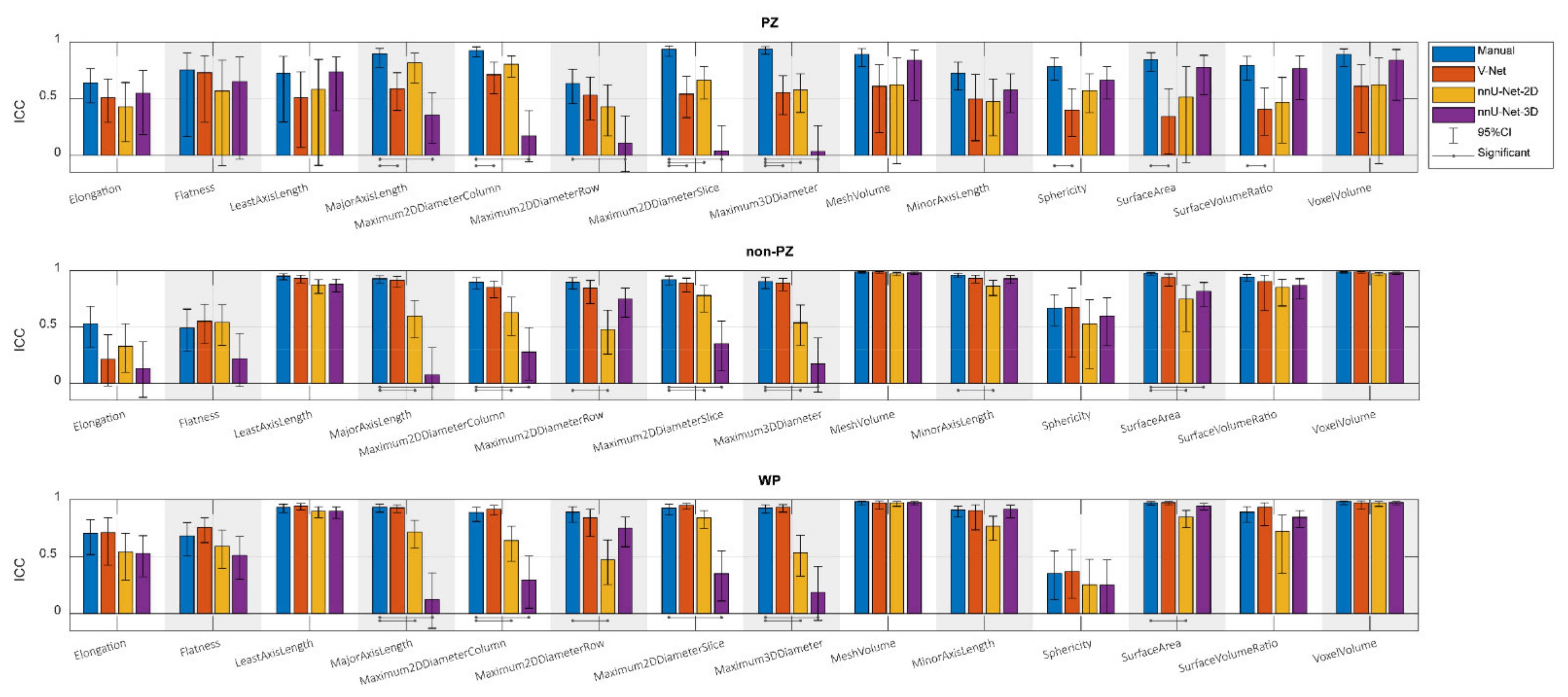
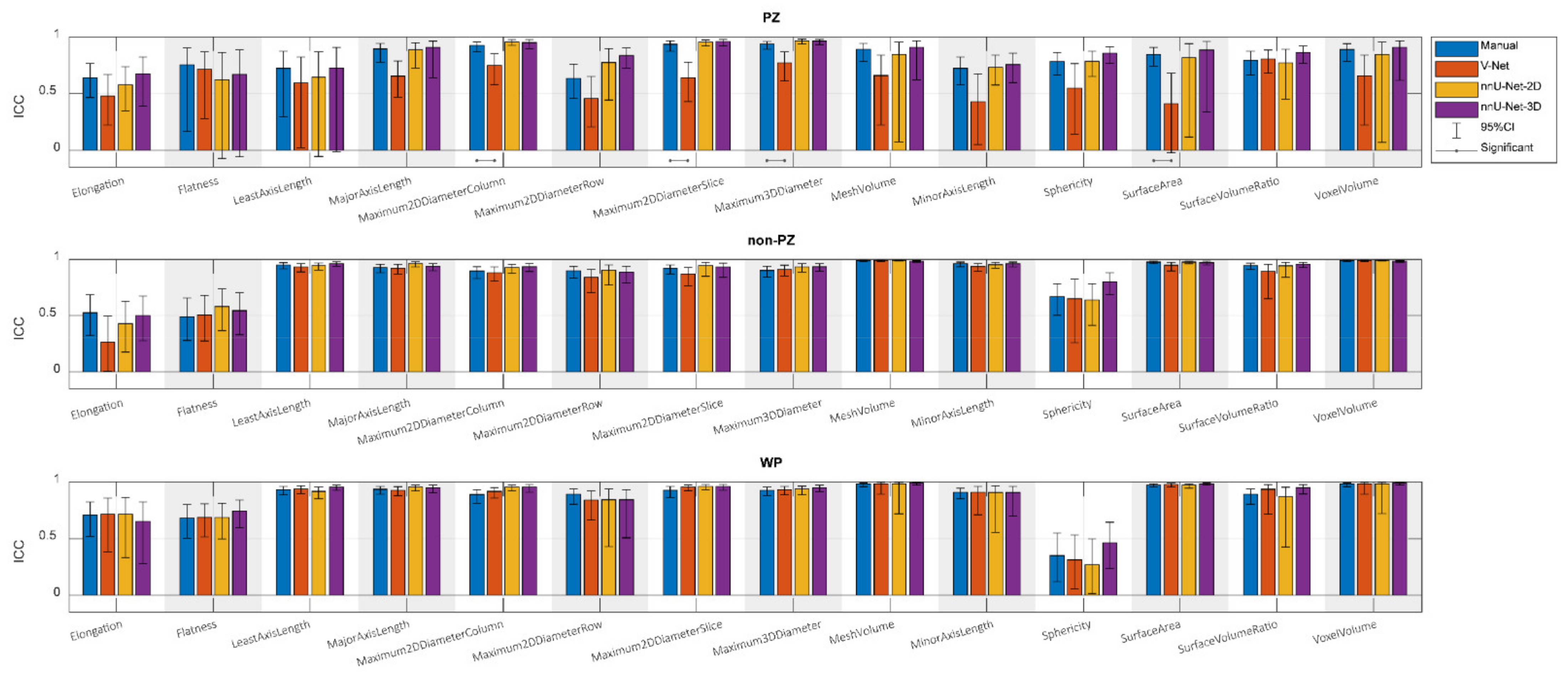
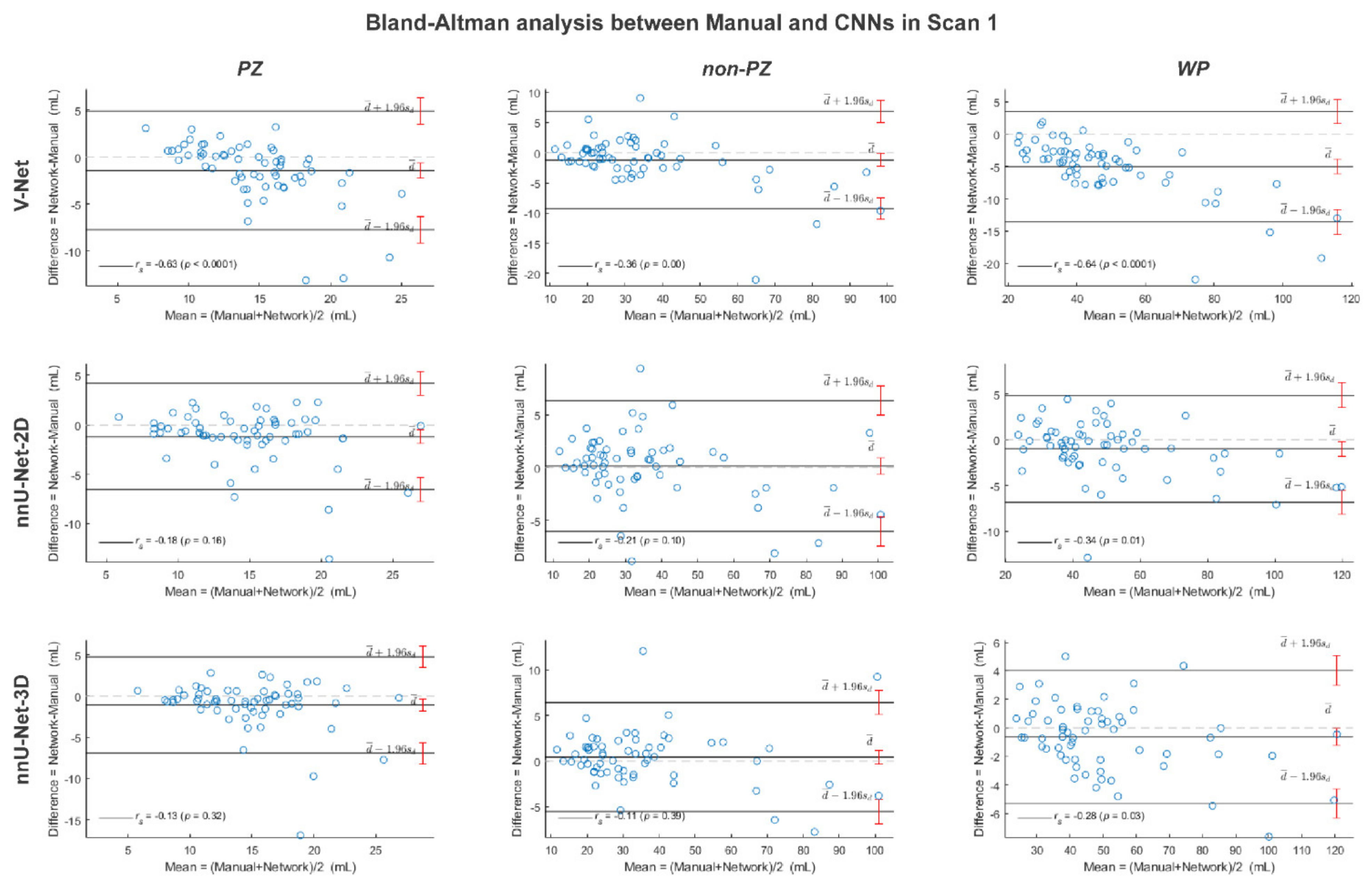
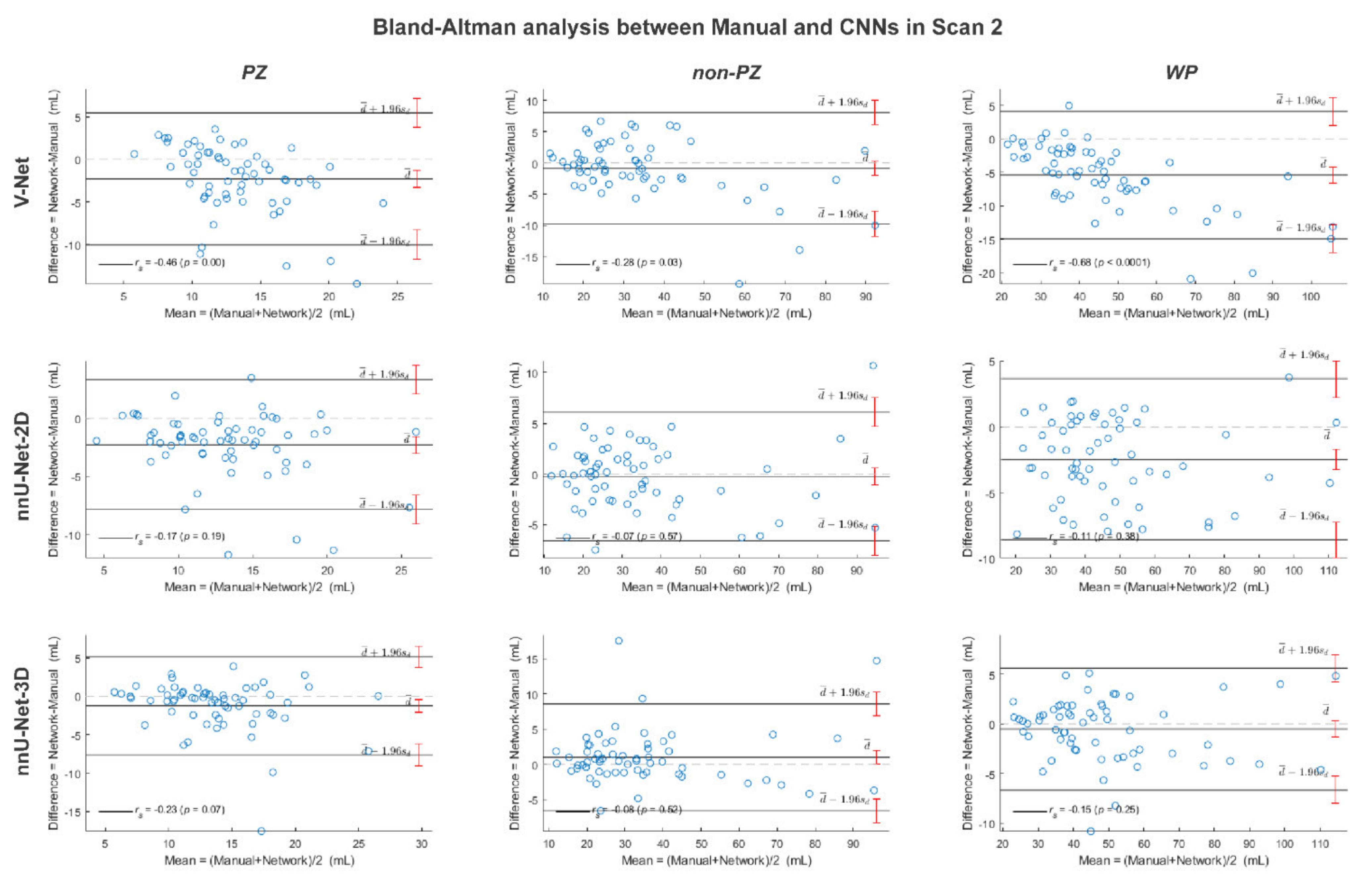
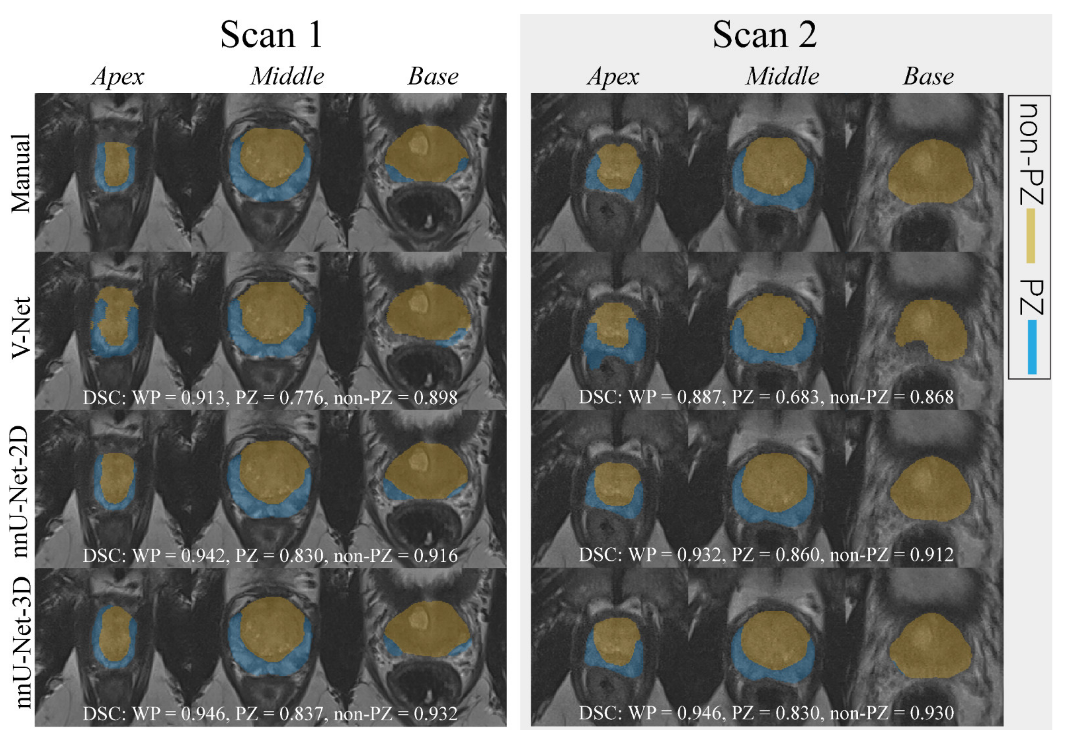
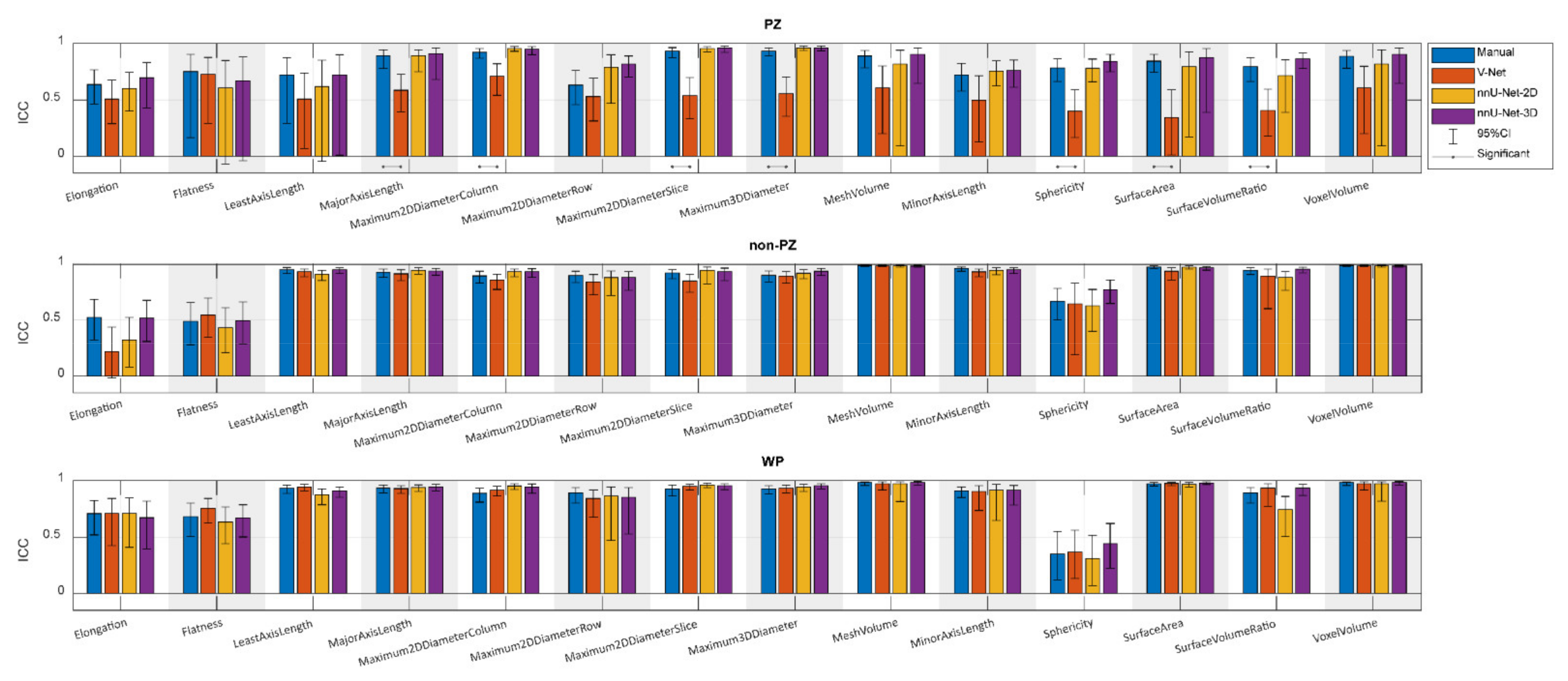
3. Results
4. Discussion
5. Conclusions
Author Contributions
Funding
Institutional Review Board Statement
Informed Consent Statement
Data Availability Statement
Acknowledgments
Conflicts of Interest
Appendix A

References
- Bray, F.; Ferlay, J.; Soerjomataram, I.; Siegel, R.L.; Torre, L.A.; Jemal, A. Global cancer statistics 2018: GLOBOCAN estimates of incidence and mortality worldwide for 36 cancers in 185 countries. CA A Cancer J. Clin. 2018, 68, 394–424. [Google Scholar] [CrossRef] [Green Version]
- Mottet, N.; Bellmunt, J.; Bolla, M.; Briers, E.; Cumberbatch, M.G.; de Santis, M.; Fossati, N.; Gross, T.; Henry, A.M.; Joniau, S.; et al. EAU-ESTRO-SIOG guidelines on prostate cancer. Part 1: Screening, diagnosis, and local treatment with curative intent. Eur. Urol. 2017, 71, 618–629. [Google Scholar] [CrossRef]
- Ahdoot, M.; Wilbur, A.R.; Reese, S.E.; Lebastchi, A.H.; Mehralivand, S.; Gomella, P.; Bloom, J.; Gurram, S.; Siddiqui, M.; Pinsky, P.; et al. MRI-targeted, systematic, and combined biopsy for prostate cancer diagnosis. N. Engl. J. Med. 2020, 382, 917–928. [Google Scholar] [CrossRef] [PubMed]
- Barentsz, J.O.; Richenberg, J.; Clements, R.; Choyke, P.; Verma, S.; Villeirs, G.; Rouviere, O.; Løgager, V.B.; Fütterer, J.J. ESUR prostate MR guidelines 2012. Eur. Radiol. 2012, 22, 746–757. [Google Scholar] [CrossRef] [PubMed] [Green Version]
- Turkbey, B.; Rosenkrantz, A.B.; Haider, M.A.; Padhani, A.; Villeirs, G.; Macura, K.J.; Weinreb, J.C. Prostate imaging reporting and data system version 2.1: 2019 update of prostate imaging reporting and data system version 2. Eur. Urol. 2019, 76, 340–351. [Google Scholar] [CrossRef]
- Weinreb, J.C.; Barentsz, J.O.; Choyke, P.L.; Cornud, F.; Haider, M.A.; Macura, K.J.; Margolis, D.J.; Schnall, M.D.; Shtern, F.; Tempany, C.M.; et al. PI-RADS prostate imaging—Reporting and data system: 2015, version 2. Eur. Urol. 2016, 69, 16–40. [Google Scholar] [CrossRef] [PubMed]
- Fascelli, M.; George, A.K.; Frye, T.; Turkbey, B.; Choyke, P.L.; Pinto, P.A. The role of MRI in active surveillance for prostate cancer. Curr. Urol. Rep. 2015, 16, 42. [Google Scholar] [CrossRef] [PubMed]
- Alberts, A.R.; Roobol, M.J.; Verbeek, J.F.; Schoots, I.G.; Chiu, P.K.; Osses, D.F.; Tijsterman, J.D.; Beerlage, H.P.; Mannaerts, C.K.; Schimmöller, L.; et al. Prediction of high-grade prostate cancer following multiparametric magnetic resonance imaging: Improving the Rotterdam European randomized study of screening for prostate cancer risk calculators. Eur. Urol. 2019, 75, 310–318. [Google Scholar] [CrossRef] [PubMed]
- Patel, P.; Mathew, M.S.; Trilisky, I.; Oto, A. Multiparametric MR imaging of the prostate after treatment of prostate cancer. Radiographics 2018, 38, 437–449. [Google Scholar] [CrossRef]
- Litjens, G.; Debats, O.; Barentsz, J.; Karssemeijer, N.; Huisman, H. Computer-aided detection of prostate cancer in mri. IEEE Trans. Med. Imaging 2014, 33, 1083–1092. [Google Scholar] [CrossRef]
- Girometti, R.; Giannarini, G.; Greco, F.; Isola, M.; Cereser, L.; Como, G.; Sioletic, S.; Pizzolitto, S.; Crestani, A.; Ficarra, V.; et al. Interreader agreement of PI-RADS v. 2 in assessing prostate cancer with multiparametric MRI: A study using whole-mount histology as the standard of reference. J. Magn. Reson. Imaging 2019, 49, 546–555. [Google Scholar] [CrossRef]
- Ruprecht, O.; Weisser, P.; Bodelle, B.; Ackermann, H.; Vogl, T.J. MRI of the prostate: Interobserver agreement compared with histopathologic outcome after radical prostatectomy. Eur. J. Radiol. 2012, 81, 456–460. [Google Scholar] [CrossRef]
- Lemaître, G.; Martí, R.; Freixenet, J.; Vilanova, J.C.; Walker, P.M.; Meriaudeau, F. Computer-aided detection and diagnosis for prostate cancer based on mono and multi-parametric MRI: A review. Comput. Biol. Med. 2015, 60, 8–31. [Google Scholar] [CrossRef] [Green Version]
- Liu, L.; Tian, Z.; Zhang, Z.; Fei, B. Computer-aided detection of prostate cancer with MRI. Acad. Radiol. 2016, 23, 1024–1046. [Google Scholar] [CrossRef] [Green Version]
- Wang, S.; Burtt, K.; Turkbey, B.; Choyke, P.; Summers, R.M. Computer aided-diagnosis of prostate cancer on multiparametric MRI: A technical review of current research. BioMed Res. Int. 2014, 2014, 789561. [Google Scholar] [CrossRef] [PubMed]
- Isensee, F.; Jaeger, P.F.; Kohl, S.A.A.; Petersen, J.; Maier-Hein, K.H. nnU-Net: A self-configuring method for deep learning-based biomedical image segmentation. Nat. Methods 2021, 18, 203–211. [Google Scholar] [CrossRef]
- Khan, Z.; Yahya, N.; Alsaih, K.; Ali, S.S.A.; Meriaudeau, F. Evaluation of deep neural networks for semantic segmentation of prostate in T2W MRI. Sensors 2020, 20, 3183. [Google Scholar] [CrossRef]
- Milletari, F.; Navab, N.; Ahmadi, S.-A. V-net: Fully convolutional neural networks for volumetric medical image segmentation. In Proceedings of the 2016 Fourth International Conference on 3D Vision (3DV), Stanford, CA, USA, 25–28 October 2016; pp. 565–571. [Google Scholar] [CrossRef] [Green Version]
- Wang, B.; Lei, Y.; Tian, S.; Wang, T.; Liu, Y.; Patel, P.; Jani, A.B.; Mao, H.; Curran, W.J.; Liu, T.; et al. Deeply supervised 3D fully convolutional networks with group dilated convolution for automatic MRI prostate segmentation. Med. Phys. 2019, 46, 1707–1718. [Google Scholar] [CrossRef] [PubMed]
- Zavala-Romero, O.; Breto, A.L.; Xu, I.R.; Chang, Y.-C.C.; Gautney, N.; Pra, A.D.; Abramowitz, M.C.; Pollack, A.; Stoyanova, R. Segmentation of prostate and prostate zones using deep learning. Strahlenther Onkol. 2020, 196, 932–942. [Google Scholar] [CrossRef] [PubMed]
- Schelb, P.; Kohl, S.; Radtke, J.P.; Wiesenfarth, M.; Kickingereder, P.V.; Bickelhaupt, S.; Bonekamp, D. Classification of cancer at prostate MRI: Deep learning versus clinical PI-RADS assessment. Radiology 2019, 293, 607–617. [Google Scholar] [CrossRef]
- Schwier, M.; van Griethuysen, J.; Vangel, M.G.; Pieper, S.; Peled, S.; Tempany, C.; Aerts, H.J.W.L.; Kikinis, R.; Fennessy, F.M.; Fedorov, A. Repeatability of multiparametric prostate MRI radiomics features. Sci. Rep. 2019, 9, 9441. [Google Scholar] [CrossRef]
- Chirra, P.; Leo, P.; Yim, M.; Bloch, B.N.; Rastinehad, A.R.R.; Purysko, A.; Rosen, M.; Madabhushi, A.; Viswanath, S. Multisite evaluation of radiomic feature reproducibility and discriminability for identifying peripheral zone prostate tumors on MRI. J. Med. Imaging 2019, 6, 024502. [Google Scholar] [CrossRef]
- Lu, H.; Parra, N.A.; Qi, J.; Gage, K.; Li, Q.; Fan, S.; Feuerlein, S.; Pow-Sang, J.; Gillies, R.; Choi, J.W.; et al. Repeatability of quantitative imaging features in prostate magnetic resonance imaging. Front. Oncol. 2020, 10, 551. [Google Scholar] [CrossRef] [PubMed]
- Scalco, E.; Belfatto, A.; Mastropietro, A.; Rancati, T.; Avuzzi, B.; Messina, A.; Valdagni, R.; Rizzo, G. T2w-MRI signal normalization affects radiomics features reproducibility. Med. Phys. 2020, 47, 1680–1691. [Google Scholar] [CrossRef] [PubMed]
- The Norwegian Directorate of Health. Prostatakreft. Available online: https://www.helsedirektoratet.no/pakkeforlop/prostatakreft (accessed on 31 August 2021).
- Yushkevich, P.A.; Piven, J.; Hazlett, H.C.; Smith, R.G.; Ho, S.; Gee, J.C.; Gerig, G. User-guided 3D active contour segmentation of anatomical structures: Significantly improved efficiency and reliability. NeuroImage 2006, 31, 1116–1128. [Google Scholar] [CrossRef] [PubMed] [Green Version]
- Ronneberger, O.; Fischer, P.; Brox, T. U-net: Convolutional networks for biomedical image segmentation. In International Conference on Medical Image Computing and Computer-Assisted Intervention; Springer: Cham, Switzerland, 2015; pp. 234–241. [Google Scholar] [CrossRef] [Green Version]
- Paszke, A.; Gross, S.; Massa, F.; Lerer, A.; Bradbury, J.; Chanan, G.; Killeen, T.; Lin, Z.M.; Gimelshein, N.; Antiga, L.; et al. PyTorch: An imperative style, high-performance deep learning library. Adv. Neural Inf. Process. Syst. 2019, 32, 8026–8037. [Google Scholar]
- Van Griethuysen, J.J.M.; Fedorov, A.; Parmar, C.; Hosny, A.; Aucoin, N.; Narayan, V.; Beets-Tan, R.G.H.; Fillion-Robin, J.-C.; Pieper, S.; Aerts, H.J.W.L. Computational radiomics system to decode the radiographic phenotype. Cancer Res. 2017, 77, e104–e107. [Google Scholar] [CrossRef] [Green Version]
- Pyradiomics Community. Shape Features (3D). Available online: https://pyradiomics.readthedocs.io/en/v3.0/features.html#module-radiomics.shape (accessed on 14 January 2021).
- Wang, Y.; Tadimalla, S.; Rai, R.; Goodwin, J.; Foster, S.; Liney, G.; Holloway, L.; Haworth, A. Quantitative MRI: Defining repeatability, reproducibility and accuracy for prostate cancer imaging biomarker development. Magn. Reson. Imaging 2021, 77, 169–179. [Google Scholar] [CrossRef] [PubMed]
- Sunoqrot, M.R.S.; Selnæs, K.M.; Sandsmark, E.; Nketiah, G.A.; Zavala-Romero, O.; Stoyanova, R.; Bathen, T.F.; Elschot, M. A quality control system for automated prostate segmentation on T2-weighted MRI. Diagnostics 2020, 10, 714. [Google Scholar] [CrossRef]
- Klein, S.; van der Heide, U.A.; Lips, I.; van Vulpen, M.; Staring, M.; Pluim, J.P.W. Automatic segmentation of the prostate in 3D MR images by atlas matching using localized mutual information. Med. Phys. 2008, 35, 1407–1417. [Google Scholar] [CrossRef] [PubMed]
- McGraw, K.O.; Wong, S.P. Forming inferences about some intraclass correlation coefficients. Psychol. Methods 1996, 1, 30–46. [Google Scholar] [CrossRef]
- Shrout, P.E.; Fleiss, J.L. Intraclass correlations: Uses in assessing rater reliability. Psychol. Bull. 1979, 86, 420–428. [Google Scholar] [CrossRef]
- Stolarova, M.; Wolf, C.; Rinker, T.; Brielmann, A. How to assess and compare inter-rater reliability, agreement and correlation of ratings: An exemplary analysis of mother-father and parent-teacher expressive vocabulary rating pairs. Front. Psychol. 2014, 5, 509. [Google Scholar] [CrossRef] [PubMed] [Green Version]
- Jones, M.C. Nonparametric statistical inference, 3rd edn by J. D. Gibbons, S. Chakraborti. J. R. Stat. Soc. Ser. A 1993, 156, 503. [Google Scholar] [CrossRef]
- Benjamini, Y.; Hochberg, Y. Controlling the false discovery rate: A practical and powerful approach to multiple testing. J. R. Stat. Soc. Ser. B 1995, 57, 289–300. [Google Scholar] [CrossRef]
- Bland, J.M.; Altman, D.G. Statistical methods for assessing agreement between two methods of clinical measurement. Lancet 1986, 1, 307–310. [Google Scholar] [CrossRef]
- Cannon, G.W.; Getzenberg, R.H. Biomarkers for benign prostatic hyperplasia progression. Curr. Urol. Rep. 2008, 9, 279–283. [Google Scholar] [CrossRef] [Green Version]
- Cary, K.C.; Cooperberg, M.R. Biomarkers in prostate cancer surveillance and screening: Past, present, and future. Ther. Adv. Urol. 2013, 5, 318–329. [Google Scholar] [CrossRef] [Green Version]
- Nordström, T.; Akre, O.; Aly, M.; Grönberg, H.; Eklund, M. Prostate-specific antigen (PSA) density in the diagnostic algorithm of prostate cancer. Prostate Cancer Prostatic Dis. 2018, 21, 57–63. [Google Scholar] [CrossRef]
- Loeb, S.; Kettermann, A.; Carter, H.B.; Ferrucci, L.; Metter, E.J.; Walsh, P.C. Prostate volume changes over time: Results from the Baltimore longitudinal study of aging. J. Urol. 2009, 182, 1458–1462. [Google Scholar] [CrossRef] [Green Version]
- Al-Khalil, S.; Ibilibor, C.; Cammack, J.T.; de Riese, W. Association of prostate volume with incidence and aggressiveness of prostate cancer. Res. Rep. Urol. 2016, 8, 201–205. [Google Scholar] [CrossRef] [Green Version]
- Benson, M.C.; Whang, I.S.; Pantuck, A.; Ring, K.; Kaplan, S.A.; Olsson, C.A.; Cooner, W.H. Prostate specific antigen density: A means of distinguishing benign prostatic hypertrophy and prostate cancer. J. Urol. 1992, 147, 815–816. [Google Scholar] [CrossRef]
- Osman, M.; Shebel, H.; Sankineni, S.; Bernardo, M.L.; Daar, D.; Wood, B.; Pinto, P.A.; Choyke, P.L.; Turkbey, B.; Agarwal, H.K. Whole prostate volume and shape changes with the use of an inflatable and flexible endorectal coil. Radiol. Res. Pr. 2014, 2014, 903747. [Google Scholar] [CrossRef] [Green Version]
- Chang, T.-H.; Lin, W.-R.; Tsai, W.-K.; Chiang, P.-K.; Chen, M.; Tseng, J.-S.; Chiu, A.W. Zonal adjusted PSA density improves prostate cancer detection rates compared with PSA in Taiwanese males with PSA < 20 ng/ml. BMC Urol. 2020, 20, 151. [Google Scholar] [CrossRef]
- Kalish, J.; Cooner, W.H.; Graham, S.D. Serum PSA adjusted for volume of transition zone (PSAT) is more accurate than PSA adjusted for total gland volume (PSAD) in detecting adenocarcinoma of the prostate. Urology 1994, 43, 601–606. [Google Scholar] [CrossRef]
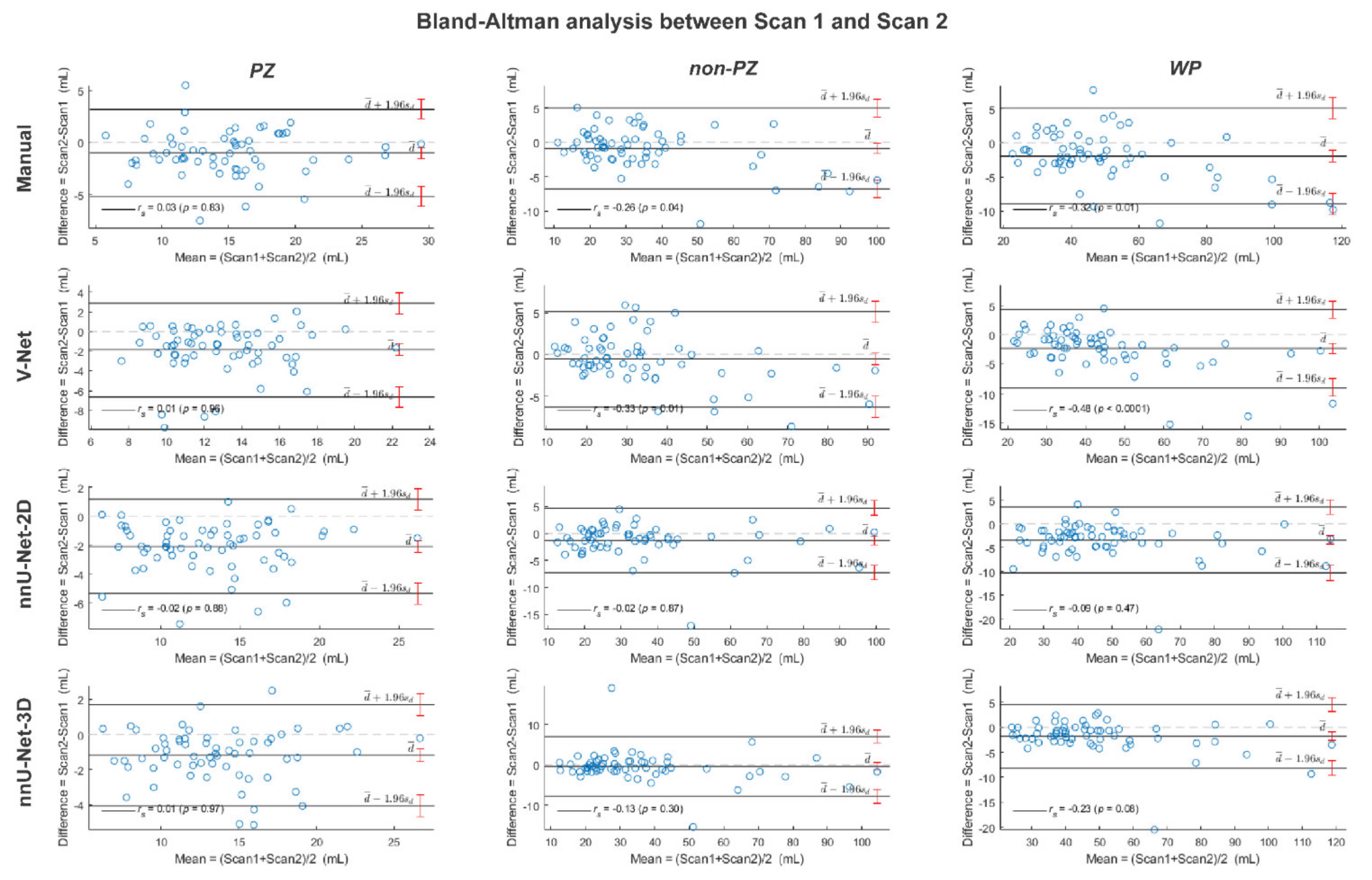
 , while the outliers are denoted by ●.
, while the outliers are denoted by ●.
, while the outliers are denoted by ●.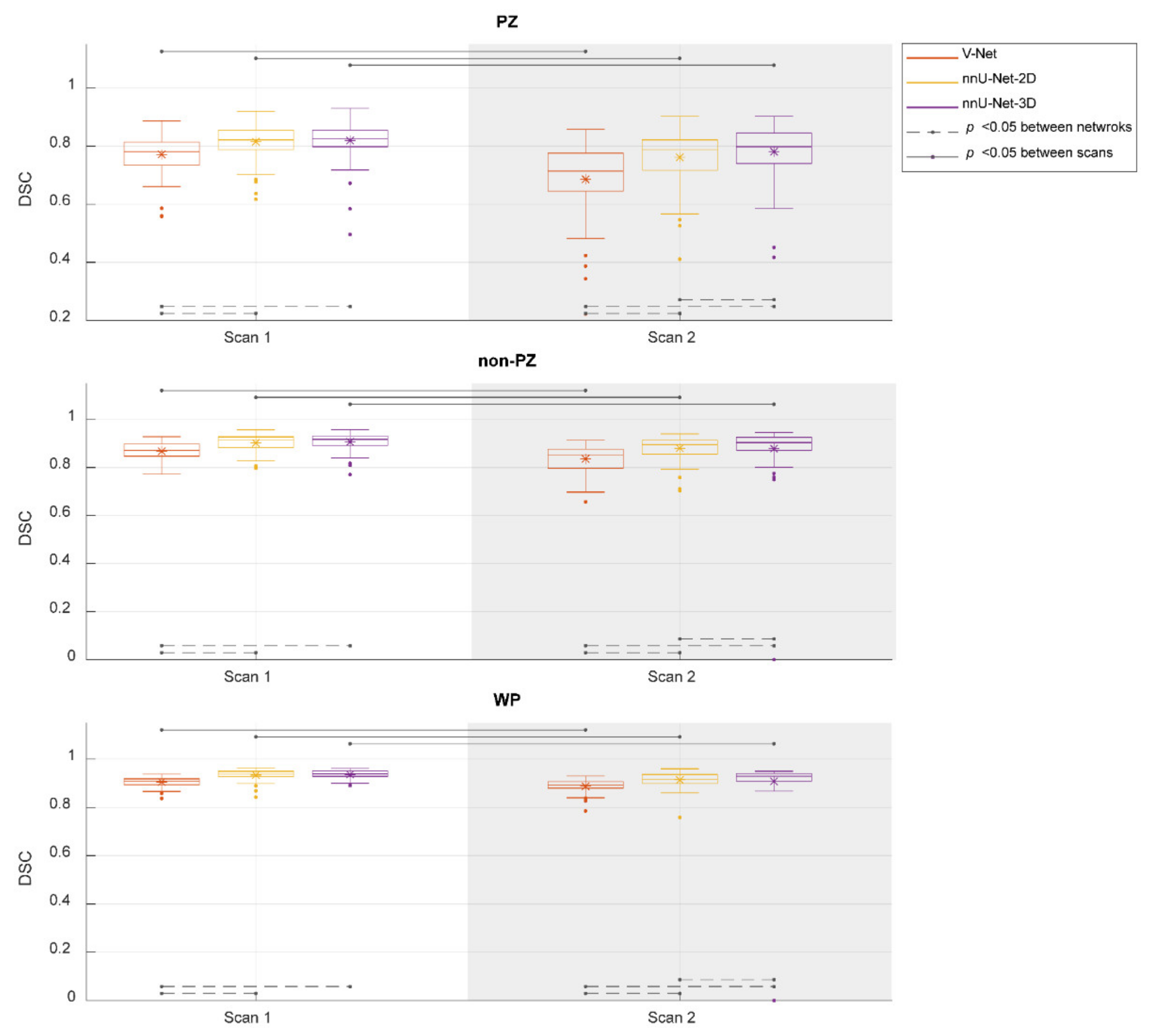
 , while the outliers are denoted by ●.
, while the outliers are denoted by ●.
, while the outliers are denoted by ●.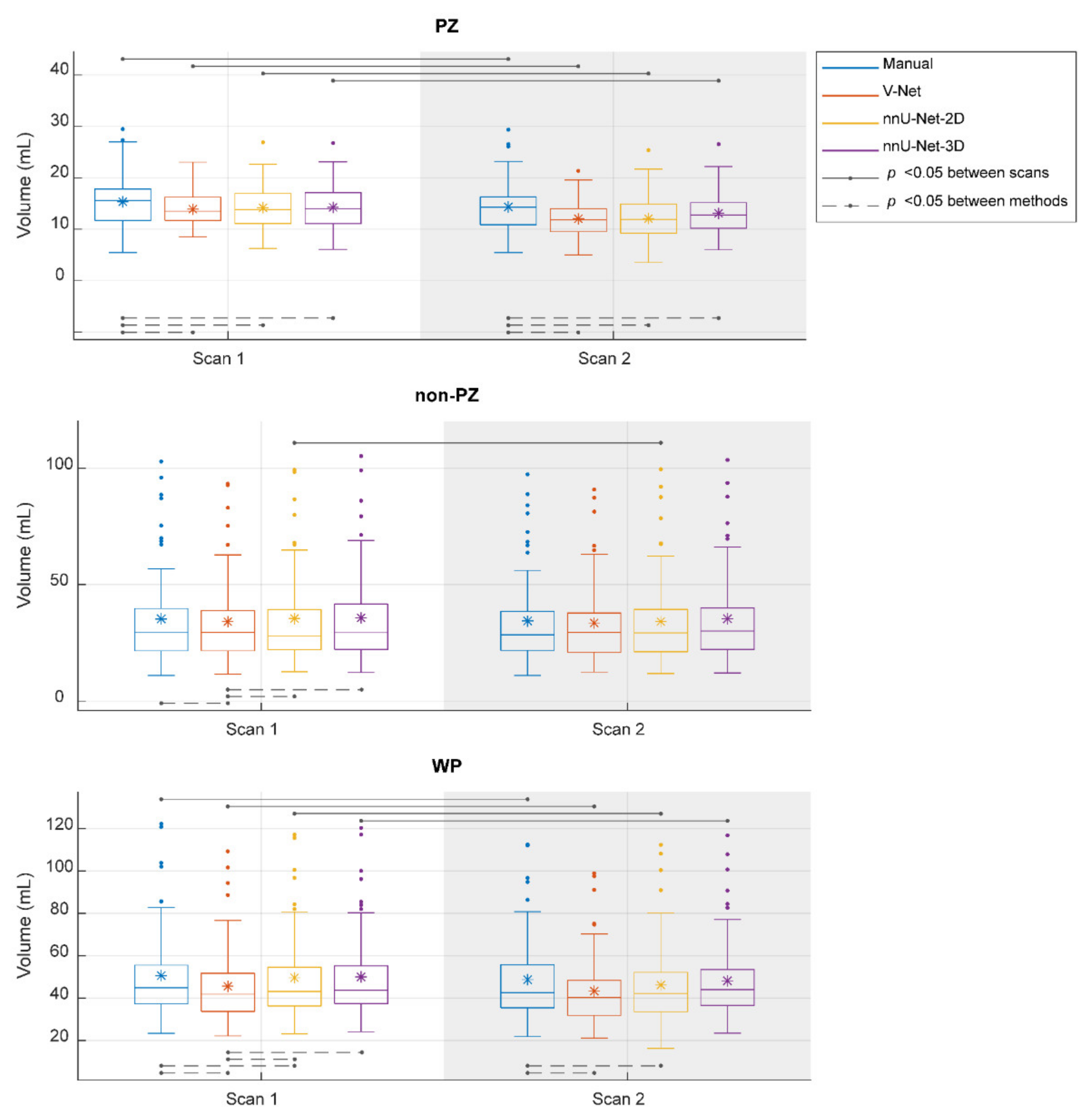

| Investigation Set | Training Set | ||
|---|---|---|---|
| Scan 1 | Scan 2 | ||
| Repetition time (ms) | 4800–8921 | 5660–7740 | 4450–9520 |
| Echo time (ms) | 101–104 | 101–104 | 101–108 |
| Flip angle (degree) | 152–160 | 152–160 | 145–160 |
| Number of averages | 3 | 3–6 | 1–3 |
| Matrix size | 320 × 320–384 × 384 | 320 × 320–384 × 384 | 320 × 320–384 × 384 |
| Slices | 24–30 | 17–24 | 24–34 |
| Slice thickness (mm) | 3 | 3 | 3–3.5 |
| In plane resolution (mm2) | 0.5 × 0.5–0.6 × 0.6 | 0.5 × 0.5–0.6 × 0.6 | 0.5 × 0.5–0.6 × 0.6 |
Publisher’s Note: MDPI stays neutral with regard to jurisdictional claims in published maps and institutional affiliations. |
© 2021 by the authors. Licensee MDPI, Basel, Switzerland. This article is an open access article distributed under the terms and conditions of the Creative Commons Attribution (CC BY) license (https://creativecommons.org/licenses/by/4.0/).
Share and Cite
Sunoqrot, M.R.S.; Selnæs, K.M.; Sandsmark, E.; Langørgen, S.; Bertilsson, H.; Bathen, T.F.; Elschot, M. The Reproducibility of Deep Learning-Based Segmentation of the Prostate Gland and Zones on T2-Weighted MR Images. Diagnostics 2021, 11, 1690. https://doi.org/10.3390/diagnostics11091690
Sunoqrot MRS, Selnæs KM, Sandsmark E, Langørgen S, Bertilsson H, Bathen TF, Elschot M. The Reproducibility of Deep Learning-Based Segmentation of the Prostate Gland and Zones on T2-Weighted MR Images. Diagnostics. 2021; 11(9):1690. https://doi.org/10.3390/diagnostics11091690
Chicago/Turabian StyleSunoqrot, Mohammed R. S., Kirsten M. Selnæs, Elise Sandsmark, Sverre Langørgen, Helena Bertilsson, Tone F. Bathen, and Mattijs Elschot. 2021. "The Reproducibility of Deep Learning-Based Segmentation of the Prostate Gland and Zones on T2-Weighted MR Images" Diagnostics 11, no. 9: 1690. https://doi.org/10.3390/diagnostics11091690