Article

Impact of Lesion Delineation and Intensity Quantisation on the Stability of Texture Features from Lung Nodules on CT: A Reproducible Study

1
Department of Engineering, Università Degli Studi di Perugia, Via Goffredo Duranti 93, 06135 Perugia, Italy
2
Section of Radiation Oncology, Department of Medicine and Surgery, Università Degli Studi di Perugia, Piazza Lucio Severi 1, 06132 Perugia, Italy
3
Department of Mechanical and Aerospace Engineering (DIMEAS), Politecnico di Torino, Corso Duca Degli Abruzzi, 24, 10129 Torino, Italy
4
Unit of Nuclear Medicine, Department of Medical, Surgical and Experimental Sciences, Università Degli Studi di Sassari, Viale San Pietro 8, 07100 Sassari, Italy
5
Section of Nuclear Medicine and Health Physics, Department of Medicine and Surgery, Università Degli Studi di Perugia, Piazza Lucio Severi 1, 06132 Perugia, Italy
*
Author to whom correspondence should be addressed.
Diagnostics 2021, 11(7), 1224; https://doi.org/10.3390/diagnostics11071224
Submission received: 29 May 2021 / Revised: 28 June 2021 / Accepted: 28 June 2021 / Published: 6 July 2021

Abstract

:
Computer-assisted analysis of three-dimensional imaging data (radiomics) has received a lot of research attention as a possible means to improve the management of patients with lung cancer. Building robust predictive models for clinical decision making requires the imaging features to be stable enough to changes in the acquisition and extraction settings. Experimenting on 517 lung lesions from a cohort of 207 patients, we assessed the stability of 88 texture features from the following classes: first-order (13 features), Grey-level Co-Occurrence Matrix (24), Grey-level Difference Matrix (14), Grey-level Run-length Matrix (16), Grey-level Size Zone Matrix (16) and Neighbouring Grey-tone Difference Matrix (five). The analysis was based on a public dataset of lung nodules and open-access routines for feature extraction, which makes the study fully reproducible. Our results identified 30 features that had good or excellent stability relative to lesion delineation, 28 to intensity quantisation and 18 to both. We conclude that selecting the right set of imaging features is critical for building clinical predictive models, particularly when changes in lesion delineation and/or intensity quantisation are involved.

1. Introduction

Lung cancer, excluding skin cancer, is the second most common type of cancer in both genders after prostate cancer in men and breast cancer in women [1,2]. Unfortunately, the overall five-year survival rate of patients with lung cancer is still dismally low (≈18.6%) and far below that of the other types of oncological disorders such as colorectal (≈64.5%), breast (≈89.6%) and prostate (≈98.2%) cancer [2]. The survival rate, however, depends a great deal on the stage of the disease when it is first diagnosed, ranging from a grim ≈5% for distant tumours to ≈56% when the disease is still localized [2].
The effectiveness of lung cancer therapy strongly relies on early diagnosis. Chest radiographies (CXRs), computed tomography (CT), magnetic resonance imaging (MRI), positron emission tomography (PET), cytology sputum and breath analysis represent the currently available detection techniques for lung cancer [3]. Computed tomography, in particular, plays a pivotal role in differentiating benign vs. malignant lung nodules in the early screening phase. However, although CT scans provide valuable information about suspicious lung nodules, their correct interpretation can be a challenging task for the radiologist. In this context, computer-assisted diagnosis may provide a valid support for the radiologist to contribute to the diagnostic process of lung cancer.
In recent years computerised analysis of imaging data (particularly from CT and PET/CT) has shown great promises to improve the management of patients with lung cancer [4,5,6,7,8,9,10]. The rationale behind this paradigm is that the quantitative extraction of imaging parameters from suspicious lesions—particularly shape and texture features—may reveal hidden patterns that would otherwise go unnoticed to the naked eye [11,12]. Furthermore, the extraction of objective, reproducible and standardised imaging parameters helps reduce the intra-observer and inter-observer bias and facilitates tracking changes over time. Radiomics leverages on artificial intelligence techniques and the increasing availability of large, open-access and multicentric datasets of pre-classified cases to infer clinical information about unknown ones (‘population imaging’ approach [13]). Several studies have underlined the potential benefit of radiomics for clinical problem-solving in lung cancer, such as prediction of malignancy [14,15,16], histological subtype [17,18,19], prognosis [20,21,22] and response to treatment [23,24,25] (see also Figure 1 for an overview of potential applications).
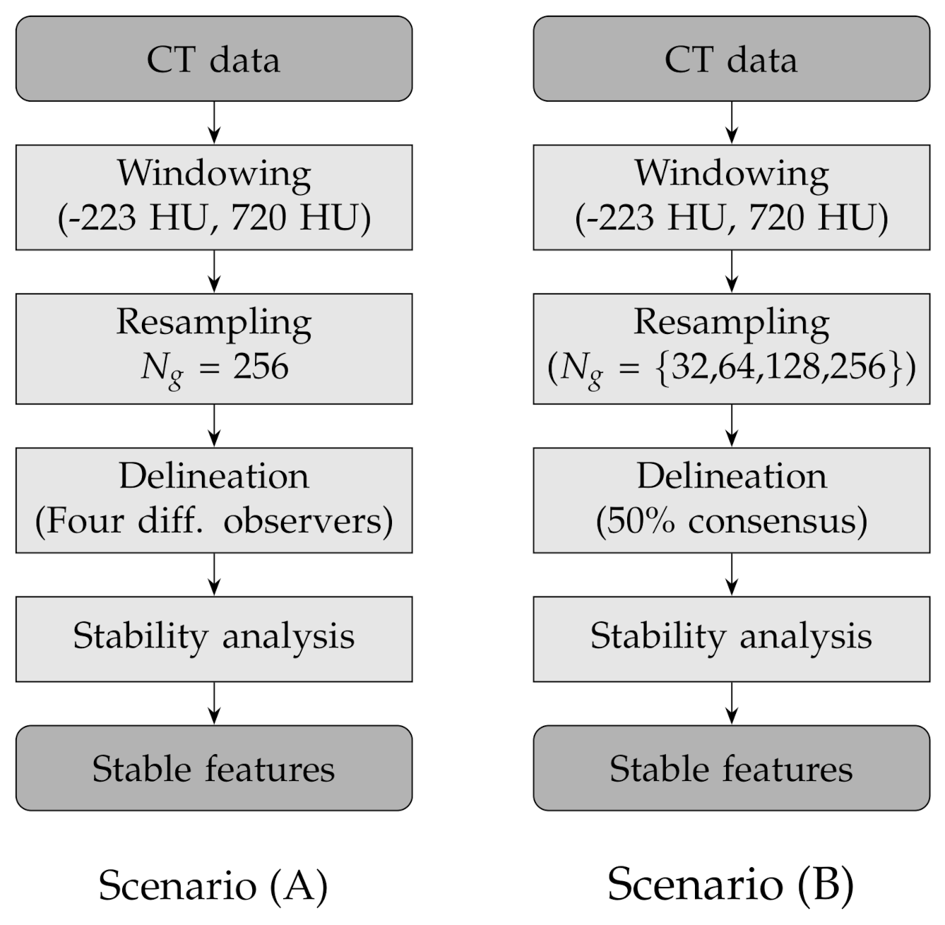
The radiomics pipeline consists of six steps [26]: (1) acquisition, (2) pre-processing, (3) segmentation (also referred to as delineation), (4) feature extraction, (5) post-processing and (6) data analysis/model building. The fourth step, which aims at extracting a set of quantitative parameters from the region of interest, is central to the whole process and various studies have shown that steps 1–3 can have significant impact on feature extraction [27,28,29,30,31,32]. A current major research focus is therefore the assessment of the stability of radiomics features to changes in image acquisition settings, signal pre-processing and lesion delineation (see Traverso et al. [33] for a general review on the subject).
In particular, the repeatability and reproducibility of radiomics features from lung lesions on CT has been investigated in a number of recent works. In [34] Balagurathan et al. evaluated the test-retest reproducibility of texture and non-texture features from chest CT scans to two consecutive acquisitions (on the same patient) taken within 15 min from one another. Of the 329 features included in their study, they found that 29 (i.e., approximately one in eleven) had a concordance correlation coefficient (CCC) > 0.9 . The study by Seung-Hak et al. [35] addressed the impact of voxel geometry and intensity quantisation on 260 lung nodules at CT; in this case the results indicated that nine of the 252 features investigated had high reproducibility among the different experimental settings. As for stability to lesion segmentation, Kalpathy-Cramer et al. [36] investigated 830 radiomics features from CT scans of pulmonary nodules at CT and determined that 68% of them had CCC 0.75 . Parmar et al. [37] compared the variability of radiomics features extracted from automatically segmented lesions (3D-Slicer) with that of features from manually-segmented ones and found higher reproducibility in the first case. Owens et al. [38] examined the repeatability of 40 radiomics features from ten CT scans of non-small lung cancer to manual and semi-automatic lesion delineation consequent to intra-observer, inter-observer and inter-software variability. Similarly to [37], they concluded that semi-automatic lesion delineation can provide better reproducible radiomics features than manual segmentation. Tunali et al. [39] assessed the repeatability relative to the test-retest of 264 radiomics features from the peritumoural area of lung lesions and their stability to nine semi-automated lesion segmentation algorithms. They determined an unlikely response between the different classes of texture features investigated with first-order features generally showing better stability than the other groups. More recently, Haarburger et al. [40] evaluated the stability of 89 shape and texture features to manual and automatic lesion delineation, finding that 84% of the features investigated had intra-class correlation coefficient (ICC) > 0.8 .
One common shortcoming in the available studies, however, is that most of them are based on proprietary datasets (with the notable exception of [40]) and custom feature extraction routines, all of which renders the results difficult to reproduce. In this work we investigated the stability of 88 textural features from CT scans of lung lesions to delineation and intensity quantisation. To guarantee reproducibility we based our study on a public dataset (LIDC-IDRI [41]) and on feature extraction routines from an open-access package (PyRadiomics [42]). Furthermore, we made all the code used for the experiments freely available to the public for future comparisons and evaluations. Our results identified 30 features that had good or excellent stability to lesion delineation, 28 to intensity quantisation and 18 to both.

2. Materials and Methods

2.1. Patient Population

The study population included a total of 517 lung lesions (axial diameter = 16.2 ± 11.5 mm (3.2–72.3 mm)) from a cohort of 207 patients (110 males, 97 females, age = 59.0 ± 14.7 year (14–88 year)) who underwent thoracic computed tomography (CT) for lung cancer screening. The data were sourced from the open-access Lung Image Database Consortium collection (LIDC-IDRI [41,43]). Since this is a multicentric dataset, different imaging systems, acquisition protocols and image reconstruction settings were used and included among them are the following: tube voltage 120–140 kV, in-plane pixel spacing 0.53–0.98 mm, slice thickness 0.6–3.0 mm and slice spacing 0.5–3.0 mm. Each nodule was manually annotated by one to five radiologists relative to subtlety (difficulty of detection), internal structure (soft, fluid, fat or air), pattern of calcification (if present), sphericity, margin (sharp vs. poorly defined), degree of lobulation, extent of spiculation, radiographic solidity (solid, non-solid, ground-glass or mixed) and subjective assessment of the likelihood of malignancy (from highly unlikely to highly suspicious). The complete (anonymous) list of the patient IDs along with the main acquisition settings for each scan and that of each nodule with the related annotations are provided as Supplementary Material (scans_metadata.csv, nodules_metadata.csv). Further details about the study population can also be retrieved from the LIDC-IDRI repository either through the pylidc interface or via direct access to the DICOM data (see also Section 2.5 on this point). Scans with incomplete metadata (e.g., lack of patient’s gender and/or age were excluded from our study).

2.2. Image Preprocessing

Pre-processing involved uniform intensity discretisation within a fixed-width window. The original CT signal was first clipped between CT m i n = μ d 2 σ d and CT m a x = μ d + 2 σ d , where μ d , σ d , respectively, represent the mean and standard deviation of the average nodule density in the dataset. The resulting bounds were CT m i n = −583 HU and CT m a x = 137 HU (window level = −223 HU, width = 720 HU). Intensity values below the lower bound or above the upper bound were set to CT m i n or CT m a x , respectively. Uniform signal quantisation was then applied using N g = 32, 64, 128 and 256 discretisation levels, which in terms of bin width corresponded to approximately 23 HU, 11 HU, 6 HU and 3 HU, respectively. No further pre-processing operations such as filtering or spatial resampling/interpolation were applied.

2.3. Feature Extraction

A total of 88 textural features from six classes were included in this study (see Table 1 and Table 2 for the complete list). All the features are compliant with the Imaging Biomarker Standardization Initiative (IBSI [44]); volume-confounded features were not considered in the analysis. For mathematical definitions and formulae we refer the reader to the documentation available in [42]. Grey-level co-occurrence matrix (GLCM), grey level dependence matrix (GLDM) and Grey level size zone matrix (GLSZM) features were all computed using inter-voxel distance δ = 1 and a three-dimensional 26-connectivity voxel neighbourhood. Feature extraction was based on the open-source PyRadiomics package (see also Section 2.5 for further details).

2.4. Experimental Design and Stability Assessment

In order to assess the stability of the texture features to lesion delineation (A) and intensity resampling (B), we considered two experimental scenarios with the following combinations of factors (see also Table 3 and Figure 2 for a round-up):
(A)
Fixed number of quantisation levels ( N g = 256 ) and four lesion delineations per nodule; each delineation was generated by one different observer;
(B)
Number of quantisation levels for intensity resampling N g = 32, 64, 128 and 256 and fixed lesion delineations based on consensus consolidation at 50% agreement level—that is, a voxel was considered in the lesion when at least 50% of the available delineations included that voxel and not in the lesion otherwise.
In the first scenario (A) we limited the analysis to a subset of 206 nodules from 130 patients for which four lesion annotations were available for each nodule (see Figure 3 for an example of different delineation on the same nodule). The observers (raters) are unknown and, due to the multicentric nature of the dataset, they are likely to be different from one nodule to another. In the second scenario (B), we had four different (but fixed) quantisation levels, which can be considered equivalent to different raters (Figure 4).
In both cases the assessment of feature stability was based on the average Symmetric Mean Absolute Percentage Error (sMAPE [45,46]). Specifically, for each nodule and set of raters (delineation or intensity resampling), we computed the average sMAPE for all the observation pairs and averaged the results over the whole population. In formulas, denoted with x i j the reading on the i-th nodule by the j-th rater the by-nodule sMAPE S i is defined as follows:
S i = 1 | P ( [ J ] , 2 ) | ( f , t ) P ( [ J ] , 2 ) x ^ i x i x ^ i + x i × 100
where J is the number of raters and P ( [ J ] , 2 ) denotes the 2-ordered subsets of [ J ] , that is, all the pairwise permutations of { 1 , , J } . In other words, S i computes the average sMAPE between pairs of readings each given by two observers, where one of the observers is being alternatively considered the reference (therefore returning the ‘true’ value x i ) or the estimator (giving the “forecast” value x ^ i ). One advantage of S i is that it counteracts the intrinsic asymmetry—despite its name—of the sMAPE [46]. Furthermore, since it is customary in the practice [45], we omitted the division by two from the summand’s denominator in Equation (1), which forces S i to have values in [ 0 , 100 ] . Finally, we obtained the overall stability measure S by averaging S i over all the nodules:
S = 1 N i = 1 N S i
where N is the total number of nodules. For an easier interpretation of the results we established a qualitative scale of feature stability in four grades as detailed in Table 4. A discussion about the use of sMAPE compared with other stability measures is also presented in Section 4.

2.5. Implementation, Execution and Reproducible Research

The experiments were carried out on a laptop PC with Intel ® Core i7-9750H CPU @ 2.60 GHz, 32 GB RAM, NVIDIA Quadro T1000 (4 GB) graphics card and Windows 10 Pro 64-bit operating system. The implementation was based on Python 3.8.6, with functions from dicom-parser 0.1.6 [47], NumPy 1.18.5 [48], Pandas 1.1.3 [49,50], pylidc 0.2.2 [51,52], pynrrd 0.4.2 [53] and Py-Radiomics 3.0.1 [42,54]. For reproducible research purposes, all the code and settings are available on the following GitHub repository: https://github.com/bianconif/stability_radiomics_features_lung_ct, accessed on 3 July 2021.

3. Results

Table 5, Table 6, Table 7, Table 8, Table 9 and Table 10 summarise the results of the experiments. As it can be observed, of the 88 features considered in the study, 18 showed good or excellent stability (defined as S 
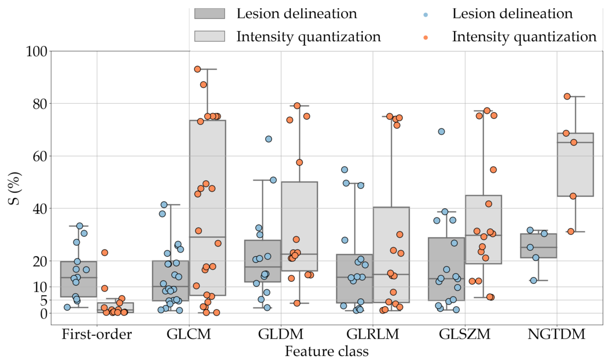
10%) relative to both lesion delineation and intensity quantisation. Broken down by class, the number (percentages) of features with at least good stability relative to both delineation and intensity quantisation were: 4/13 (≈31%) for first-order features, 6/24 (33%) for GLCM features, 1/14 (≈7%) for GLDM features, 5/16 (31%) for GLRLM features and 2/16 (≈13%) for GLSZM features, whereas none of the five NGTDM features achieved at least good stability relative to both conditions.
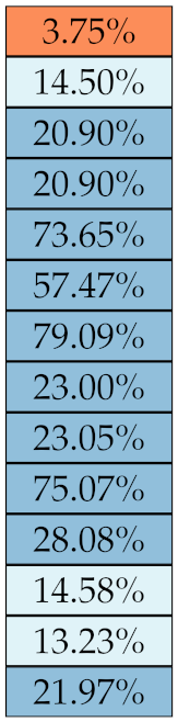
If we examine the results by class of features we observe that those of the first-order (except Uniformity) all had at least good repeatability relative to intensity quantisation (this is evident also from Figure 5). This is, of course, what we expected, as these features (excluding Entropy and Uniformity) are by definition independent on signal quantisation—apart from numerical round-off errors. It is also no surprise that Entropy and Uniformity (Respectively defined as ‘Discretised intensity entropy’ and ‘Discretised intensity uniformity’ in the Image Biomarker Standardisation Initiative [55]) exhibited the highest relative error (9.40% and 23.05%, respectively), for they depend—by definition—on the number of quantisation levels used. Under the currently accepted formulations [42,55], Entropy and Uniformity have values in [ 0 , log 2 ( N g ) ] and [ 1 / N g , 1 ] , respectively, which sets into evidence the dependency on N g . As for stability to lesion delineation, it emerged that Max was the most stable feature. This is coherent with tissue density being usually highest in the central area of the lesion, which is also the part of the tissue that most observers would include in the delineation. The other parameters that had good to excellent stability were Entropy, Range and Min.
For the other classes, Figure 5 indicates that the data about intensity quantisation were, on the whole, more dispersed than those about lesion resampling. Features from GLCM generally proved more resilient to changes in lesion delineation (half of them had S 10.0 ) than intensity resampling (only seven features out of 24 reached at least good stability). This is, again, coherent with the GLCM definition depending heavily on the number of quantisation levels.
Similar arguments hold for the other classes of texture features. In particular, GLDM produced very few stable features: Only three of them showed at least good stability to lesion delineation and only one to intensity resampling. It is worth recalling that GLDM is based on the concept of ‘depending’ voxels [42,56]; that is, a neighbouring voxel is considered dependent on the central voxel if the absolute difference between the intensity values of the two is below a user-defined threshold α . For the threshold value we used the default PyRadiomics settings ( α = 0 ) and this may have had an effect—possibly negative—on the stability of this group of features. Likewise, GLSZM features were highly sensitive to signal quantisation too, which is again logical given the definition of GLSZM. Recall that this is based on sets of connected voxels (grey zones) sharing the same grey-level intensity; consequently, changes in signal quantisation are likely to produce different grey-zones, with fewer quantisation levels resulting in larger grey-zones and vice versa. This inevitably reflects on the feature values.
Notably, none of the NGTDM features proved resilient enough to both lesion delineation and intensity resampling (Table 10). As for lesion delineation, only Busyness and Strength attained excellent and good stability, respectively, whereas Coarseness was the only feature with good stability to intensity resampling. Consider that NGTDM [42,57] estimates the joint probability between the intensity level at one voxel and the average intensity difference among its neighbour voxels; we speculate that changing the number of resampling levels ( N g ) may alter the joint distribution and this could explain the poor stability to signal quantisation.

4. Discussion

Radiomics has attracted increasing research interest in recent years as a possible means to assist physicians in clinical decision making. Potential applications in pulmonary imaging include, in particular, detection and assessment of suspicious lung nodules; prediction of histological subtype, prognosis and response to treatment. The radiomics workflow involves six steps, each of which is sensitive to a number of settings and parameters. Stability of radiomics features to these settings is therefore critical for guaranteeing reproducibility and consistency across multiple institutions.
Regarding stability to lesion delineation, a comparison with previously published works indicate that our results are by and large in agreement with what was reported by Haarburger et al. [40] concerning first-order, GLDM, GLSZM and GLRLM features. However, our study indicated lower stability of GLCM and NGTDM features than reported in [40]. One possible explanation of this discrepancy might be that the bin width used here (≈3 HU) was different than adopted in [40] (25 HU). In [34] Balagurunatan et al. found 29 features stable to lesion delineation, of which five were also investigated in the present work. Our findings show partial overlap with [34]: first-order Entropy and GLRLM RLN achieved good stability in both studies; on the other hand, GLCM Contrast, GLRLM GLN and RLN were stable in [34] but not here. As for intensity quantisation, Lee et al. [35] reported three highly stable (ICC > 0.7 ) first-order features (Max, Min and Entropy), which confirmed their performance ( S 10 % ) in our experiments, and two GLCM features (DiffEnt and Homogeneity—equivalent to ID); however, the reproducibility of the latter two was only moderate (DiffEnt) and poor (ID) in our study. In Shafiq-Ul-Hassan et al.’s phantom study [58], 11 texture features panned out as highly stable and defined as percent coefficient of variation (%COV) below 30%. Out of them, the ones directly comparable with the present work are first-order Uniformity (indicated as Energy in [58]); GLCM InvVar and JointAvg; GLRLM GLN and RLN; and NGTDM Coarseness and Strength. Among these only the GLCM ones attained good stability in our experiments, albeit the threshold for ‘goodness’ adopted in [58] (%COV < 30%) was far more generous than can be used here ( S 10 % ).
One much debated question in radiomics is whether intensity resampling should be absolute or relative [59]. In the first case, the window bounds are determined a priori and are invariable across different scans and ROIs, whereas in the second case they are relative to the region of interest. When intensity values represent quantities with the same physical meaning across different scans (such as Hounsfield Units—assuming there are no calibration errors) the use of absolute resampling seems logical [42,60] and this was the decision made here. As detailed in Section 2.2, we determined the window bounds based on the actual distribution of the intensity values in the whole dataset, but other choices such as mediastinal (W:350, L:50) or lung (W:1500, L:−600) window would be reasonable options as well. Notably, our results indicate that changes in intensity quantisation had little consequence on most of the first-order features; whereas the effect on the other classes was generally stronger and with much larger intra-class variability (see Figure 5). This suggests that particular care should be taken in the selection of texture features different than first-order when changes in signal quantisation are involved.
Another methodological point that requires further attention is what figure of merit should be used for assessing feature stability. Althought Intra-class Correlation Coefficient (ICC) is the common practice in the literature [35,37,38,40], we did not think this was the correct choice here. There are two reasons behind this observation. First, ICC assumes a statistical model where the true scores are normally distributed among the study population [61], but of course this is not guaranteed. Second, in a multicentric study much of the inter-subject variance may come from differences in parameters that are hard to control, such as voxel size, slice thickness, tube voltage, etc., all of which may have unknown and unpredictable effects on the estimated ICC. In order to avoid these potential problems we based our evaluation on a direct measurement of intra-rater difference at the nodule level, as for instance used in Varghese et al.’s phantom study [29], and averaged the result over the whole population. The resulting S (Equation (1)–(2)) avoids the unpredictable effects consequent to between-nodule differences in the acquisition settings; furthermore, it has a straightforward interpretation (values are bound between 0% and 100%) and does not rely on any assumptions on the distribution of the underlying data.
Focussing on the potential implications of radiomics in clinical decision making, one major problem related to the lack of feature stability is that the results are difficult to reuse across multiple centres. If one centre determines that having a certain feature value above a given threshold is predictive of malignancy in lung nodule screening, a second one can reuse that result only if (a) the features are computed using the same settings or (b) the features are stable enough. Concerning intensity quantisation, of course one sensible approach would be to stick to one value ( N g = 256 is a common choice [16,62,63,64]) in order to have comparable data. However, for some features simple mathematical transformations could be applied to make the features independent of the number of quantisation levels (see for instance Appendix A). In order to avoid or reduce the inter-observer bias related to manual lesion delineation, automated and semi-automated methods offer great promises in terms of speed, accuracy and repeatability [65]. Previous studies have shown that semi-automated segmenters can improve on manual delineation and generate more reproducible radiomics features [37,38].

5. Conclusions and Future Work

In recent years, the extraction of quantitative imaging features from lung lesions on CT has attracted increasing research interest as a potential tool to improve diagnosis, risk stratification and the follow-up of lung cancer. Still, the applicability of radiomics across multiple institutions and on large populations of patients depends a great deal on the robustness of the image features to changes in the acquisition settings, preprocessing procedures and lesion delineation methods. In this context the objective of this work was to evaluate the impact of lesion delineation and intensity quantisation on the stability of texture features extracted from suspicious lung nodules on CT scans. Specifically, we assessed the robustness of 88 texture features from six classes: first-order, GLCM, GLDM, GLRLM, GLSZM and NGTDM. For reproducible research purposes, we carried out the experiments on a public dataset of lung nodules (LIDC-IDRI) and employed open-source tools (Python and PyRadiomics) for feature extraction. Implementation settings and code are also available to the public for future comparisons and evaluation.
The results indicate that the impact of changes in lesion delineation and intensity quantisation was important: of the 88 texture features included in the study, only 18 showed good stability ( S 10 % ) relative to both types of change. These findings suggest caution when it comes to building predictive models involving CT features obtained with different quantisation schemes and/or affected by contour variability. From a clinical standpoint, our results are useful as they identify a set of stable CT texture features that can contribute to the diagnosis of lung cancer. This is very important for the discovery of robust imaging biomarkers that may help characterise lung lesions, particularly, in those cases where the anatomical site or the clinical presentation of the patient rule out other invasive methods (e.g., biopsy).
The present investigation indicates different directions for future research. In confirming previous studies [58], we found that most texture features were sensitive to intensity quantisation of the CT signal. This suggests (a) that the mathematical formulations of these features may need to be revised in order to remove such dependency (as for instance proposed in Appendix A) and/or (b) that the number of quantisation level should be defined/recommended in internationally-accepted guidelines (standardisation). Similarly, the effects of intra-observer and inter-observer variability in lesion delineation could be reduced by recurring to automated and semi-automated segmentation procedures. As pointed out in [35], this is particularly critical in lung cancer where tumour progression is associated with density changes in the core and peri-tumoural region. Hence, the need for radiomics to take into account both areas.

Author Contributions

Conceptualization, F.B., M.L.F., A.S. and B.P.; data curation, F.B.; methodology, F.B., I.P., G.P., S.N., M.R. and A.S.; software, F.B.; supervision, M.L.F., A.S. and B.P.; validation, I.P., G.P., S.N. and M.R.; visualization, F.B.; writing—original draft, F.B., G.P. and B.P.; writing—review and editing, F.B., M.L.F., G.P. and B.P. All authors have read and agreed to the published version of the manuscript.

Funding

This research received no external funding.

Institutional Review Board Statement

This study was based on anonymous data from a public dataset. No ethical review and approval were required.

Informed Consent Statement

Written informed consent was not applicable since the study was based on anonymous data from a public dataset.

Data Availability Statement

The data presented in this study are openly available in the Lung Image Database Consortium image collection (LIDC-IDRI) at http://doi.org/10.7937/K9/TCIA.2015.LO9QL9SX, accessed on 29 May 2021.

Acknowledgments

The authors acknowledge the National Cancer Institute and the Foundation for the National Institutes of Health and their critical role in the creation of the free publicly available LIDC/IDRI database used in this study (accessed on 29 May 2021).

Conflicts of Interest

The authors declare no conflict of interest.

Abbreviations

The following abbreviations are used in this manuscript (For texture features abbreviations please refer to Table 1 and Table 2).
ACSAmerican Cancer Society
CCCConcordance Correlation Coefficient
COVCoefficient of Variation
CTComputed Tomography
CXRsChest radiographies
GLCMGrey-level Co-occurrence Matrix
GLDMGrey-level Difference Matrix
GLRLMGrey-level Run Length Matrix
GLSZMGrey-level Size-zone Matrix
ICCIntra-class Correlation Coefficient
HUHounsfield Units
MRIMagnetic Resonance Imaging
NGTDMNeighbouring Grey-tone Difference Matrix
ROIRegion of Interest
sMAPESymmetric Mean Absolute Percentage Error
PETPositron Emission Tomography

Appendix A. Proposal for Normalised Formulations of First-Order Entropy and Uniformity

The formulations of Entropy and Uniformity currently adopted in the literature [42,55] are by definition dependent on the number of intensity levels N g . We have the following:
Entropy = i = 1 N g log 2 p i
Uniformity = i = 1 N g p i 2
where p i represents the probability of occurrence of the i-th intensity level. The following are normalised formulations with values in [ 0 , 1 ] .
Normalised Entropy = 1 log 2 N g i = 1 N g log 2 p i
Normalised Uniformity = N g 1 N g i = 1 N g p i 2 1 N g

References

  1. American Cancer Society. Key Statistics for Lung Cancer. 2021. Available online: https://www.cancer.org/cancer/lung-cancer/about/key-statistics.html (accessed on 20 March 2021).
  2. American Lung Association. Lung Cancer Fact Sheet. 2021. Available online: https://www.lung.org/lung-health-diseases/lung-disease-lookup/lung-cancer/resource-library/lung-cancer-fact-sheet (accessed on 21 March 2021).
  3. Thakur, S.; Singh, D.; Choudhary, J. Lung cancer identification: A review on detection and classification. Cancer Metastasis Rev. 2020, 39, 989–998. [Google Scholar] [CrossRef] [PubMed]
  4. Scrivener, M.; de Jong, E.; van Timmeren, J.E.; Pieters, T.; Ghaye, B.; Geets, X. Radiomics applied to lung cancer: A review. Transl. Cancer Res. 2016, 5, 398–409. [Google Scholar] [CrossRef]
  5. Chen, B.; Zhang, R.; Gan, Y.; Yang, L.; Li, W. Development and clinical application of radiomics in lung cancer. Radiat. Oncol. 2017, 12, 154. [Google Scholar] [CrossRef] [PubMed]
  6. Thawani, R.; McLane, M.; Beig, N.; Ghose, S.; Prasanna, P.; Velcheti, V.; Madabhushi, A. Radiomics and radiogenomics in lung cancer: A review for the clinician. Lung Cancer 2018, 115, 31–41. [Google Scholar] [CrossRef]
  7. Hassani, C.; Varghese, B.; Nieva, J.; Duddalwar, V. Radiomics in pulmonary lesion imaging. Am. J. Roentgenol. 2019, 212, 497–504. [Google Scholar] [CrossRef] [PubMed]
  8. Khawaja, A.; Bartholmai, B.; Rajagopalan, S.; Karwoski, R.; Varghese, C.; Maldonado, F.; Peikert, T. Do we need to see to believe?—Radiomics for lung nodule classification and lung cancer risk stratification. J. Thorac. Dis. 2020, 12, 3303–3316. [Google Scholar] [CrossRef]
  9. Cucchiara, F.; Petrini, I.; Romei, C.; Crucitta, S.; Lucchesi, M.; Valleggi, S.; Scavone, C.; Capuano, A.; De Liperi, A.; Chella, A.; et al. Combining liquid biopsy and radiomics for personalized treatment of lung cancer patients. State of the art and new perspectives. Pharmacol. Res. 2021, 169, 105643. [Google Scholar] [CrossRef] [PubMed]
  10. El Ayachy, R.; Giraud, N.; Giraud, P.; Durdux, C.; Giraud, P.; Burgun, A.; Bibault, J. The Role of Radiomics in Lung Cancer: From Screening to Treatment and Follow-Up. Front. Oncol. 2021, 11, 603595. [Google Scholar] [CrossRef] [PubMed]
  11. Rizzo, S.; Botta, F.; Raimondi, S.; Origgi, D.; Fanciullo, C.; Morganti, A.; Bellomi, M. Radiomics: The facts and the challenges of image analysis. Eur. Radiol. Exp. 2018, 2, 36. [Google Scholar] [CrossRef]
  12. Mayerhoefer, M.; Materka, A.; Langs, G.; Häggström, I.; Szczypiński, P.; Gibbs, P.; Cook, G. Introduction to Radiomics. J. Nucl. Med. 2020, 61, 488–495. [Google Scholar] [CrossRef]
  13. Völzke, H.; Schmidt, C.; Hegenscheid, K.; Kühn, J.P.; Bamberg, F.; Lieb, W.; Kroemer, H.; Hosten, N.; Puls, R. Population imaging as valuable tool for personalized medicine. Clin. Pharmacol. Ther. 2012, 92, 422–424. [Google Scholar] [CrossRef]
  14. Chen, S.; Harmon, S.; Perk, T.; Li, X.; Chen, M.; Li, Y.; Jeraj, R. Diagnostic classification of solitary pulmonary nodules using dual time 18F-FDG PET/CT image texture features in granuloma-endemic regions. Sci. Rep. 2017, 7, 9370. [Google Scholar] [CrossRef] [Green Version]
  15. Hu, X.; Ye, W.; Li, Z.; Chen, C.; Cheng, S.; Lv, X.; Weng, W.; Li, J.; Weng, Q.; Pang, P.; et al. Non-invasive evaluation for benign and malignant subcentimeter pulmonary ground-glass nodules (≤1 cm) based on CT texture analysis. Br. J. Radiol. 2020, 93, 20190762. [Google Scholar] [CrossRef] [PubMed]
  16. Palumbo, B.; Bianconi, F.; Palumbo, I.; Fravolini, M.; Minestrini, M.; Nuvoli, S.; Stazza, M.; Rondini, M.; Spanu, A. Value of shape and texture features from 18F-FDG PET/CT to discriminate between benign and malignant solitary pulmonary nodules: An experimental evaluation. Diagnostics 2020, 10, 696. [Google Scholar] [CrossRef]
  17. Bianconi, F.; Palumbo, I.; Fravolini, M.; Chiari, R.; Minestrini, M.; Brunese, L.; Palumbo, B. Texture Analysis on [18F]FDG PET/CT in Non-Small-Cell Lung Cancer: Correlations Between PET Features, CT Features, and Histological Types. Mol. Imaging Biol. 2019, 21, 1200–1209. [Google Scholar] [CrossRef] [PubMed]
  18. Yan, M.; Wang, W. Development of a Radiomics Prediction Model for Histological Type Diagnosis in Solitary Pulmonary Nodules: The Combination of CT and FDG PET. Front. Oncol. 2020, 10, 555514. [Google Scholar] [CrossRef] [PubMed]
  19. Liu, H.; Jiao, Z.; Han, W.; Jing, B. Identifying the histologic subtypes of non-small cell lung cancer with computed tomography imaging: A comparative study of capsule net, convolutional neural network, and radiomics. Quant. Imaging Med. Surg. 2021, 11, 2756–2765. [Google Scholar] [CrossRef]
  20. Fried, D.; Tucker, S.; Zhou, S.; Liao, Z.; Mawlawi, O.; Ibbott, G.; Court, L. Prognostic value and reproducibility of pretreatment ct texture features in stage III non-small cell lung cancer. Int. J. Radiat. Oncol. Biol. Phys. 2014, 90, 834–842. [Google Scholar] [CrossRef] [PubMed] [Green Version]
  21. Bianconi, F.; Fravolini, M.; Bello-Cerezo, R.; Minestrini, M.; Scialpi, M.; Palumbo, B. Evaluation of shape and textural features from CT as prognostic biomarkers in non-small cell lung cancer. Anticancer. Res. 2018, 38, 2155–2160. [Google Scholar]
  22. D’Amico, N.; Sicilia, R.; Cordelli, E.; Tronchin, L.; Greco, C.; Fiore, M.; Carnevale, A.; Iannello, G.; Ramella, S.; Soda, P. Radiomics-based prediction of overall survival in lung cancer using different volumes-of-interest. Appl. Sci. 2020, 10, 6425. [Google Scholar] [CrossRef]
  23. Li, H.; Galperin-Aizenberg, M.; Pryma, D.; Simone, C.; Fan, Y. Unsupervised machine learning of radiomic features for predicting treatment response and overall survival of early stage non-small cell lung cancer patients treated with stereotactic body. Radiother. Oncol. 2018, 129, 218–226. [Google Scholar] [CrossRef] [PubMed]
  24. Carles, M.; Fechter, T.; Radicioni, G.; Schimek-Jasch, T.; Adebahr, S.; Zamboglou, C.; Nicolay, N.; Martí-Bonmatí, L.; Nestle, U.; Grosu, A.; et al. FDG-PET radiomics for response monitoring in non-small-cell lung cancer treated with radiation therapy. Cancers 2021, 13, 814. [Google Scholar] [CrossRef] [PubMed]
  25. Zerunian, M.; Caruso, D.; Zucchelli, A.; Polici, M.; Capalbo, C.; Filetti, M.; Mazzuca, F.; Marchetti, P.; Laghi, A. CT based radiomic approach on first line pembrolizumab in lung cancer. Sci. Rep. 2021, 11, 6633. [Google Scholar] [CrossRef] [PubMed]
  26. Bianconi, F.; Palumbo, I.; Spanu, A.; Nuvoli, S.; Fravolini, M.; Palumbo, B. PET/CT radiomics in lung cancer: An overview. Appl. Sci. 2020, 5, 1718. [Google Scholar] [CrossRef] [Green Version]
  27. Fave, X.; Zhang, L.; Yang, J.; Mackin, D.; Balter, P.; Gomez, D.; Followill, D.; Jones, A.; Stingo, F.; Court, L. Impact of image preprocessing on the volume dependence and prognostic potential of radiomics features in non-small cell lung cancer. Transl. Cancer Res. 2016, 5, 349–363. [Google Scholar] [CrossRef] [Green Version]
  28. Ger, R.; Zhou, S.; Chi, P.C.; Lee, H.; Layman, R.; Jones, A.; Goff, D.; Fuller, C.; Howell, R.; Li, H.; et al. Comprehensive Investigation on Controlling for CT Imaging Variabilities in Radiomics Studies. Sci. Rep. 2018, 8, 13047. [Google Scholar] [CrossRef] [Green Version]
  29. Varghese, B.; Hwang, D.; Cen, S.; Levy, J.; Liu, D.; Lau, C.; Rivas, M.; Desai, B.; Goodenough, D.; Duddalwar, V. Reliability of CT-based texture features: Phantom study. J. Appl. Clin. Med. Phys. 2019, 20, 155–163. [Google Scholar] [CrossRef]
  30. Sosna, J. Fewer reproducible radiomic features mean better reproducibility within the same patient. Radiology 2019, 293. [Google Scholar] [CrossRef]
  31. Fornacon-Wood, I.; Faivre-Finn, C.; O’Connor, J.; Price, G. Radiomics as a personalized medicine tool in lung cancer: Separating the hope from the hype. Lung Cancer 2020, 146, 197–208. [Google Scholar] [CrossRef]
  32. Fornacon-Wood, I.; Mistry, H.; Ackermann, C.; Blackhall, F.; McPartlin, A.; Faivre-Finn, C.; Price, G.; O’Connor, J. Reliability and prognostic value of radiomic features are highly dependent on choice of feature extraction platform. Eur. Radiol. 2020, 30, 6241–6250. [Google Scholar] [CrossRef]
  33. Traverso, A.; Wee, L.; Dekker, A.; Gillies, R. Repeatability and Reproducibility of Radiomic Features: A Systematic Review. Int. J. Radiat. Oncol. Biol. Phys. 2018, 102, 1143–1158. [Google Scholar] [CrossRef] [PubMed] [Green Version]
  34. Balagurunathan, Y.; Gu, Y.; Wang, H.; Kumar, V.; Grove, O.; Hawkins, S.; Kim, J.; Goldgof, D.; Hall, L.; Gatenby, R.; et al. Reproducibility and prognosis of quantitative features extracted from CT images. Transl. Oncol. 2014, 7, 72–87. [Google Scholar] [CrossRef] [Green Version]
  35. Lee, S.H.; Cho, H.H.; Lee, H.; Park, H. Clinical impact of variability on CT radiomics and suggestions for suitable feature selection: A focus on lung cancer. Cancer Imaging 2019, 19, 54. [Google Scholar] [CrossRef] [Green Version]
  36. Kalpathy-Cramer, J.; Mamomov, A.; Zhao, B.; Lu, L.; Cherezov, D.; Napel, S.; Echegaray, S.; Rubin, D.; McNitt-Gray, M.; Lo, P.; et al. Radiomics of Lung Nodules: A Multi-Institutional Study of Robustness and Agreement of Quantitative Imaging Features. Tomography 2016, 2, 430–437. [Google Scholar] [CrossRef]
  37. Parmar, C.; Velazquez, E.; Leijenaar, R.; Jermoumi, M.; Carvalho, S.; Mak, R.; Mitra, S.; Shankar, B.; Kikinis, R.; Haibe-Kains, B.; et al. Robust radiomics feature quantification using semiautomatic volumetric segmentation. PLoS ONE 2014, 9, e102107. [Google Scholar] [CrossRef] [PubMed]
  38. Owens, C.; Peterson, C.; Tang, C.; Koay, E.; Yu, W.; Mackin, D.; Li, J.; Salehpour, M.; Fuentes, D.; Court, L.; et al. Lung tumor segmentation methods: Impact on the uncertainty of radiomics features for non-small cell lung cancer. PLoS ONE 2018, 13, e0205003. [Google Scholar] [CrossRef] [Green Version]
  39. Tunali, I.; Hall, L.; Napel, S.; Cherezov, D.; Guvenis, A.; Gillies, R.; Schabath, M. Stability and reproducibility of computed tomography radiomic features extracted from peritumoral regions of lung cancer lesions. Med. Phys. 2019, 46, 5075–5085. [Google Scholar] [CrossRef] [PubMed]
  40. Haarburger, C.; Müller-Franzes, G.; Weninger, L.; Kuhl, C.; Truhn, D.; Merhof, D. Radiomics feature reproducibility under inter-rater variability in segmentations of CT images. Sci. Rep. 2020, 10, 12688. [Google Scholar] [CrossRef]
  41. Armato, S., III; McLennan, G.; Bidaut, L.; McNitt-Gray, M.; Meyer, C.; Reeves, A.; Zhao, B.; Aberle, D.; Henschke, C.; Hoffman, E.; et al. The Lung Image Database Consortium (LIDC) and Image Database Resource Initiative (IDRI): A completed reference database of lung nodules on CT scans. Med. Phys. 2011, 38, 915–931. [Google Scholar] [CrossRef]
  42. Py-Radiomics: Open-Source Radiomics Library Written in Python. Available online: https://www.radiomics.io/pyradiomics.html (accessed on 18 March 2021).
  43. The Cancer Imaging Archive (TCIA). Available online: http://www.cancerimagingarchive.net/ (accessed on 17 March 2021).
  44. Hatt, M.; Vallieres, M.; Visvikis, D.; Zwanenburg, A. IBSI: An international community radiomics standardization initiative. J. Nucl. Med. 2018, 59, 287. [Google Scholar]
  45. Lewinson, E. Choosing the Correct Error Metric: MAPE vs. sMAPE. Towards Data Science. 2020. Available online: https://towardsdatascience.com/choosing-the-correct-error-metric-mape-vs-smape-5328dec53fac (accessed on 30 April 2021).
  46. Goodwin, P.; Lawton, R. On the asymmetry of the symmetric MAPE. Int. J. Forecast. 1999, 15, 405–408. [Google Scholar] [CrossRef]
  47. Dicom-Parser. Available online: https://pypi.org/project/dicom-parser/ (accessed on 18 March 2021).
  48. Harris, C.; Millman, K.; van der Walt, S.; Gommers, R.; Virtanen, P.; Cournapeau, D.; Wieser, E.; Taylor, J.; Berg, S.; Smith, N.; et al. Array programming with NumPy. Nature 2020, 585, 357–362. [Google Scholar] [CrossRef]
  49. McKinney, W. Data structures for statistical computing in python. In Proceedings of the 9th Python in Science Conference (SciPy 2010), Austin, TX, USA, 28–30 June 2010; Stéfan van der, W., Jarrod, M., Eds.; pp. 56–61. Available online: https://conference.scipy.org/proceedings/scipy2010/mckinney.html (accessed on 3 July 2021).
  50. The Pandas Development Team. pandas-dev/pandas: Pandas. 2020. Available online: https://zenodo.org/record/3630805#.YORK2kxRVPY (accessed on 3 July 2021). [CrossRef]
  51. Hancock, M.; Magnan, J. Lung nodule malignancy classification using only radiologist-quantified image features as inputs to statistical learning algorithms: Probing the Lung Image Database Consortium dataset with two statistical learning methods. J. Med. Imaging 2016, 3, 044504. [Google Scholar] [CrossRef] [PubMed] [Green Version]
  52. Pylidc: Object-Relational Mapping for the Data Provided in the LIDC Dataset. Available online: https://pylidc.github.io/index.html (accessed on 18 March 2021).
  53. Pynrrd: Pure Python Module for Reading and Writing NRRD Files. Available online: https://pypi.org/project/pynrrd/ (accessed on 11 May 2021).
  54. van Griethuysen, J.; Fedorovand, A.; Parmarand, C.; Hosnyand, A.; Vivek Narayanand, A.; Beets-Tanand, R.; Fillion-Robinand, J.C.; Pieperand, S.; Aerts, H. Computational Radiomics System to decode the Radiographic Phenotype. Cancer Res. 2017, 77, e104–e107. [Google Scholar] [CrossRef] [PubMed] [Green Version]
  55. IBSI. The Image Biomarker Standardisation Initiative. Available online: https://ibsi.readthedocs.io/en/latest/index.html (accessed on 4 May 2021).
  56. Sun, C.; Wee, W. Neighboring gray level dependence matrix for texture classification. Comput. Vision Graph. Image Process. 1983, 23, 341–352. [Google Scholar] [CrossRef]
  57. Adamasun, M.; King, R. Textural features corresponding to textural properties. IEEE Trans. Syst. Man Cybern. 1989, 19, 1264–1274. [Google Scholar] [CrossRef]
  58. Shafiq-Ul-Hassan, M.; Zhang, G.; Latifi, K.; Ullah, G.; Hunt, D.; Balagurunathan, Y.; Abdalah, M.; Schabath, M.; Goldgof, D.; Mackin, D.; et al. Intrinsic dependencies of CT radiomic features on voxel size and number of gray levels. Med. Phys. 2017, 44, 1050–1062. [Google Scholar] [CrossRef]
  59. van Timmeren, J.; Cester, D.; Tanadini-Lang, S.; Alkadhi, H.; Baessler, B. Radiomics in medical imaging–“how-to” guide and critical reflection. Insights Imaging 2020, 11, 91. [Google Scholar] [CrossRef]
  60. LIFEx Soft. FAQ of Texture. 2021. Available online: https://www.lifexsoft.org/index.php/support/faq-of-texture (accessed on 28 April 2021).
  61. Liljequist, D.; Elfving, B.; Roaldsen, K. Intraclass correlation – A discussion and demonstration of basic features. PLoS ONE 2019, 14, e0219854. [Google Scholar] [CrossRef] [PubMed] [Green Version]
  62. Suo, S.; Cheng, J.; Cao, M.; Lu, Q.; Yin, Y.; Xu, J.; Wu, H. Assessment of Heterogeneity Difference Between Edge and Core by Using Texture Analysis: Differentiation of Malignant From Inflammatory Pulmonary Nodules and Masses. Acad. Radiol. 2016, 23, 1115–1122. [Google Scholar] [CrossRef]
  63. Chen, C.H.; Chang, C.K.; Tu, C.Y.; Liao, W.C.; Wu, B.R.; Chou, K.T.; Chiou, Y.R.; Yang, S.N.; Zhang, G.; Huang, T.C. Radiomic features analysis in computed tomography images of lung nodule classification. PLoS ONE 2018, 13, e0192002. [Google Scholar] [CrossRef] [PubMed] [Green Version]
  64. McNitt-Gray, M.; Napel, S.; Jaggi, A.; Mattonen, S.; Hadjiiski, L.; Muzi, M.; Goldgof, D.; Balagurunathan, Y.; Pierce, L.; Kinahan, P.; et al. Standardization in Quantitative Imaging: A Multicenter Comparison of Radiomic Features from Different Software Packages on Digital Reference Objects and Patient Data Sets. Tomography 2020, 6, 118–128. [Google Scholar] [CrossRef] [PubMed]
  65. Bianconi, F.; Fravolini, M.; Pizzoli, S.; Palumbo, I.; Minestrini, M.; Rondini, M.; Nuvoli, S.; Spanu, A.; Palumbo, B. Comparative evaluation of conventional and deep learning methods for semi-automated segmentation of pulmonary nodules on CT. Quant. Imaging Med. Surg. 2021, 11, 3286–3305. [Google Scholar] [CrossRef]
Figure 1. Potential applications of radiomics in lung cancer.
Diagnostics 11 01224 g001
Figure 2. Flow charts of the experimental design for the two scenarios: lesion delineation (scenario A) and intensity resampling (scenario B).
Diagnostics 11 01224 g002
Figure 3. Sample of a lung lesion and four manually delineated boundaries. Each annotation was generated by a different observer. The orange arrow indicates the region of interest.
Diagnostics 11 01224 g003
Figure 4. Effect of intensity resampling. Observe the difference in the texture granularity (subtle but noticeable) particularly between N g = 32 and N g = 64 . The orange arrow indicates the region of interest.
Diagnostics 11 01224 g004
Figure 5. Stability of the texture features by class. Each dot represents one texture feature; the corresponding values are reported in Table 5, Table 6, Table 7, Table 8, Table 9 and Table 10.
Diagnostics 11 01224 g005
Table 1. Complete list (names and abbreviations) of the first-order, GLCM and GLDM features considered in this study. For each class, the features are listed in column-wise alphabetical order.
First-Order Features
Entropy (Entropy)Inter-quartile range (IQR)Kurtosis
Mean absolute deviation (MAD)Maximum (Max)Mean (Mean)
MedianMinimum (Min)Range
Robust mean absolute deviation (RMAD)Standard deviation (Std)Skewness
Uniformity
Features from Grey-Level Co-Occurrence Matrix (GLCM)
Autocorrelation (Acorr)Cluster shade (ClShade)Cluster prominence (ClProm)
Cluster tendency (ClTen)Contrast (Contr)Correlation (Corr)
Difference average (DiffAvg)Difference entropy (DiffEnt)Difference variance (DiffVar)
Joint average (JointAvg)Joint energy (JointEnergy)Joint entropy (JointEntropy)
Informational measure of correlation ‘1’ (IMC1)Informational measure of correlation ‘2’ (IMC2)Inverse difference (ID)
Inverse difference moment (IDM)Inverse difference moment normalised (IDMN)Inverse difference normalised (IDN)
Inverse variance (InvVar)Maximal correlation coefficient (MCC)Maximum probability (MaxProb)
Sum average (SumAvg)Sum entropy (SumEnt)Sum of squares (SumSquares)
Features from Grey-Level Difference Matrix (GLDM)
Dependence entropy (DE)Dependence non-uniformity (DN)Dependence non-uniformity normalised (DNN)
Dependence variance (DV)Grey-level non-uniformity (GLN)Grey-level variance (GLV)
High grey-level emphasis (HGLE)Large dependence emphasis (LDE)Large dependence high grey-level emphasis (LDHGLE)
Large dependence low grey-level emphasis (LDLGLE)Low grey-level emphasis (LGLE)Small dependence high grey-level emphasis (SDHGLE)
Small dependence low grey-level emphasis (SDLGLE)Small dependence emphasis (SDE)
Table 2. Complete list (names and abbreviations) of the GLRLM, GLSZM and NGTDM texture features considered in this study. For each class, the features are listed in column-wise alphabetical order.
Features from Grey-Level Run-Length Matrix (GLRLM)
Grey-level non-uniformity normalised (GLNN)Grey-level non-uniformity (GLN)Grey-level variance (GLV)
High grey-level run emphasis (HGLRE)Long-run emphasis (LRE)Long-run high grey-level emphasis (LRHGLE)
Long-run low grey-level emphasis (LRLGLE)Low grey-level run emphasis (LGLRE)Run entropy (RE)
Run-length non-uniformity normalised (RLNN)Run-length non-uniformity (RLN)Run percentage (RP)
Run variance (RV)Short-run emphasis (SRE)Short-run high grey-level emphasis (SRHGLE)
Short-run low grey-level emphasis (SRLGLE)
Features from Grey-Level Size-Zone Matrix (GLSZM)
Grey-level non-uniformity (GLN)Grey-level non-uniformity normalised (GLNN)Grey-level variance (GLV)
High grey-level zone emphasis (HGLZE)Large area emphasis (LAE)Large area high grey-level emphasis (LAHGLE)
Large area low grey-level emphasis (LALGLE)Low grey-level zone emphasis (LGLZE)Size-zone non-uniformity (SZN)
Size-zone non-uniformity normalised (SZNN)Small area emphasis (SAE)Small area high grey-level emphasis (SAHGLE)
Small area low grey-level emphasis (SALGLE)Zone entropy (ZE)Zone percentage (ZP)
Zone variance (ZV)
Features from Neighbouring Grey-Tone Difference Matrix (NGTDM)
BusynessCoarsenessComplexity
ContrastStrength
Table 3. Assessment of the stability of texture features against lesion delineation (A) and intensity resampling (B): experimental settings.
ScenarioQuantisation
Levels ( N g )
Lesion
Delineation
A256Four diff. observers
B{32,64,128,256}50% consensus
Table 4. Qualitative grading of feature stability and related colourmap based average on sMAPE.
RangeQualitative Label
0 % S 5 % Diagnostics 11 01224 i001
5 % < S 10 %
10 % < S 20 %
20 % < S 100 %
Table 5. Stability of the first-order features against lesion delineation and intensity resampling. S indicates average sMAPE (Equation (2)).
ClassFeature Name/AbbreviationS
DelineationResampling
First-orderMax Diagnostics 11 01224 i002 Diagnostics 11 01224 i003
Entropy
Range
Min
Std
MAD
Kurtosis
IQR
RMAD
Uniformity
Mean
Median
Skewness
Table 6. Stability of the GLCM features against lesion delineation and intensity resampling. S indicates average sMAPE (Equation (2)).
ClassFeature Name/AbbreviationS
DelineationResampling
GLCMIDMN Diagnostics 11 01224 i004 Diagnostics 11 01224 i005
IDN
IMC2
MCC
JointEntropy
IMC1
DiffEnt
SumEnt
SumAvg
JointAvg
ID
InvVar
DiffAvg
IDM
Acorr
JointEnergy
DiffVar
Contrast
SumSquares
MaxProb
ClTen
Correlation
ClProm
ClShade
Table 7. Stability of the GLDM features against lesion delineation and intensity resampling. S indicates average sMAPE (Equation (2)).
ClassFeature Name/AbbreviationS
DelineationResampling
GLDMDE Diagnostics 11 01224 i006 Diagnostics 11 01224 i007
SDE
DNN
DN
HGLE
LDHGLE
SDHGLE
LDE
GLN
GLV
DV
SDLGLE
LGLE
LDLGLE
Table 8. Stability of the GLRLM features against lesion delineation and intensity resampling. S indicates average sMAPE (Equation (2)).
ClassFeature Name/AbbreviationS
DelineationResampling
GLRLMSRE Diagnostics 11 01224 i008 Diagnostics 11 01224 i009
RP
RLNN
RE
LRE
RLN
LRHGLE
HGLRE
SRHGLE
GLNN
GLN
GLV
RV
SRLGLE
LGLRE
LRLGLE
Table 9. Stability of the GLSZM features against lesion delineation and intensity resampling. S indicates average sMAPE (Equation (2)).
ClassFeature Name/AbbreviationS
DelineationResampling
GLSZMSAE Diagnostics 11 01224 i010 Diagnostics 11 01224 i011
SZNN
ZE
GLN
ZP
GLNN
SZN
HGLZE
SAHGLE
LAHGLE
GLV
LAE
SALGLE
LGLZE
ZV
LALGLE
Table 10. Stability of the NGTDM features against lesion delineation and intensity resampling. S indicates average sMAPE (Equation (2)).
ClassFeature Name/AbbreviationS
DelineationResampling
NGTDMStrength Diagnostics 11 01224 i012 Diagnostics 11 01224 i013
Contrast
Complexity
Busyness
Coarseness
Publisher’s Note: MDPI stays neutral with regard to jurisdictional claims in published maps and institutional affiliations.

