
Radiomic Feature Reduction Approach to Predict Breast Cancer by Contrast-Enhanced Spectral Mammography Images


 ,
,  , , ,
, , ,  , and
, and 
Abstract
1. Introduction
2. Materials and Methods
2.1. Materials
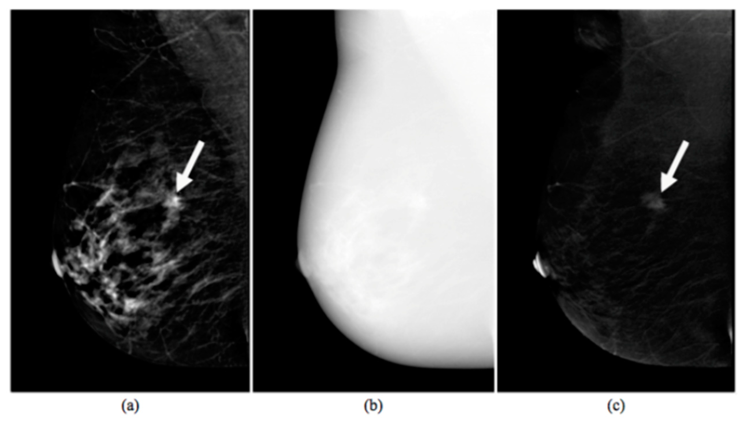
2.1.1. CESM Examination
2.1.2. Experimental Dataset
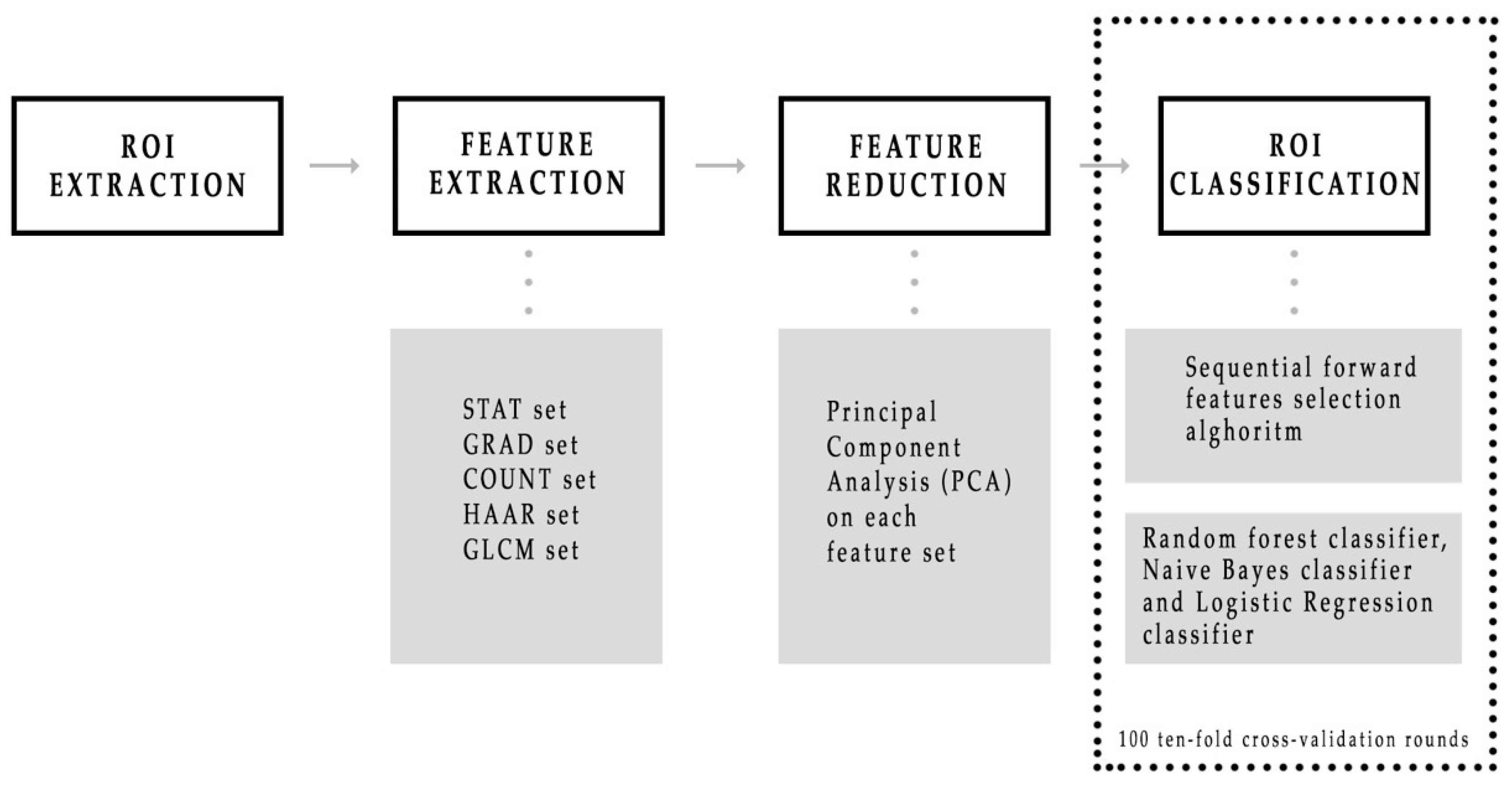
2.2. Methods
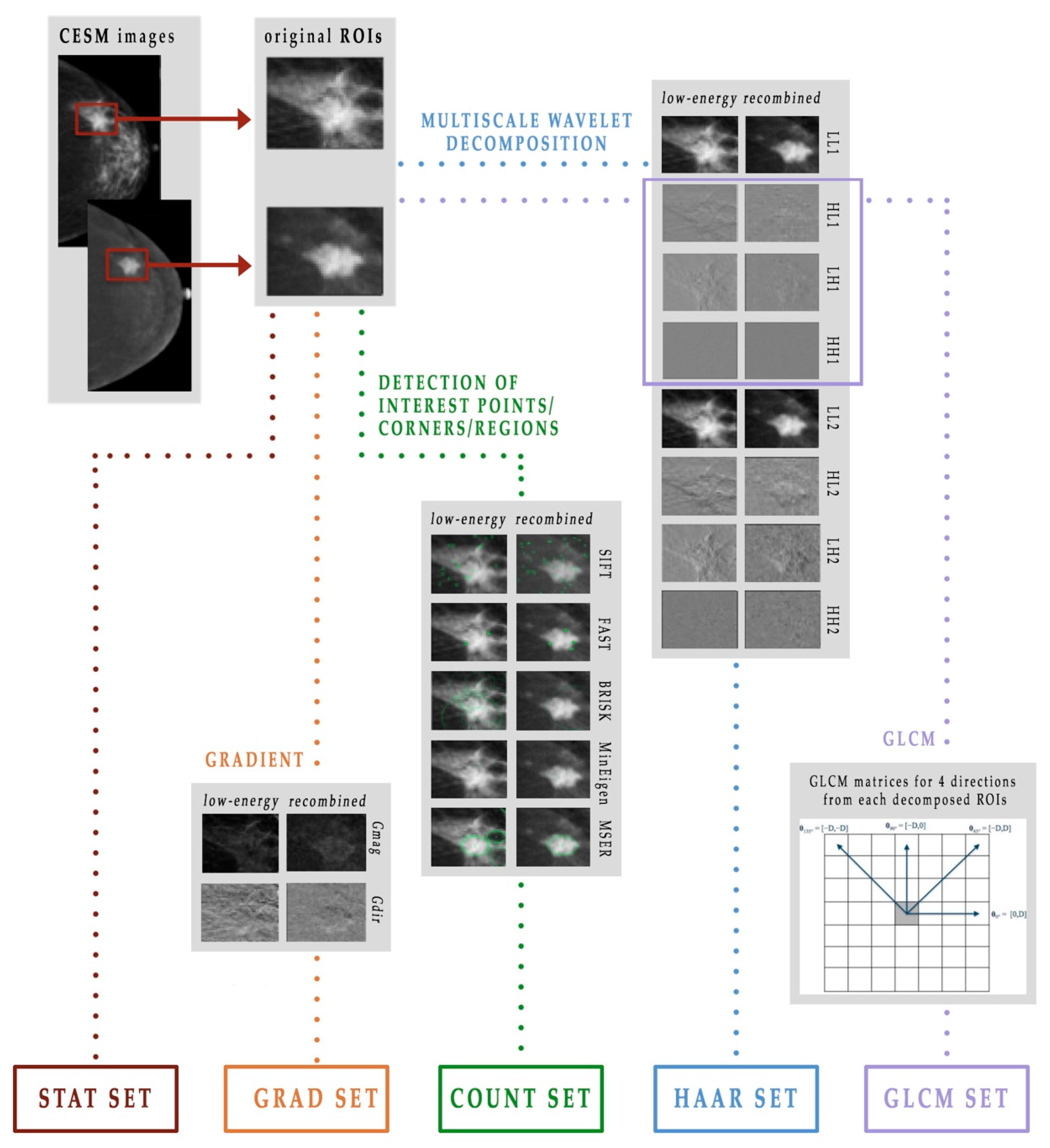
2.2.1. Feature Extraction
- Minimum eigenvalue algorithm, which underlies the Shi-Tomasi corner detection algorithm [32] for identifying the corners of an object
- Binary robust invariant scalable key-points (BRISK) method [35], which combines the SIFT and the FAST algorithms to feature detection, descriptor composition and key-points matching
- Maximally stable external regions (MSER) algorithm [36], which is a method of blob detection in images whose aim consists of finding correspondence between image elements from two images with different viewpoints.
2.2.2. Principal Component Analysis
2.2.3. Classification Model
3. Results
3.1. Principal Component Analysis
3.2. Classification Performances
4. Discussion
5. Conclusions
Author Contributions
Funding
Institutional Review Board Statement
Informed Consent Statement
Data Availability Statement
Conflicts of Interest
Abbreviations
| CC | Craniocaudal |
| CESM | Contrast-Enhanced Spectral Mammography |
| CI | Confidence Interval |
| CM | Contrast Medium |
| dir1 | Direction 1 (0_) |
| dir2 | Direction 2 (45_) |
| dir3 | Direction 3 (90_) |
| dir4 | Direction 4 (135_) |
| FN | False Negative |
| FP | False Positive |
| Gdir | Gradient direction |
| Gmag | Gradient magnitude |
| GLCM | Gray-Level Co-occurrence Matrix |
| HE | High Energy |
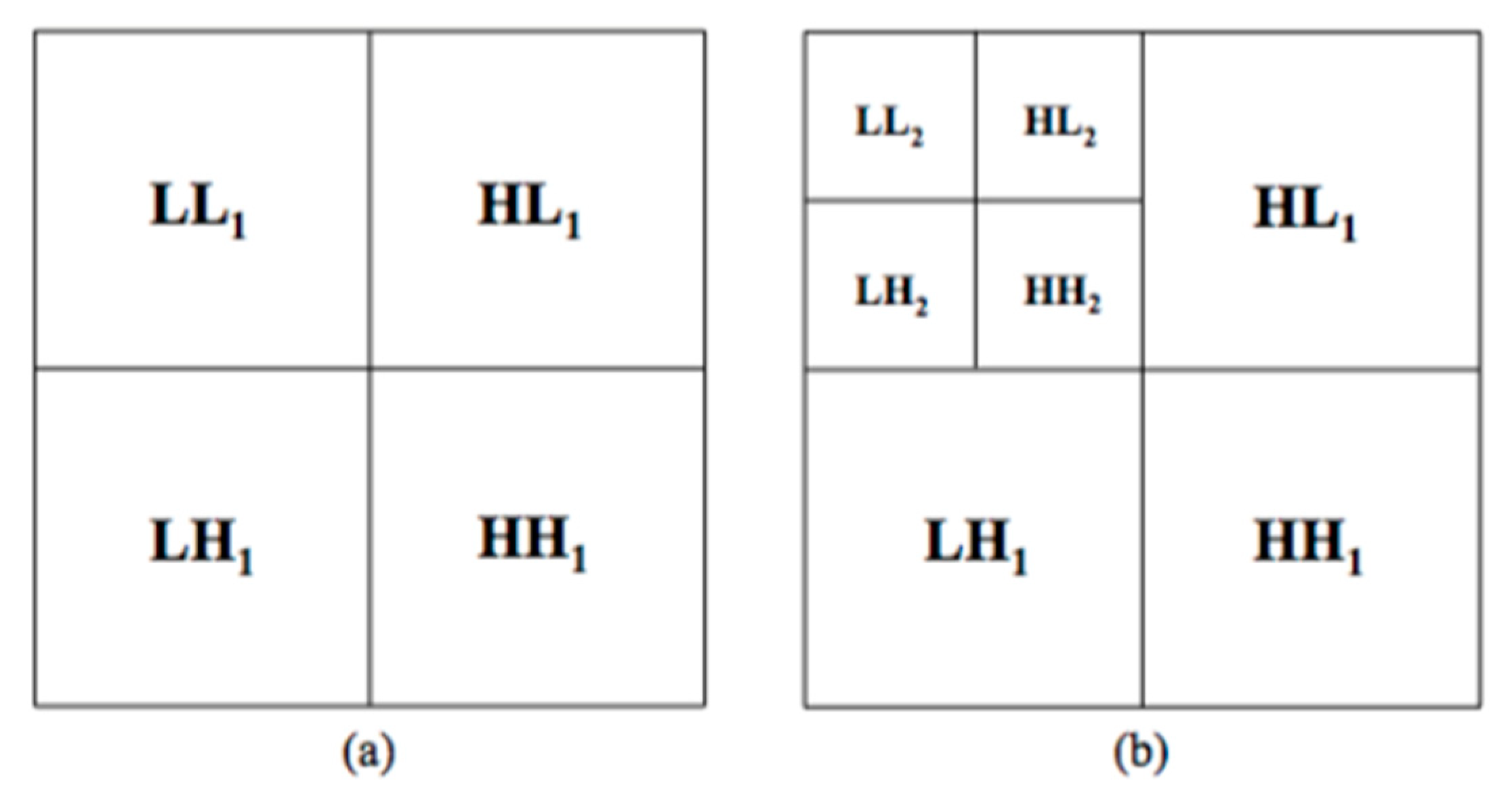
| HH | High-High |
| HL | High-Low |
| LDA | Linear Discriminant Analysis |
| LE | Low Energy |
| LH | Low-High |
| LL | Low-Low |
| MLO | Mediolateral Oblique |
| MR | Magnetic Resonance |
| PC(A) | Principal Component (Analysis) |
| RC | Recombined |
| RF | Random Forest |
| ROI | Region Of Interest |
| SD | Standard Deviation |
| TN | True Negative |
| TP | True Positive |
References
- Bray, F.; Ferlay, J.; Soerjomataram, I.; Siegel, R.L.; Torre, L.A.; Jemal, A. Global cancer statistics 2018: GLOBOCAN estimates of incidence and mortality worldwide for 36 cancers in 185 countries. CA Cancer J. Clin. 2018, 68, 394–424. [Google Scholar] [CrossRef] [PubMed]
- Cronin, K.A.; Lake, A.J.; Scott, S.; Sherman, R.L.; Noone, A.M.; Howlader, N.; Henley, S.J.; Anderson, R.N.; Firth, A.U.; Ma, J.; et al. Annual Report to the Nation on the Status of Cancer, part I: National cancer statistics. Cancer 2018, 124, 2785–2800. [Google Scholar] [CrossRef] [PubMed]
- Fallenberg, E.; Dromain, C.; Diekmann, F.; Engelken, F.; Krohn, M.; Singh, J.; Ingold-Heppner, B.; Winzer, K.; Bick, U.; Renz, D.M. Contrast-enhanced spectral mammography versus MRI: Initial results in the detection of breast cancer and assessment of tumor size. Eur. Radiol. 2014, 24, 256–264. [Google Scholar] [CrossRef] [PubMed]
- Tagliafico, A.S.; Mariscotti, G.; Valdora, F.; Durando, M.; Nori, J.; La Forgia, D.; Rosenberg, I.; Caumo, F.; Gandolfo, N.; Sormani, M.P.; et al. A prospective comparative trial of adjunct screening with tomosynthesis or ultrasound in women with mammography-negative dense breasts (ASTOUND-2). Eur. J. Cancer 2018, 104, 39–46. [Google Scholar] [CrossRef]
- Sardanelli, F.; Fallenberg, E.M.; Clauser, P.; Trimboli, R.M.; Camps-Herrero, J.; Helbich, T.H.; Forrai, G. Mammography: An update of the EUSOBI recommendations on information for women. Insights Imaging 2017, 8, 11–18. [Google Scholar] [CrossRef]
- Dilorenzo, G.; Telegrafo, M.; La Forgia, D.; Stabile Ianora, A.A.; Moschetta, M. Breast MRI background parenchymal enhanancement as imaging bridge to molecular cancer sub-type. Eur. J. Radiol. 2019, 113, 148–152. [Google Scholar] [CrossRef]
- Fausto, A.; Fanizzi, A.; Volterrani, L.; Mazzei, F.G.; Calabrese, C.; Casella, D.; Marcasciano, M.; Massafra, R.; La Forgia, D.; Mazzei, M.A. Feasibility, image quality and clinical evaluation of Contrast-Enhanced Breast MRI in supine position compared to standard prone position. Cancers 2020, 12, 2364. [Google Scholar] [CrossRef]
- Fausto, A.; Bernini, M.; La Forgia, D.; Fanizzi, A.; Marcasciano, M.; Volterrani, L.; Casella, D.; Mazzei, M.A. Six-year prospective evaluation of second-look US with volume navigation for MRI-detected additional breast lesions. Eur. Radiol. 2019, 29, 1799–1808. [Google Scholar] [CrossRef]
- Losurdo, L.; Basile, T.M.A.; Fanizzi, A.; Bellotti, R.; Bottigli, U.; Carbonara, R.; Dentamaro, R.; Diacono, D.; Didonna, V.; La Forgia, D.; et al. A Gradient-Based Approach for Breast DCE-MRI Analysis. Biomed. Res. Int. 2018, 16, 9032408. [Google Scholar] [CrossRef] [PubMed]
- Verma, B. Novel network architecture and learning algorithm for the classification of mass abnormalities in digitized mammograms. Artif. Intell. Med. 2008, 42, 67–79. [Google Scholar] [CrossRef] [PubMed]
- Rodríguez-Ruiz, A.; Krupinski, E.; Mordang, J.J.; Schilling, K.; Heywang-Köbrunner, S.H.; Sechopoulos, I.; Mann, R.M. Detection of breast cancer with mammography: Effect of an artificial intelligence support system. Radiology 2018, 290, 305–314. [Google Scholar] [CrossRef] [PubMed]
- Fanizzi, A.; Basile, T.M.; Losurdo, L.; Bellotti, R.; Bottigli, U.; Campobasso, F.; Didonna, V.; Fausto, A.; Massafra, R.; Tagliafico, A.; et al. Ensemble DiscreteWavelet Transform and Gray-Level Co-Occurrence Matrix for Microcalcification Cluster Classification in Digital Mammography. Appl. Sci. 2019, 9, 5388. [Google Scholar] [CrossRef]
- Fanizzi, A.; Basile, T.M.; Losurdo, L.; Bellotti, R.; Bottigli, U.; Dentamaro, R.; Didonna, V.; Fausto, A.; Massafra, R.; La Forgia, D.; et al. A Machine Learning Approach on Multiscale Texture Analysis for Breast Microcalcification Diagnosis. BMC Bioinform. 2020, 21 (Suppl. 2), 91. [Google Scholar] [CrossRef]
- Basile, T.M.A.; Fanizzi, A.; Losurdo, L.; Bellotti, R.; Bottigli, U.; Dentamaro, R.; Didonna, V.; Fausto, A.; Massafra, R.; La Forgia, D.; et al. Microcalcification Detection in Full-Field Digital Mammograms: A Fully Automated Computer-Aided System. Phys. Med. 2019, 64, 1–9. [Google Scholar] [CrossRef]
- Fanizzi, A.; Basile, T.M.A.; Losurdo, L.; Amoroso, N.; Bellotti, R.; Bottigli, U.; Dentamaro, R.; Didonna, V.; Fausto, A.; La Forgia, D.; et al. Hough transform for microcalcification detection in digital mammograms. Appl. Digit. Image Process. XL 2017, 10396, 41. [Google Scholar] [CrossRef]
- Dialani, V.; Slanetz, P.J.; Fein-Zachary, V.J.; Karimova, E.J.; Mehta, T.S.; Perry, H.; Phillips, J. Contrast-enhanced mammography: A systematic guide to interpretation and reporting. Am. Roentgen Ray Soc. 2019, 212, 222–231. [Google Scholar]
- Lalji, U.; Jeukens, C.; Houben, I.; Nelemans, P.; van Engen, R.; van Wylick, E.; Beets-Tan, R.; Wildberger, J.; Paulis, L.; Lobbes, M. Evaluation of low-energy contrast-enhanced spectral mammography images by comparing them to full-field digital mammography using EUREF image quality criteria. Eur. Radiol. 2015, 25, 2813–2820. [Google Scholar] [CrossRef]
- Del Mar Travieso-Aya, M.; Maldonado-Saluzzi, D.; Naranjo-Santana, P.; Fernandez Ruiz, C.; Severino-Rondon, W.; Rodriguez, M.; Vega Benitez, V.; Perez-Luzardo, O. Diagnostic performance of contrast-enhanced dual-energy spectral mammography (CESM): A retrospective study involving 644 breast lesions. La Radiol. Med. 2019, 124, 1006–1017. [Google Scholar] [CrossRef]
- Patel, B.K.; Ranjbar, S.; Wu, T.; Pockaj, B.A.; Li, J.; Zhang, N.; Lobbes, M.; Zhang, B.; Mitchell, J.R. Computer-aided diagnosis of contrast-enhanced spectral mammography: A feasibility study. Eur. J. Radiol. 2018, 98, 207–213. [Google Scholar] [CrossRef]
- Perek, S.; Kiryati, N.; Zimmerman-Moreno, G.; Sklair-Levy, M.; Konen, E.; Mayer, A. Classification of contrast-enhanced spectral mammography (CESM) images. Int. J. Comput. Assist. Radiol. Surg. 2018, 14, 1–9. [Google Scholar] [CrossRef]
- Fanizzi, A.; Losurdo, L.; Basile, T.; Bellotti, R.; Bottigli, U.; Delogu, P.; Diacono, D.; Didonna, V.; Fausto, A.; Lombardi, A.; et al. Fully automated support system for diagnosis of breast cancer in contrast-enhanced spectral mammography images. J. Clin. Med. 2019, 8, 891. [Google Scholar] [CrossRef]
- La Forgia, D.; Fanizzi, A.; Campobasso, F.; Bellotti, R.; Didonna, V.; Lorusso, V.; Moschetta, M.; Massafra, R.; Tamborra, P.; Tangaro, S.; et al. Radiomic Analysis in Contrast-Enhanced Spectral Mammography for Predicting Breast Cancer Histological Outcome. Diagnostics 2020, 10, 708. [Google Scholar] [CrossRef]
- Losurdo, L.; Fanizzi, A.; Basile, T.M.A.; Bellotti, R.; Bottigli, U.; Dentamaro, R.; Didonna, V.; Lorusso, V.; Massafra, R.; Tamborra, P.; et al. Radiomics Analysis on Contrast-Enhanced Spectral Mammography Images for Breast Cancer Diagnosis:A Pilot Study. Entropy 2019, 21, 1110. [Google Scholar] [CrossRef]
- Wang, Z.; Lin, F.; Ma, H.; Shi, Y.; Dong, J.; Yang, P.; Zhang, K.; Guo, N.; Zhang, R.; Cui, J.; et al. Contrast-Enhanced Spectral Mammography-Based Radiomics Nomogram for the Prediction of Neoadjuvant Chemotherapy-Insensitive Breast Cancers. Front. Oncol. 2021, 11, 605230. [Google Scholar] [CrossRef]
- Iotti, V.; Ravaioli, S.; Vacondio, R.; Coriani, C.; Caffarri, S.; Sghedoni, R.; Nitrosi, A.; Ragazzi, M.; Gasparini, E.; Masini, C.; et al. Contrast-enhanced spectral mammography in neoadjuvant chemotherapy monitoring: A comparison with breast magnetic resonance imaging. Breast Cancer Res. 2017, 19, 106. [Google Scholar] [CrossRef] [PubMed]
- Saeys, Y.; Inza, I.; Larrañaga, P. A review of feature selection techniques in bioinformatics. Bioinformatics 2007, 23, 2507–2517. [Google Scholar] [CrossRef]
- D’Orsi, C.; Sickles, E.; Mendelson, E.; Morris, E. 2013 ACR BI-RADS Atlas: Breast Imaging Reporting and Data System; American College of Radiology: Reston, VA, USA, 2014. [Google Scholar]
- Woods, R.; Gonzales, R. Digital Image Processing, 2nd ed.; Prentice Hall: Hoboken, NJ, USA, 2002. [Google Scholar]
- Gupta, P.; Kumar, V. Importance of statistical measures in digital image processing. Int. J. Emerg. Technol. Adv. Eng. 2012, 2, 56–62. [Google Scholar]
- Lowe, D.G. Object recognition from local scale-invariant features. In Proceedings of the Seventh IEEE International Conference on Computer Vision, Corfu, Greece, 20–25 September 1999; IEEE Computer Society: Washington, DC, USA, 1999; Volume 2, pp. 1150–1157. [Google Scholar]
- Lindeberg, T. Scale invariant feature transform. Scholarpedia 2012, 7, 10491. [Google Scholar] [CrossRef]
- Shi, J.; Tomasi, C. Good features to track. In Proceedings of the Ninth IEEE Conference on Computer Vision and Pattern Recognition, Seattle, WA, USA, 21–23 June 1994; pp. 593–600. [Google Scholar]
- Rosten, E.; Drummond, T. Fusing points and lines for high performance tracking. In Proceedings of the Tenth IEEE International Conference on Computer Vision, Beijing, China, 17–20 October 2005; pp. 1508–1515. [Google Scholar]
- Rosten, E.; Drummond, T. Machine learning for high-speed corner detection. In European Conference on Computer Vision; Springer: Berlin/Heidelberg, Germany, 2006; Volume 3951, pp. 430–443. [Google Scholar]
- Leutenegger, S.; Chli, M.; Siegwart, R.Y. BRISK: Binary robust invariant scalable keypoints. In Proceedings of the 2011 IEEE International Conference on Computer Vision (ICCV), Barcelona, Spain, 6–13 November 2011; pp. 2548–2555. [Google Scholar]
- Matas, J.; Chum, O.; Urban, M.; Pajdla, T. Robust wide-baseline stereo from maximally stable extremal regions. Image Vis. Comput. 2004, 22, 761–767. [Google Scholar] [CrossRef]
- Mallat, S.G. A theory for multiresolution signal decomposition: The wavelet representation. IEEE Trans. Pattern Anal. Mach. Intell. 1989, 11, 674–693. [Google Scholar] [CrossRef]
- Haralick, R.M.; Shanmugam, K. Textural features for image classification. IEEE Trans. Syst. Man Cybern. 1973, 6, 610–621. [Google Scholar] [CrossRef]
- Mohanaiah, P.; Sathyanarayana, P.; GuruKumar, L. Image texture feature extraction using GLCM approach. Int. J. Sci. Res. Publ. 2013, 3, 1. [Google Scholar]
- Jolliffe, I. Principal Component Analysis; Springer: Cham, Switzerland, 2011. [Google Scholar]
- Breiman, L. Random forests. Mach. Learn. 2001, 45, 5–32. [Google Scholar] [CrossRef]
- Webb, G.I.; Bayes, N. Encyclopedia of Machine Learning and Data Mining; Springer: Berlin/Heidelberg, Germany, 2017. [Google Scholar]
- Rymarczyk, T.; Kozłowski, E.; Kłosowski, G.; Niderla, K. Logistic Regression for Machine Learning in Process Tomography. Sensors 2019, 19, 3400. [Google Scholar] [CrossRef] [PubMed]
- Aha, D.W.; Bankert, R.L. A comparative evaluation of sequential feature selection algorithms. In Learning from Data; Springer: Berlin, Germany, 1996; pp. 199–206. [Google Scholar]
- Hastie, T.; Tibshirani, R.; Friedman, J.; Franklin, J. The elements of statistical learning: Data mining, inference and prediction. Math. Intell. 2005, 27, 83–85. [Google Scholar]
- Youden, W. Index for rating diagnostic tests. Cancer 1950, 3, 32–35. [Google Scholar] [CrossRef]


| PCs’ Set | Classifier | PCs Best Combination | AUC (%) | Acc (%) | Sens (%) | Spec (%) |
|---|---|---|---|---|---|---|
| STAT | RF | 1 + 2 | 78.29 | 77.59 | 81.40 | 73.33 |
| NB | 1 | 81.71 | 74.14 | 67.44 | 93.33 | |
| GLM | 1 | 83.49 | 74.41 | 67.44 | 93.33 | |
| GRAD | RF | 1 + 5 | 85.31 | 81.03 | 79.07 | 93.33 |
| NB | 1 + 2 | 76.59 | 75.86 | 76.74 | 73.33 | |
| GLM | 1 + 5 + 2 + 9 | 83.10 | 74.14 | 65.12 | 100 | |
| COUNT | RF | 1 + 3 | 66.82 | 62.07 | 58.14 | 0.8 |
| NB | 2 + 1 | 64.88 | 60.34 | 50.00 | 86.67 | |
| GLM | 1 + 3 | 75.66 | 79.31 | 88.37 | 53.33 | |
| HAAR | RF | 2 + 12 | 94.65 | 87.93 | 86.05 | 100 |
| NB | 1 + 3 + 16 + 19 + 15 + 14 | 86.51 | 84.48 | 87.21 | 80.00 | |
| GLM | 1 + 3 + 9 + 19 + 16 + 8 + 12 | 83.72 | 77.59 | 74.42 | 93.33 | |
| GLCM | RF | 2 + 1 | 86.40 | 81.03 | 79.07 | 86.67 |
| NB | 2 + 4 + 1 + 11 + 10 + 9 | 75.50 | 75.86 | 72.09 | 86.67 | |
| GLM | 2 + 4 + 1 + 9 + 11 + 10 | 82.33 | 87.93 | 93.02 | 73.33 |
| Set | PC | Important Features | ||||
|---|---|---|---|---|---|---|
| STAT | 1 | RC_Entropy | RC_Std | RC_Max-Min | RC_Relative Smoothness | RC_ Variance |
| GRAD | 1 | RC_Mean_ Gmag | LE_Mean_ Gmag | RC_Entropy_ Gmag | RC_Relative Smoothness_Gmag | RC_Variance_ Gmag |
| 5 | LE_Kurtosis_ Gmag | LE_Skewness_ Gdir | RC_Skewness_ Gdir | RC_Kurtosis_ Gdir | RC_Entropy_ Gdir | |
| COUNT | 1 | RC_Fast | RC_Brisk | LE_Brisk | LE_Fast | |
| 3 | LE_Sift | RC_Sift | LE_MSER | RC_Minimum Eigenvalue | ||
| HAAR | 2 | LE_Relative Smoothness_ HL2 | LE_ Relative Smoothness_ LH2 | LE_ Relative Smoothness_ HL1 | LE_Entropy_ LL1 | LE_Relative Smoothness_ HH2 |
| 12 | LE_Skewnes_ LL1 | RC_Skewness_ LH2 | LE_Kurtosis_ HL1 | LE_Skewness_ HH1 | ||
| GLCM | 2 | RC_Sum Entropy_ HH1 dir2 | RC_Entropy_ HH1 dir2 | RC_Entropy_ HH1 dir3 | RC_Entropy_ HH1 dir4 | RC_Sum Entropy_ HH1 dir4 |
| 1 | LE_Sum Average_ HH1 dir3 | LE_Sum Average_ HH1 dir1 | LE_Sum Average_ HH1 dir4 | LE_Sum Average_ HH1 dir2 | ||
| Classifier | Best Model | AUC (%) | Acc (%) | Sens (%) | Spec (%) |
|---|---|---|---|---|---|
| RF | H2 + G1 + H12 | 95.66 | 90.52 | 88.37 | 100 |
| NB | S1 + GL10 + G2 + GL11 + H16 + H3 + H19 | 88.99 | 89.66 | 93.02 | 80 |
| GLM | S1 + G2 + G9 + S3 + H8 + GL2 + GL1 | 90.08 | 84.48 | 81.40 | 100 |
| Article | No. of ROIs | Features | Classifier | Performance (%) |
|---|---|---|---|---|
| Patel et al. [19] | 50 | SVM | AUC: 95 Acc: 90 Sens: 88 Spec: 92 | |
| Perek et al. [20] | 129 | Multimodal Network | AUC: 89 Sens: 100 Spec: 66 | |
| Fanizzi et al. [21] | 48 | 12 | Random Forest | AUC: 93.1 Acc: 87.5 Sens: 87.5 Spec: 91.7 |
| Losurdo et al. [23] | 55 | 10 | SVM | Acc: 80.91 Sens: 90.28 Spec: 71.55 |
| Best proposed model | 58 | 2 | Random Forest | AUC: 95.66 Acc: 90.52 Sens: 88.37 Spec: 100 |
Publisher’s Note: MDPI stays neutral with regard to jurisdictional claims in published maps and institutional affiliations. |
© 2021 by the authors. Licensee MDPI, Basel, Switzerland. This article is an open access article distributed under the terms and conditions of the Creative Commons Attribution (CC BY) license (https://creativecommons.org/licenses/by/4.0/).
Share and Cite
Massafra, R.; Bove, S.; Lorusso, V.; Biafora, A.; Comes, M.C.; Didonna, V.; Diotaiuti, S.; Fanizzi, A.; Nardone, A.; Nolasco, A.; et al. Radiomic Feature Reduction Approach to Predict Breast Cancer by Contrast-Enhanced Spectral Mammography Images. Diagnostics 2021, 11, 684. https://doi.org/10.3390/diagnostics11040684
Massafra R, Bove S, Lorusso V, Biafora A, Comes MC, Didonna V, Diotaiuti S, Fanizzi A, Nardone A, Nolasco A, et al. Radiomic Feature Reduction Approach to Predict Breast Cancer by Contrast-Enhanced Spectral Mammography Images. Diagnostics. 2021; 11(4):684. https://doi.org/10.3390/diagnostics11040684
Chicago/Turabian StyleMassafra, Raffaella, Samantha Bove, Vito Lorusso, Albino Biafora, Maria Colomba Comes, Vittorio Didonna, Sergio Diotaiuti, Annarita Fanizzi, Annalisa Nardone, Angelo Nolasco, and et al. 2021. "Radiomic Feature Reduction Approach to Predict Breast Cancer by Contrast-Enhanced Spectral Mammography Images" Diagnostics 11, no. 4: 684. https://doi.org/10.3390/diagnostics11040684
APA StyleMassafra, R., Bove, S., Lorusso, V., Biafora, A., Comes, M. C., Didonna, V., Diotaiuti, S., Fanizzi, A., Nardone, A., Nolasco, A., Ressa, C. M., Tamborra, P., Terenzio, A., & La Forgia, D. (2021). Radiomic Feature Reduction Approach to Predict Breast Cancer by Contrast-Enhanced Spectral Mammography Images. Diagnostics, 11(4), 684. https://doi.org/10.3390/diagnostics11040684