
Impact of Radiation Quality on Microdosimetry and Chromosome Aberrations for High-Energy (>250 MeV/n) Ions


Abstract
:1. Introduction
2. Materials and Methods
2.1. Macro-Scale Approach
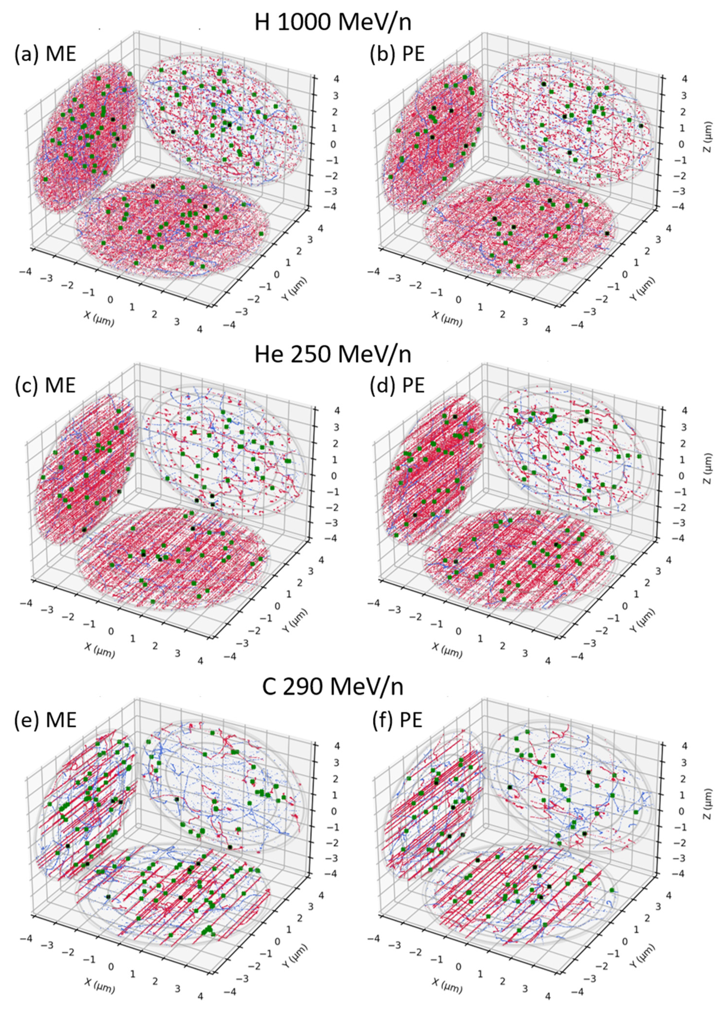
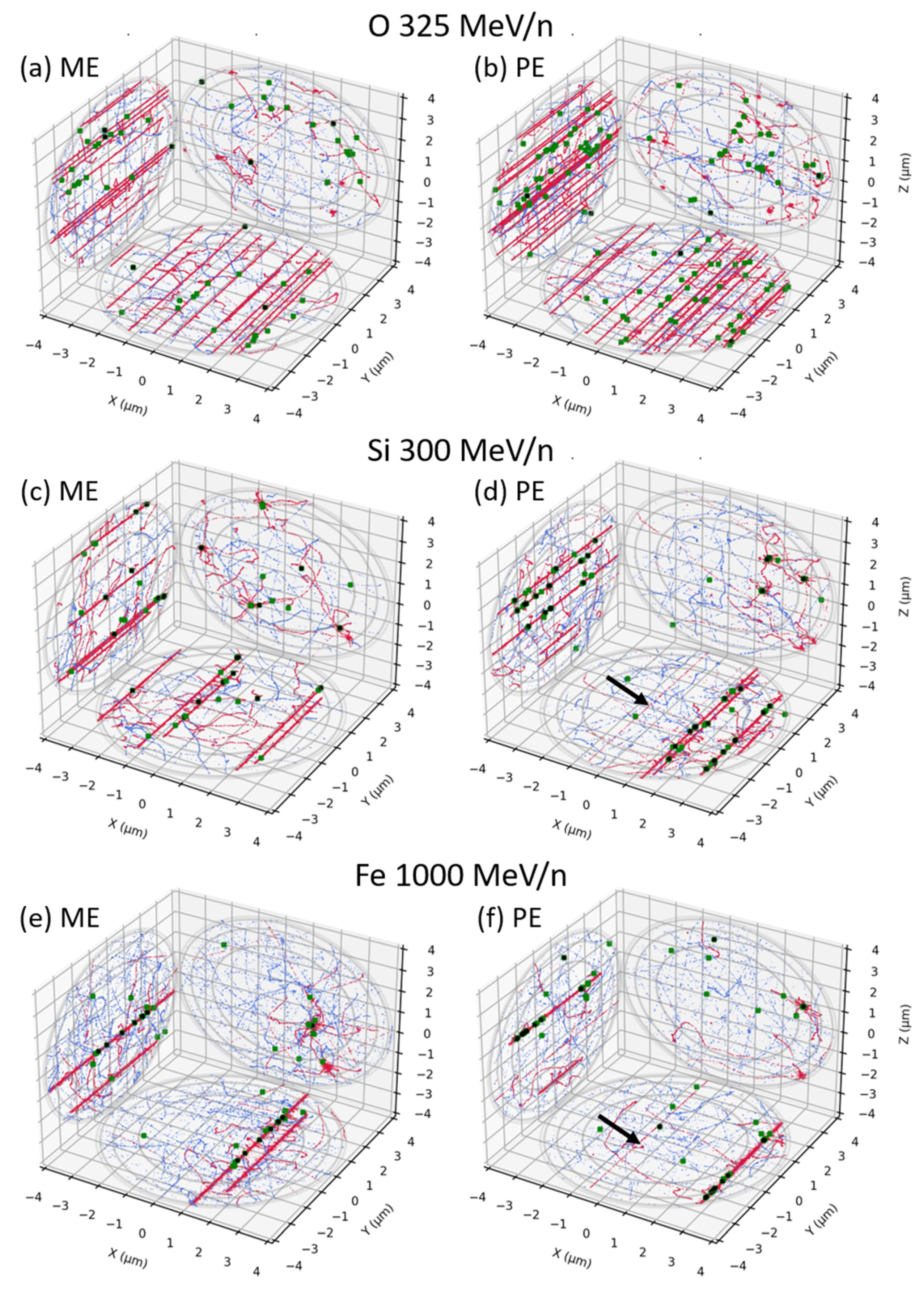
2.2. Micro-Scale Approach
3. Results and Discussion
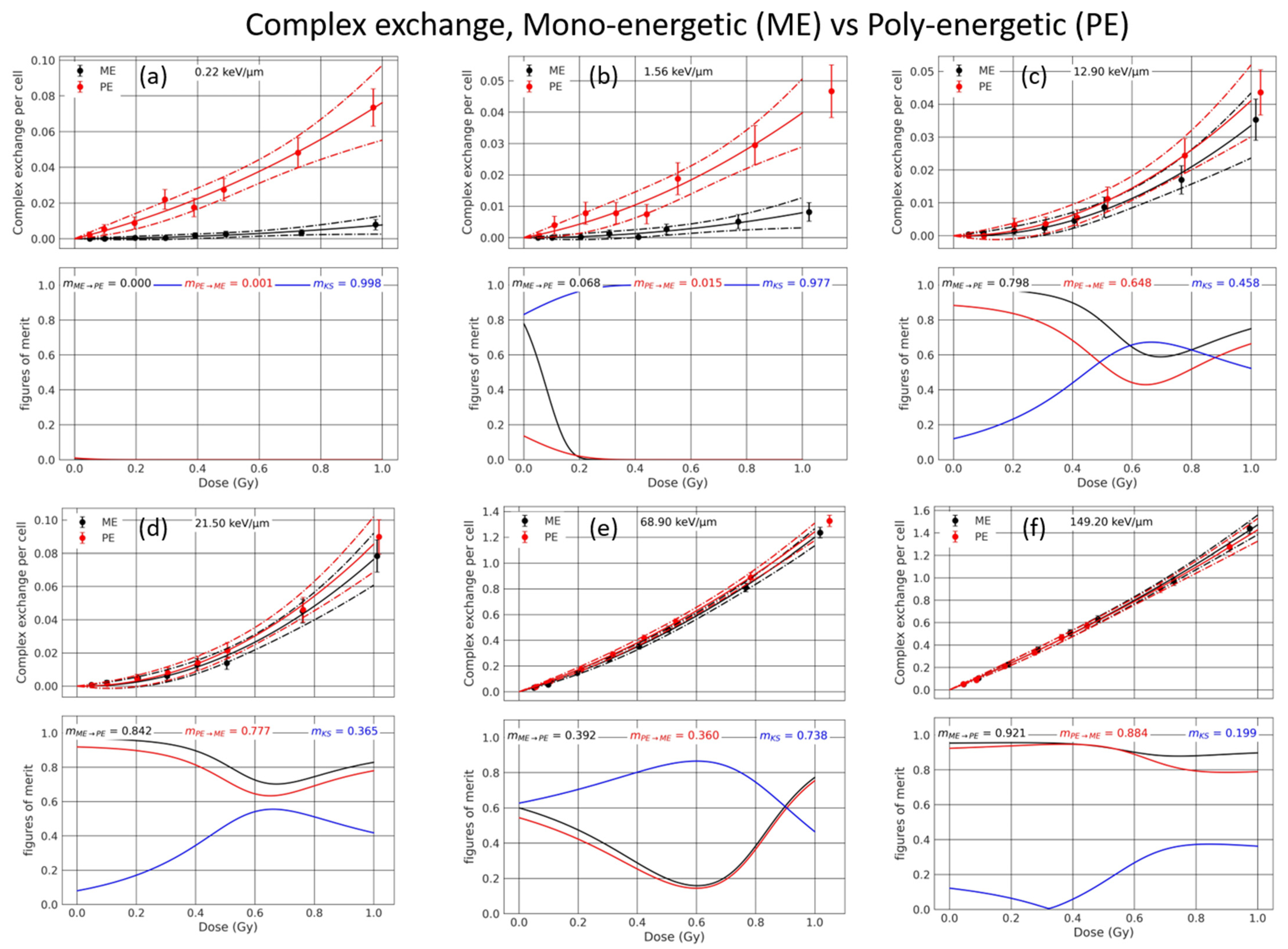
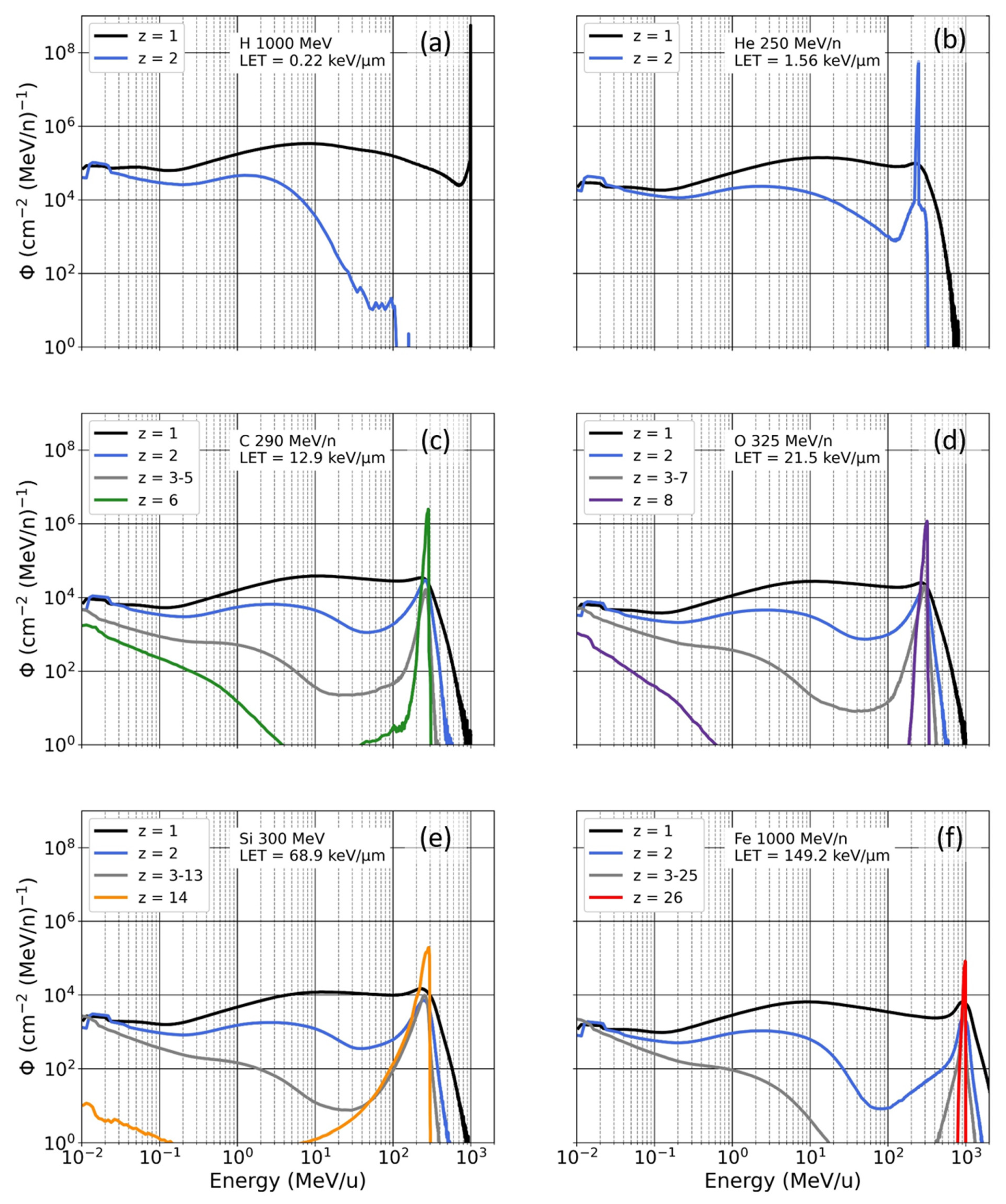
3.1. Mono-Energetic Beam vs. Poly-Energetic Spectra
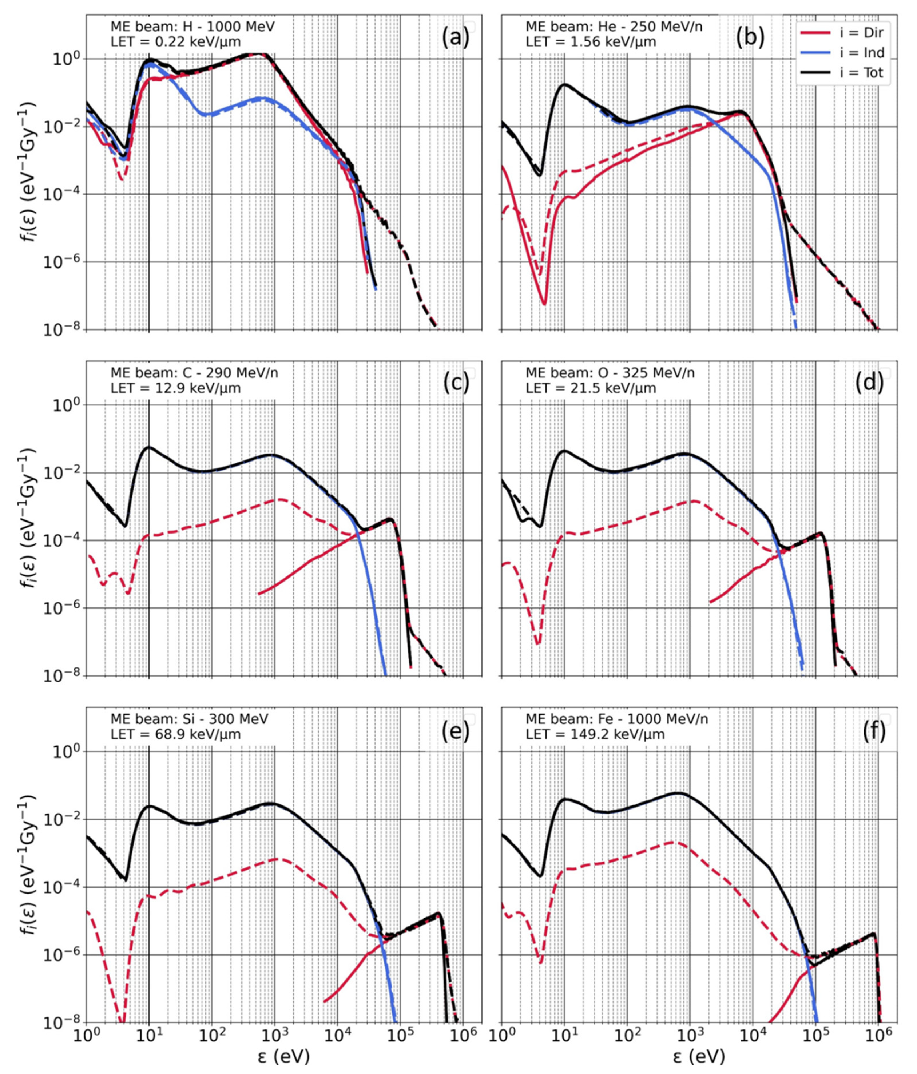
3.2. Microdosimetry
3.3. Chromosome Aberrations
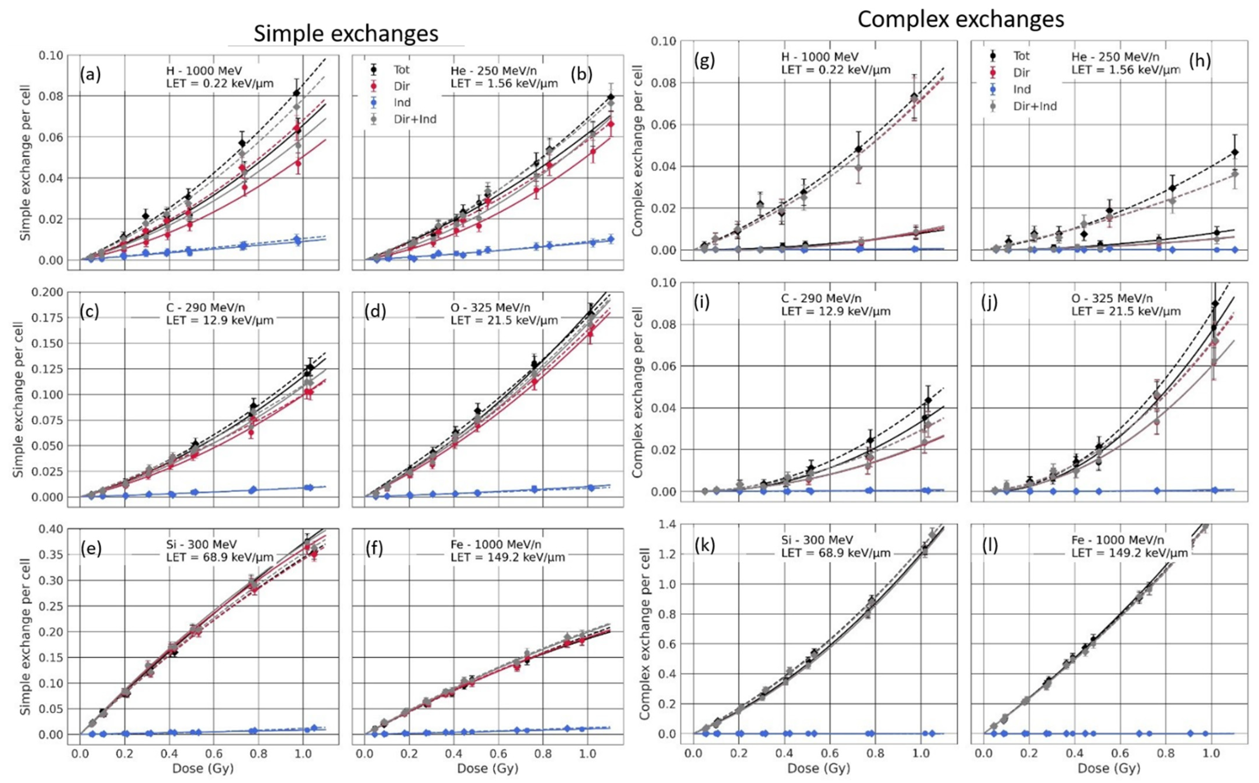
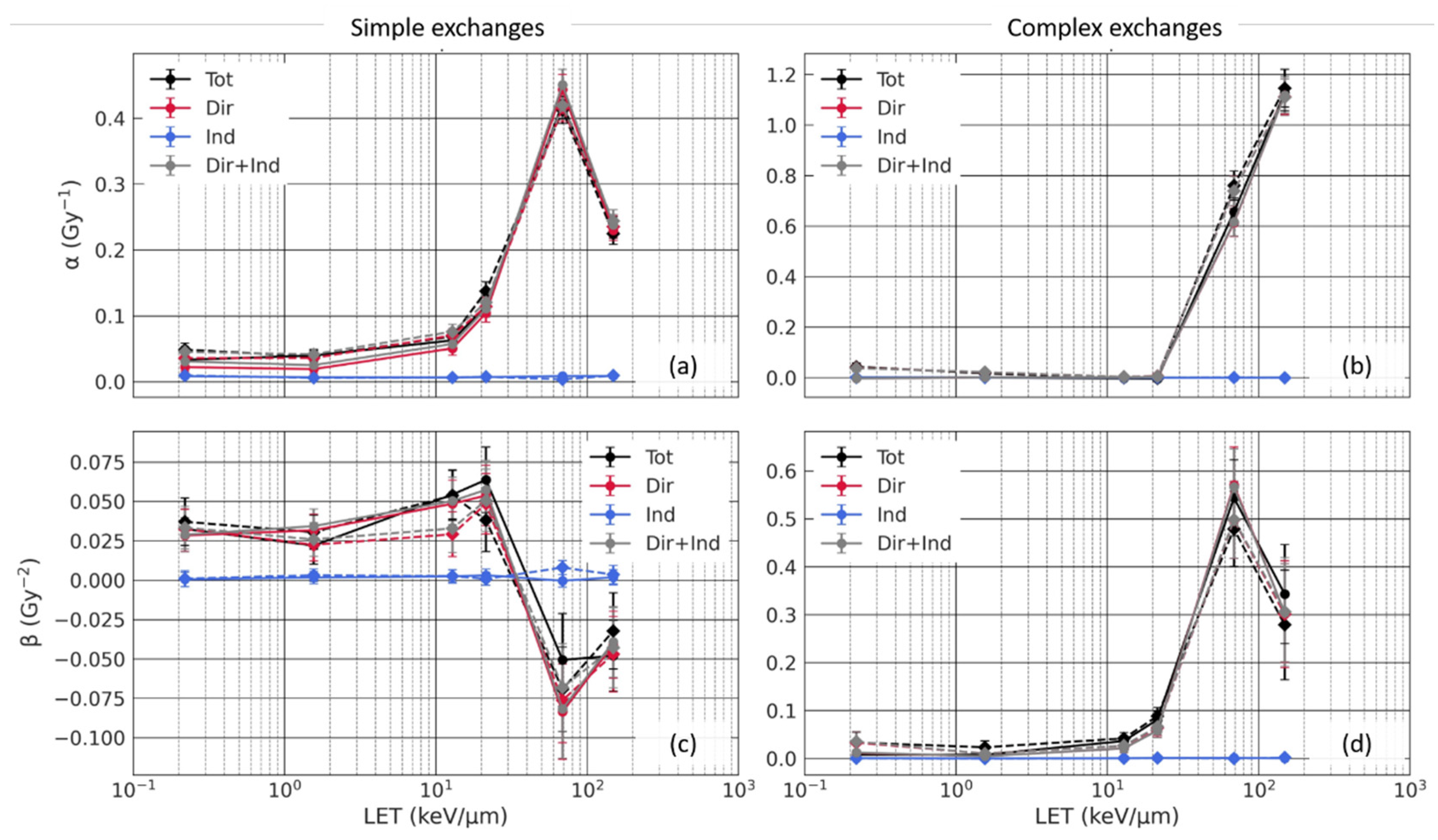
3.3.1. Analysis of the Sub-Contributions for Mono-Energetic Beams
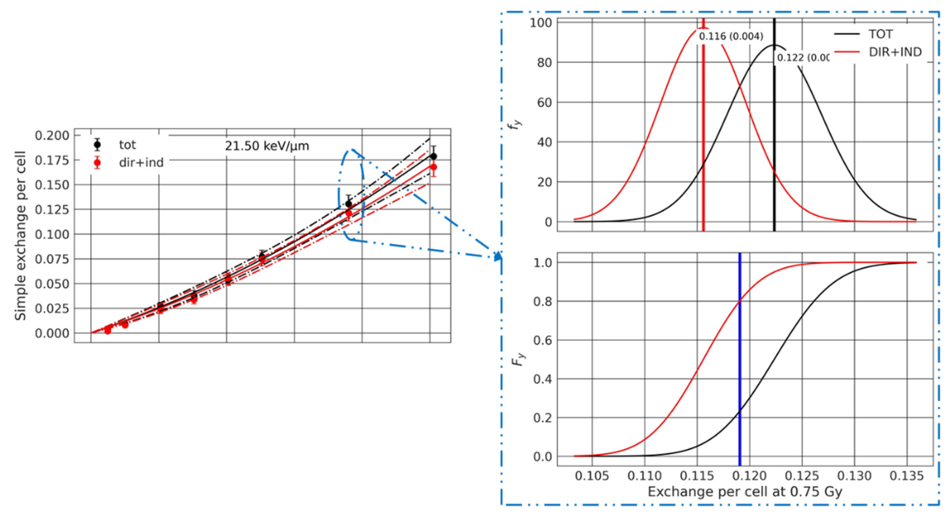
3.3.2. Analysis of the Effect of Beam Transport
4. Conclusions
Author Contributions
Funding
Institutional Review Board Statement
Informed Consent Statement
Data Availability Statement
Conflicts of Interest
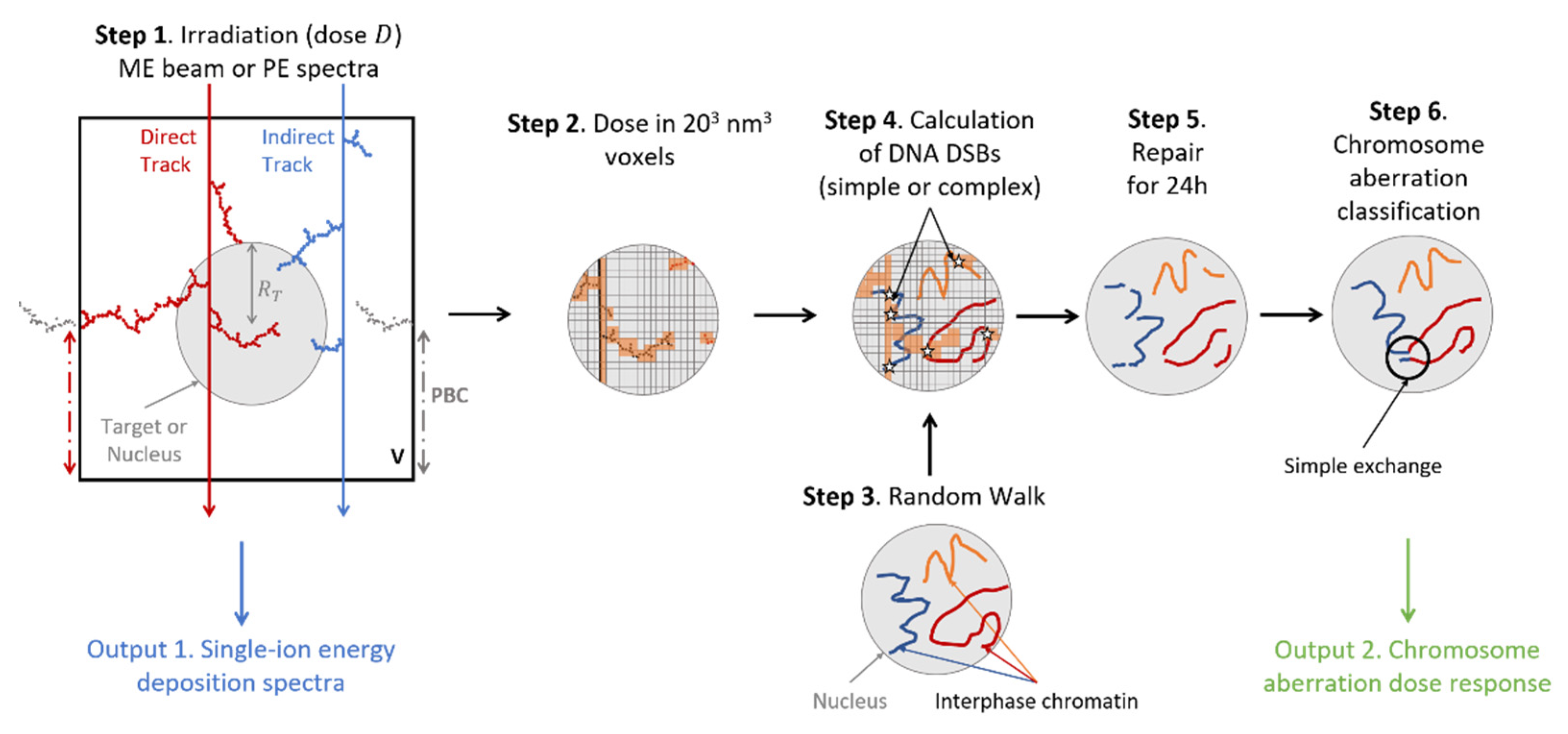
Appendix A. RITRACKS/RITCARD Simulation
Appendix A.1. Simulation of Micrometric Volume Irradiation
Appendix A.2. Single-Ion Energy Deposition Spectra
Appendix A.3. Chromosome Aberrations
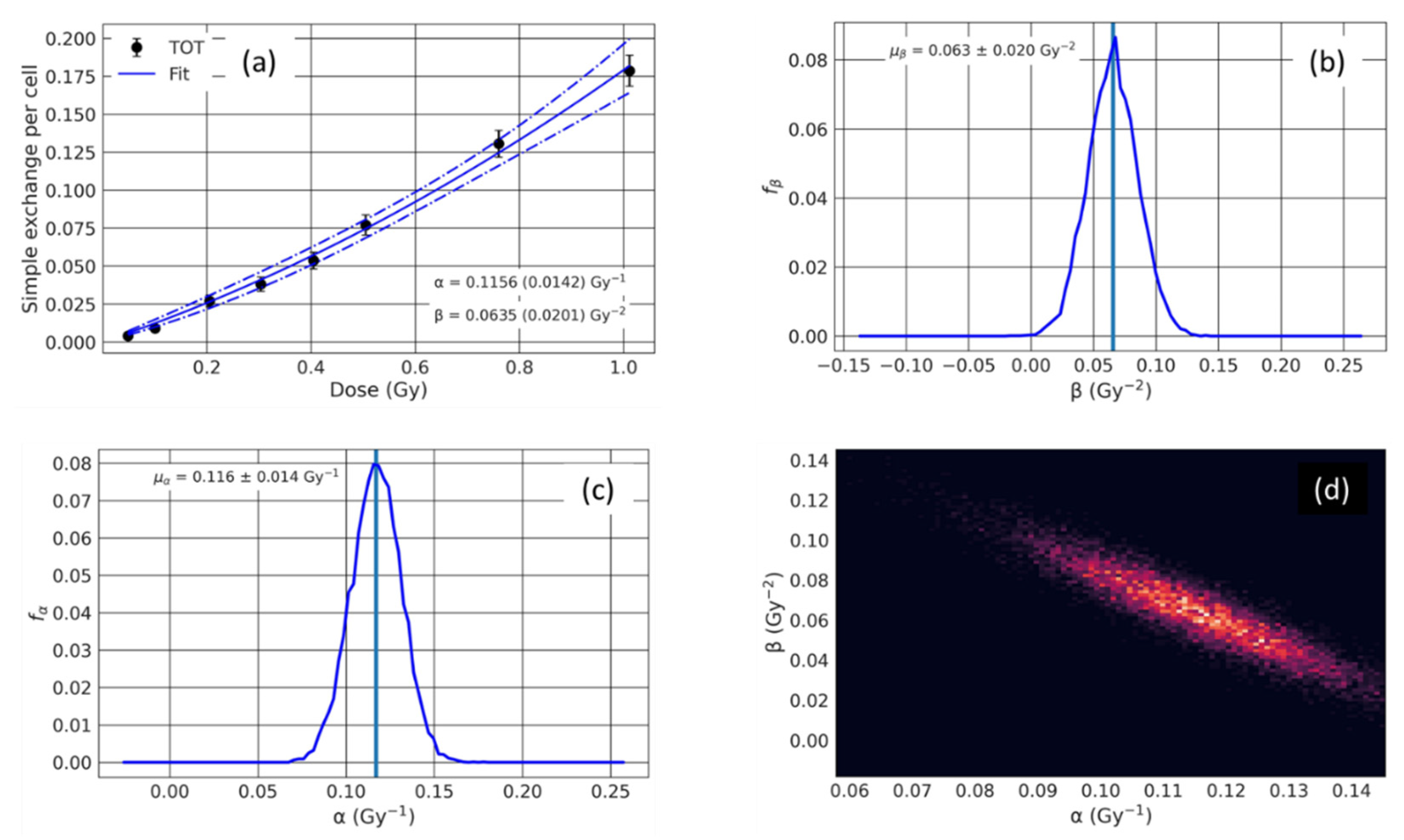
Appendix A.4. Dose–Response Statistical Analysis


References
- Simonsen, L.C.; Slaba, T.C.; Guida, P.; Rusek, A. NASA’s first ground-based Galactic Cosmic Ray Simulator: Enabling a new era in space radiobiology research. PLoS Biol. 2020, 18, e3000669. [Google Scholar] [CrossRef]
- Durante, M.; Cucinotta, F.A. Heavy ion carcinogenesis and human space exploration. Nat. Rev. Cancer 2008, 8.6, 465–472. [Google Scholar] [CrossRef] [PubMed]
- Bonassi, S.; Norppa, H.; Ceppi, M.; Strömberg, U.; Vermeulen, R.; Znaor, A.; Cebulska-Wasilewska, A.; Fabianova, E.; Fucic, A.; Gundy, S.; et al. Chromosomal aberration frequency in lymphocytes predicts the risk of cancer: Results from a pooled cohort study of 22 358 subjects in 11 countries. Carcinog. 2008, 29, 1178–1183. [Google Scholar] [CrossRef] [PubMed] [Green Version]
- Sridharan, D.M.; Asaithamby, A.; Blattnig, S.R.; Costes, S.V.; Doetsch, P.W.; Dynan, W.S.; Hahnfeldt, P.; Hlatky, L.; Kidane, Y.; Kronenberg, A.; et al. Evaluating biomarkers to model cancer risk post cosmic ray exposure. Life Sci. Space Res. 2016, 9, 19–47. [Google Scholar] [CrossRef] [PubMed] [Green Version]
- Rossi, H.; Zaider, M. Microdosimetry and Its Applications; John Libbey: Montrouge, France, 1996; pp. 205–278. [Google Scholar]
- Plante, I.; Poignant, F.; Slaba, T. Track Structure Components: Characterizing Energy Deposited in Spherical Cells from Direct and Peripheral HZE Ion Hits. Life 2021, 11, 1112. [Google Scholar] [CrossRef] [PubMed]
- Plante, I.; Cucinotta, F.A. Monte-Carlo Simulation of Ionizing Radiation Tracks. In Monte-Carlo Simulation of Ionizing Radiation tracks in Applications of Monte Carlo Methods in Biology, Medicine and Other Fields of Science; Mode, C.B., Ed.; InTechOpen: London, UK, 2011; pp. 315–356. [Google Scholar] [CrossRef] [Green Version]
- Dogdas, B.; Stout, D.; Chatziioannou, A.F.; Leahy, R.M. Digimouse: A 3D whole body mouse atlas from CT and cryosection data. Phys. Med. Biol. 2007, 52, 577. [Google Scholar] [CrossRef] [PubMed] [Green Version]
- Agostinelli, S.; Allison, J.; Amako, K.A.; Apostolakis, J.; Araujo, H.; Arce, P.; Asai, M.; Axen, D.; Banerjee, S.; Barrand, G.J.N.I.; et al. GEANT4—A simulation toolkit. Nucl. Instrum. Methods Phys. Res. A. 2003, 506, 250–303. [Google Scholar] [CrossRef] [Green Version]
- Plante, I.; Ponomarev, A.; Patel, Z.; Slaba, T.; Hada, M. RITCARD: Radiation-Induced Tracks, Chromosome Aberrations, Repair and Damage. Radiat. Res. 2019, 192, 282–298. [Google Scholar] [CrossRef]
- Suman, S.; Kumar, S.; Moon, B.-H.; Fornace, A.J.; Datta, K. Low and high dose rate heavy ion radiation-induced intestinal and colonic tumorigenesis in APC1638N/+ mice. Life Sci. Space Res. 2017, 13, 45–50. [Google Scholar] [CrossRef]
- Shuryak, I.; Slaba, T.C.; Plante, I.; Poignant, F.; Blattnig, S.T.; Brenner, D.J. A Practical Approach for Continuous In-Situ characterization of radiation quality factors in space. Sci. Rep. 2022, 12, 1–10. [Google Scholar] [CrossRef]
- Plante, I.; Slaba, T.C.; Shavers, Z.; Hada, M. A bi-exponential repair algorithm for radiation-induced double-strand breaks: Application to simulation of chromosome aberrations. Genes 2019, 10, 936. [Google Scholar] [CrossRef] [PubMed] [Green Version]
- Slaba, T.C.; Plante, I.; Ponomarev, A.; Patel, Z.S.; Hada, M. Determination of chromosome aberrations in human fibroblasts irradiated by mixed fields generated with shielding. Radiat. Res. 2020, 194, 246–258. [Google Scholar] [CrossRef] [PubMed]
- Pariset, E.; Plante, I.; Ponomarev, A.; Viger, L.; Evain, T.; Blattnig, S.R.; Costes, S.V. DNA break clustering inside repair domains predicts cell death and mutation frequency in human fibroblasts and in Chinese hamster cells for a 10^ 3× range of linear energy transfers. Biorxiv 2020. [Google Scholar] [CrossRef]
- Hada, M.; Sutherland, B.M. Spectrum of complex DNA damages depends on the incident radiation. Radiat. Res. 2006, 165, 223–230. [Google Scholar] [CrossRef]
- Asaithamby, A.; Uematsu, N.; Chatterjee, A.; Story, M.D.; Burma, S.; Chen, D.J. Repair of HZE-particle-induced DNA double-strand breaks in normal human fibroblasts. Radiat. Res. 2008, 169, 437–446. [Google Scholar] [CrossRef] [PubMed]
- Ham, D.W.; Song, B.; Gao, J.; Yu, J.; Sachs, R.K. Synergy theory in radiobiology. Radiat. Res. 2018, 189, 225–237. [Google Scholar] [CrossRef]
- Huang, E.G.; Lin, Y.; Ebert, M.; Ham, D.W.; Zhang, C.Y.; Sachs, R.K. Synergy theory for murine Harderian gland tumours after irradiation by mixtures of high-energy ionized atomic nuclei. Radiat. Environ. Biophys. 2019, 58, 151–166. [Google Scholar] [CrossRef] [Green Version]
- Huang, E.G.; Wang, R.-Y.; Xie, L.; Chang, P.; Yao, G.; Zhang, B.; Ham, D.W.; Lin, Y.; Blakely, E.A.; Sachs, R.K. Simulating galactic cosmic ray effects: Synergy modeling of murine tumor prevalence after exposure to two one-ion beams in rapid sequence. Life Sci. Space Res. 2020, 25, 107–118. [Google Scholar] [CrossRef]
- George, K.A.; Hada, M.; Chappell, L.; Cucinotta, F.A. Biological effectiveness of accelerated particles for the induction of chromosome damage: Track structure effects. Radiat. Res. 2013, 180, 25–33. [Google Scholar] [CrossRef]
- George, K.A.; Hada, M.; Cucinotta, F.A. Biological effectiveness of accelerated protons for chromosome exchanges. Front. Oncology 2015, 5, 226. [Google Scholar] [CrossRef] [Green Version]
- George, K.; Durante, M.; Wu, H.; Willingham, V.; Cucinotta, F.A. In vivo and in vitro measurements of complex-type chromosomal exchanges induced by heavy ions. Adv. Space Res. 31 2003, 6, 1525–1535. [Google Scholar] [CrossRef]
- George, K.; Durante, M.; Willingham, V.; Wu, H.; Yang, T.C.; Cucinotta, F.A. Biological effectiveness of accelerated particles for the induction of chromosome damage measured in metaphase and interphase human lymphocytes. Radiat. Res. 2003, 160, 425–435. [Google Scholar] [CrossRef] [PubMed]
- Loucas, B.D.; Durante, M.; Bailey, S.M.; Cornforth, M.N. Chromosome damage in human cells by γ rays, α particles and heavy ions: Track interactions in basic dose-response relationships. Radiat. Res. 2013, 179, 9–20. [Google Scholar] [CrossRef] [PubMed]
- Turner, J. Atoms, Radiation and Radiation Protection, 3rd ed.; Wiley: Hoboken, NJ, USA, 2007. [Google Scholar]
- Goodhead, D.T. Particle Track Structure and Biological Implications. Handb. Bioastronautics 2021, 287–312. [Google Scholar] [CrossRef]
- Van Kerm, P. Adaptive kernel density estimation. Stata J. 2003, 3, 148–156. [Google Scholar] [CrossRef]
- Ponomarev, A.; George, K.; Cucinotta, F.A. Computational model of chromosome aberration yield induced by high-and low-LET radiation exposures. Radiat. Res. 2012, 177, 727–737. [Google Scholar] [CrossRef]
- Ponomarev, A.; George, K.; Cucinotta, F.A. Generalized time-dependent model of radiation-induced chromosomal aberrations in normal and repair-deficient human cells. Radiat. Res. 2014, 181, 284–292. [Google Scholar] [CrossRef]
- Nikjoo, H.; Girard, P. A model of the cell nucleus for DNA damage calculations. Int. J. Radiat. Biol. 2012, 88, 87–97. [Google Scholar] [CrossRef]
- Loucas, B.D.; Geard, C.R. Kinetics of chromosome rejoining in normal human fibroblasts after exposure to low- and high-LET radiations. Radiat. Res. 1994, 138, 352–360. [Google Scholar] [CrossRef]
- Stenerlöw, B.; Höglund, E. Rejoining of double-stranded DNA-fragments studied in different size-intervals. Int. J. Radiat. Biol. 2002, 78, 1–7. [Google Scholar] [CrossRef]
- Tsuruoka, C.; Furusawa, Y.; Anzai, K.; Okayasu, R.; Suzuki, M. Rejoining kinetics of G1-PCC breaks induced by different heavy-ion beams with a similar LET value. Mutat. Res. Genet. Toxicol. Environ. Mutagen. 2010, 701, 47–51. [Google Scholar] [CrossRef] [PubMed]
- Liu, C.; Kawata, T.; Zhou, G.; Furusawa, Y.; Kota, R.; Kumabe, A.; Sutani, S.; Fukada, J.; Mishima, M.; Shigematsu, N.; et al. Comparison of the repair of potentially lethal damage after low-and high-LET radiation exposure, assessed from the kinetics and fidelity of chromosome rejoining in normal human fibroblasts. J. Radiat. Res. 2013, 54, 989–997. [Google Scholar] [CrossRef] [PubMed]
- Savage, J.R. Classification and relationships of induced chromosomal structural changes. J. Med. Genet. 1976, 13, 103–122. [Google Scholar] [CrossRef] [PubMed] [Green Version]
- Crespo, L.G.; Slaba, T.C.; Kenny, S. Calibration of a radiation quality model for sparse and uncertain data. Appl. Math. Modeling 2021, 95, 734–759. [Google Scholar] [CrossRef]
- Crespo, L.G.; Slaba, T.C.; Poignant, F.; Kenny, S. Model calibration of a radiation quality model. IPMU 2022. in review. [Google Scholar]

| Ion | H+ | He2+ | C6+ | O8+ | Si14+ | Fe26+ |
|---|---|---|---|---|---|---|
| Energy (MeV/n) | 1000 | 250 | 290 | 325 | 300 | 1000 |
| LET (keV/µm) | 0.22 | 1.56 | 12.9 | 21.5 | 68.9 | 149.2 |
| Range in water (cm) | 322 | 37.6 | 16.4 | 14.6 | 7.3 | 27.4 |
| Simple | Complex | |||||||
|---|---|---|---|---|---|---|---|---|
| LET | R (cm) | H | Ddir (%) | Dind (%) | y(1 Gy)dir (%) | y(1 Gy)ind (%) | y(1 Gy)dir (%) | y(1 Gy)ind (%) |
| 0.22 | 322 | 1426 | 78.6 | 21.4 | 84.4 (12.4) | 15.6 (4.0) | 95.5 (47.0) | 4.5 (6.5) |
| 1.56 | 37.6 | 201 | 81.5 | 18.5 | 86.4 (12.3) | 13.6 (3.6) | 100.0 (63.1) | 0.0 |
| 12.9 | 16.4 | 24 | 81.5 | 18.5 | 91.8 (9.5) | 8.2 (2.0) | 97.5 (29.6) | 2.5 (2.9) |
| 21.5 | 14.6 | 15 | 81.2 | 18.8 | 94.4 (8.0) | 5.6 (1.3) | 98.9 (18.9) | 1.1 (1.3) |
| 68.9 | 7.9 | 5 | 81.7 | 18.3 | 97.8 (5.2) | 2.2 (0.5) | 99.9 (4.8) | 0.1 (0.1) |
| 149.2 | 27.4 | 2 | 79.1 | 20.9 | 94.8 (6.9) | 5.2 (1.2) | 100.0 (4.8) | 0.0 (0.1) |
| Total | Direct + Indirect | ||||||||||||
|---|---|---|---|---|---|---|---|---|---|---|---|---|---|
| LET | μα | σα | μβ | σβ | R2 | μα | σα | μβ | σβ | R2 | |||
| 0.22 | 0.033 | 0.008 | 0.032 | 0.012 | 0.98 | 0.031 | 0.008 | 0.029 | 0.012 | 0.97 | 0.76 | 0.82 | 0.39 |
| 1.56 | 0.040 | 0.008 | 0.022 | 0.012 | 0.97 | 0.026 | 0.007 | 0.033 | 0.011 | 0.98 | 0.50 | 0.55 | 0.63 |
| 12.9 | 0.062 | 0.011 | 0.056 | 0.016 | 0.99 | 0.057 | 0.011 | 0.051 | 0.016 | 0.99 | 0.69 | 0.71 | 0.48 |
| 21.5 | 0.115 | 0.014 | 0.064 | 0.020 | 0.99 | 0.110 | 0.014 | 0.059 | 0.019 | 0.99 | 0.74 | 0.78 | 0.43 |
| 68.9 | 0.423 | 0.023 | −0.052 | 0.032 | 1.00 | 0.452 | 0.022 | −0.084 | 0.029 | 1 | 0.80 | 0.81 | 0.37 |
| 149.2 | 0.234 | 0.016 | −0.048 | 0.022 | 0.99 | 0.239 | 0.016 | −0.039 | 0.022 | 0.99 | 0.76 | 0.75 | 0.42 |
| Total | Direct + Indirect | ||||||||||||
|---|---|---|---|---|---|---|---|---|---|---|---|---|---|
| LET | μα | σα | μβ | σβ | R2 | μα | σα | μβ | σβ | R2 | |||
| 0.22 | 0.001 | 0.004 | 0.007 | 0.006 | 0.82 | −0.003 | 0.003 | 0.012 | 0.005 | 0.9 | 0.80 | 0.89 | 0.31 |
| 1.56 | 0.000 | 0.003 | 0.008 | 0.005 | 0.84 | 0.001 | 0.003 | 0.004 | 0.004 | 0.76 | 0.76 | 0.92 | 0.30 |
| 12.9 | −0.003 | 0.007 | 0.036 | 0.011 | 0.96 | 0.001 | 0.006 | 0.021 | 0.009 | 0.94 | 0.62 | 0.72 | 0.45 |
| 21.5 | −0.004 | 0.011 | 0.081 | 0.018 | 0.98 | 0.002 | 0.010 | 0.059 | 0.015 | 0.97 | 0.63 | 0.70 | 0.45 |
| 68.9 | 0.659 | 0.055 | 0.539 | 0.078 | 1 | 0.616 | 0.055 | 0.569 | 0.078 | 1 | 0.84 | 0.84 | 0.34 |
| 149.2 | 1.128 | 0.073 | 0.345 | 0.107 | 1 | 1.116 | 0.071 | 0.307 | 0.102 | 1 | 0.82 | 0.84 | 0.34 |
| Mono-Energetic | Poly-Energetic | ||||||||||||
|---|---|---|---|---|---|---|---|---|---|---|---|---|---|
| LET | μα | σα | μβ | σβ | R2 | μα | σα | μβ | σβ | R2 | |||
| 0.22 | 0.034 | 0.008 | 0.032 | 0.013 | 0.98 | 0.048 | 0.009 | 0.038 | 0.014 | 0.98 | 0.15 | 0.13 | 0.89 |
| 1.56 | 0.040 | 0.009 | 0.021 | 0.012 | 0.98 | 0.039 | 0.008 | 0.030 | 0.011 | 0.99 | 0.79 | 0.79 | 0.34 |
| 12.9 | 0.062 | 0.011 | 0.055 | 0.016 | 0.99 | 0.068 | 0.012 | 0.055 | 0.017 | 0.99 | 0.86 | 0.81 | 0.36 |
| 21.5 | 0.115 | 0.014 | 0.064 | 0.020 | 0.99 | 0.136 | 0.014 | 0.039 | 0.019 | 0.99 | 0.76 | 0.76 | 0.40 |
| 68.9 | 0.423 | 0.020 | −0.051 | 0.028 | 1 | 0.414 | 0.021 | −0.071 | 0.028 | 0.99 | 0.51 | 0.51 | 0.61 |
| 149.2 | 0.235 | 0.017 | −0.049 | 0.023 | 0.99 | 0.223 | 0.017 | −0.021 | 0.026 | 0.99 | 0.85 | 0.82 | 0.31 |
| Mono-Energetic | Poly-Energetic | ||||||||||||
|---|---|---|---|---|---|---|---|---|---|---|---|---|---|
| LET | μα | σα | μβ | σβ | R2 | μα | σα | μβ | σβ | R2 | |||
| 0.22 | 0.000 | 0.004 | 0.008 | 0.006 | 0.83 | 0.042 | 0.014 | 0.034 | 0.021 | 0.95 | 0 | 0 | 1.00 |
| 1.56 | 0.000 | 0.003 | 0.008 | 0.005 | 0.83 | 0.017 | 0.010 | 0.023 | 0.013 | 0.93 | 0.6 | 0.01 | 0.98 |
| 12.9 | −0.003 | 0.007 | 0.037 | 0.011 | 0.96 | −0.001 | 0.008 | 0.042 | 0.012 | 0.97 | 0.75 | 0.67 | 0.47 |
| 21.5 | −0.004 | 0.011 | 0.081 | 0.017 | 0.98 | −0.002 | 0.012 | 0.088 | 0.018 | 0.98 | 0.85 | 0.79 | 0.35 |
| 68.9 | 0.653 | 0.056 | 0.546 | 0.079 | 1 | 0.764 | 0.060 | 0.477 | 0.084 | 1 | 0.34 | 0.31 | 0.77 |
| 149.2 | 1.127 | 0.070 | 0.344 | 0.103 | 1 | 1.147 | 0.076 | 0.236 | 0.120 | 1 | 0.75 | 0.72 | 0.39 |
Publisher’s Note: MDPI stays neutral with regard to jurisdictional claims in published maps and institutional affiliations. |
© 2022 by the authors. Licensee MDPI, Basel, Switzerland. This article is an open access article distributed under the terms and conditions of the Creative Commons Attribution (CC BY) license (https://creativecommons.org/licenses/by/4.0/).
Share and Cite
Poignant, F.; Plante, I.; Crespo, L.; Slaba, T. Impact of Radiation Quality on Microdosimetry and Chromosome Aberrations for High-Energy (>250 MeV/n) Ions. Life 2022, 12, 358. https://doi.org/10.3390/life12030358
Poignant F, Plante I, Crespo L, Slaba T. Impact of Radiation Quality on Microdosimetry and Chromosome Aberrations for High-Energy (>250 MeV/n) Ions. Life. 2022; 12(3):358. https://doi.org/10.3390/life12030358
Chicago/Turabian StylePoignant, Floriane, Ianik Plante, Luis Crespo, and Tony Slaba. 2022. "Impact of Radiation Quality on Microdosimetry and Chromosome Aberrations for High-Energy (>250 MeV/n) Ions" Life 12, no. 3: 358. https://doi.org/10.3390/life12030358
APA StylePoignant, F., Plante, I., Crespo, L., & Slaba, T. (2022). Impact of Radiation Quality on Microdosimetry and Chromosome Aberrations for High-Energy (>250 MeV/n) Ions. Life, 12(3), 358. https://doi.org/10.3390/life12030358