
Minimization Method for 3D Surface Roughness Evaluation Area

Abstract
1. Introduction
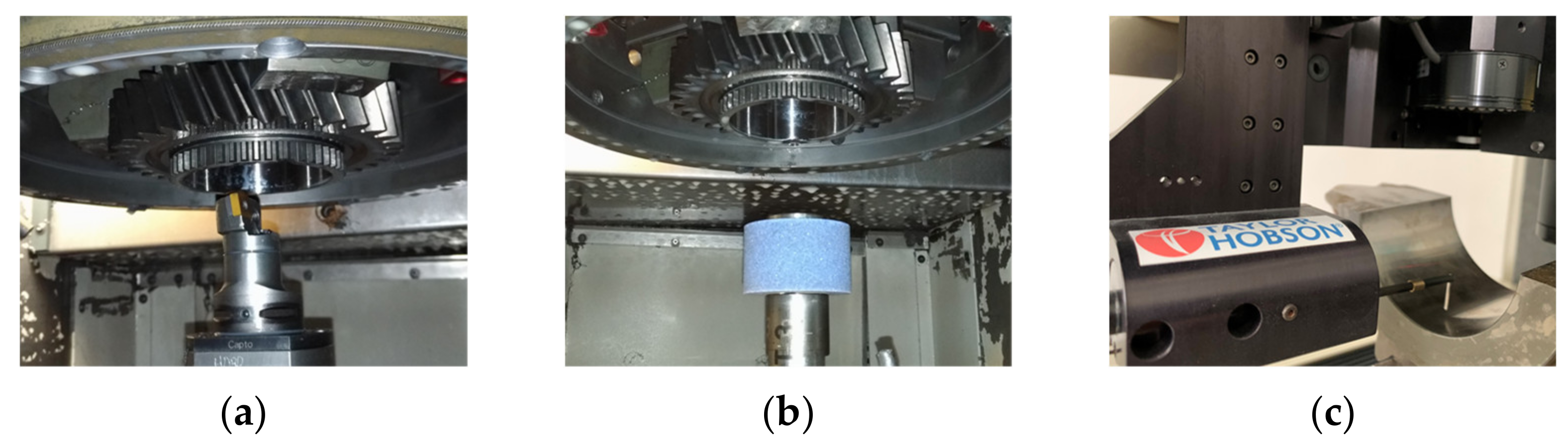
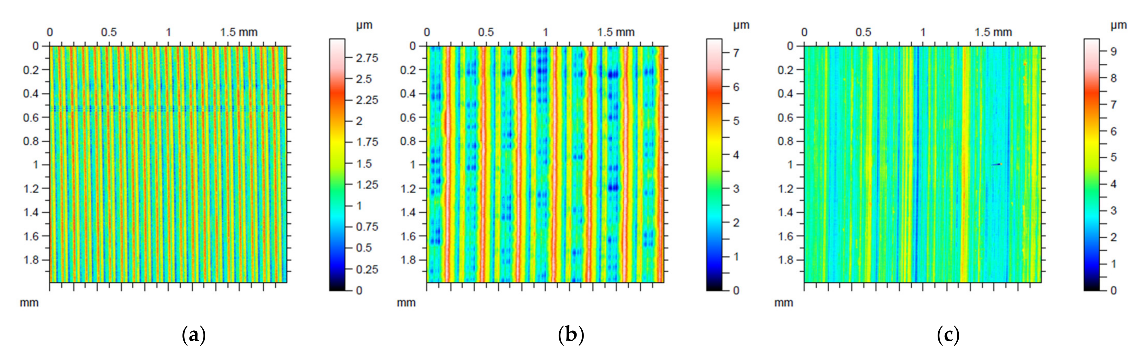
2. Experimental and Measurement Setup
- Turning insert: Sandvik CCGW 09T308 NC2
- Tool holder: E25T-SCLCR 09-R
- Grinding wheel: Norton 3AS80J8VET 01_36X37X13
- Feed: f = 0.1 mm/rev (M1); f = 0.3 mm/rev (M2)
- Depth-of-cut: ap = 0.2 mm
- Workpiece rpm: n = 615 min−1
- Feed: f = 0.01 mm/rev
- Wheel width: L′ = 36 mm
- Infeed depth (radial allowance): Δ = 0.2 mm
- Workpiece rpm: nw = 325 min−1
- Tool rpm: nt = 20,000 min−1
- Arithmetical mean height (Sa, μm): A relatively frequent roughness parameter in part drawings.
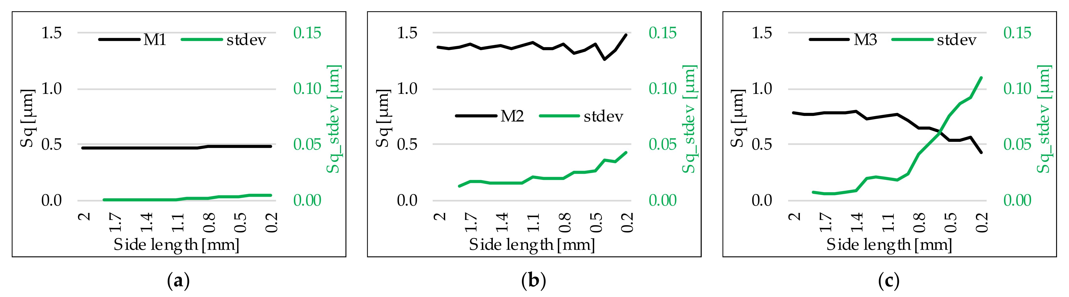
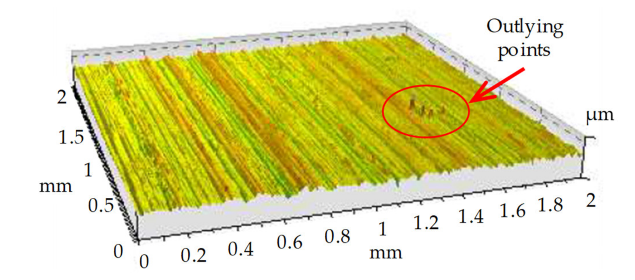
- Root mean square height (Sq, μm): It can be used to qualify the topography of relatively smooth surfaces. It is sensitive to the outlier surface peaks and valleys.
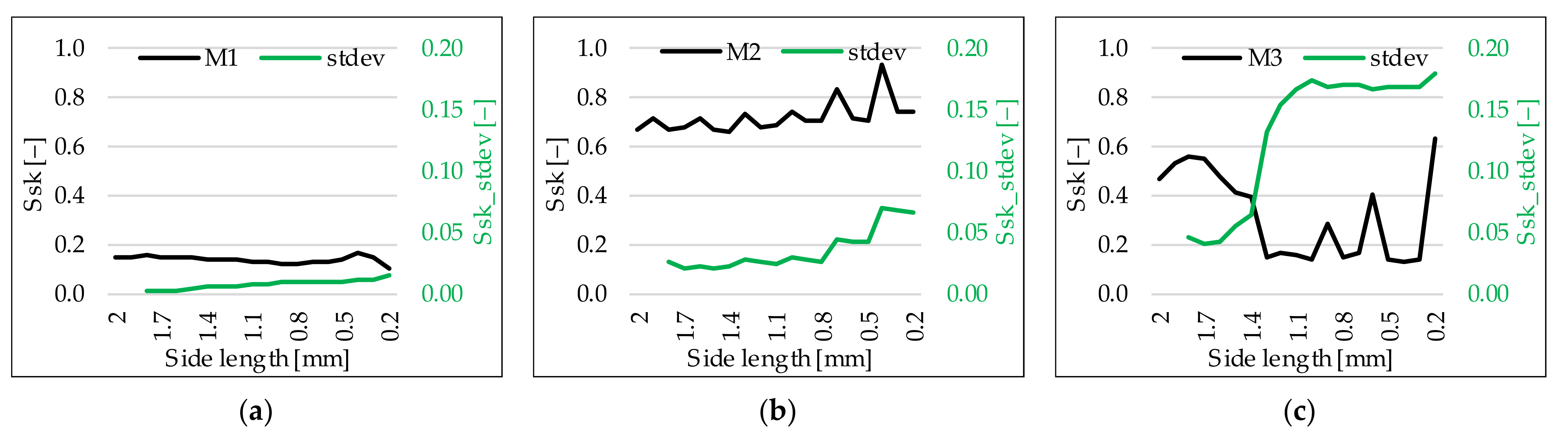
- Skewness (Ssk, –): The working surfaces are characterized by the skewness; it characterizes the tribological properties of the surface. A positive value means the dominance of roughness peaks and a negative value means the dominance of valleys and usually better lubrication.
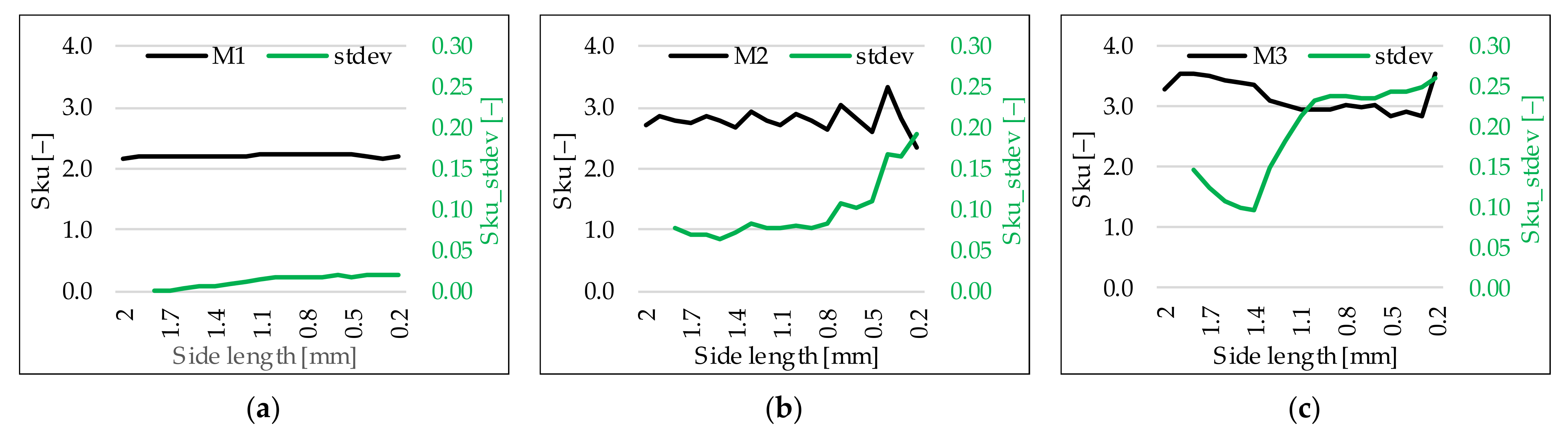
- Kurtosis (Sku, –): It characterizes the tribological properties. It is generally considered together with Ssk. It informs about the lubrication and wear resistance.
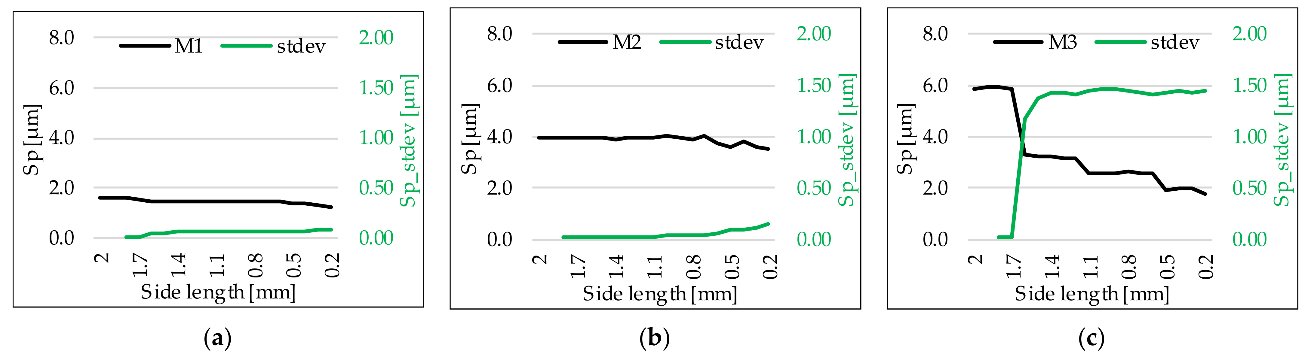
- Maximum peak height (Sp, μm): It is the height of the highest peak within the evaluation area.
- Maximum pit height (Sv, μm): It is the absolute value of the height of the largest pit within the evaluated area.
3. Results and Discussion
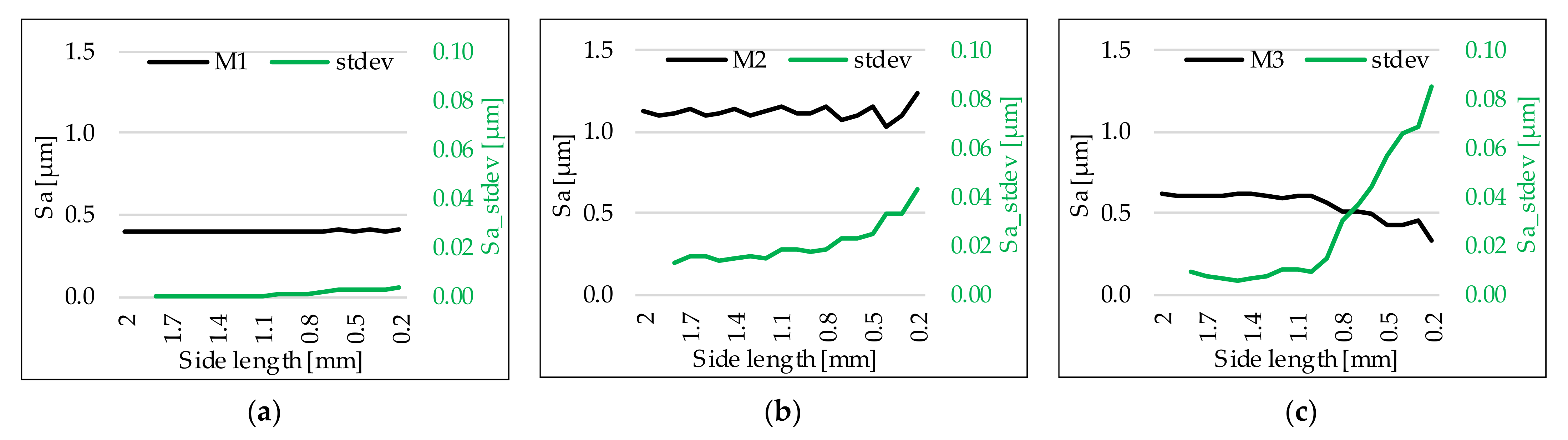
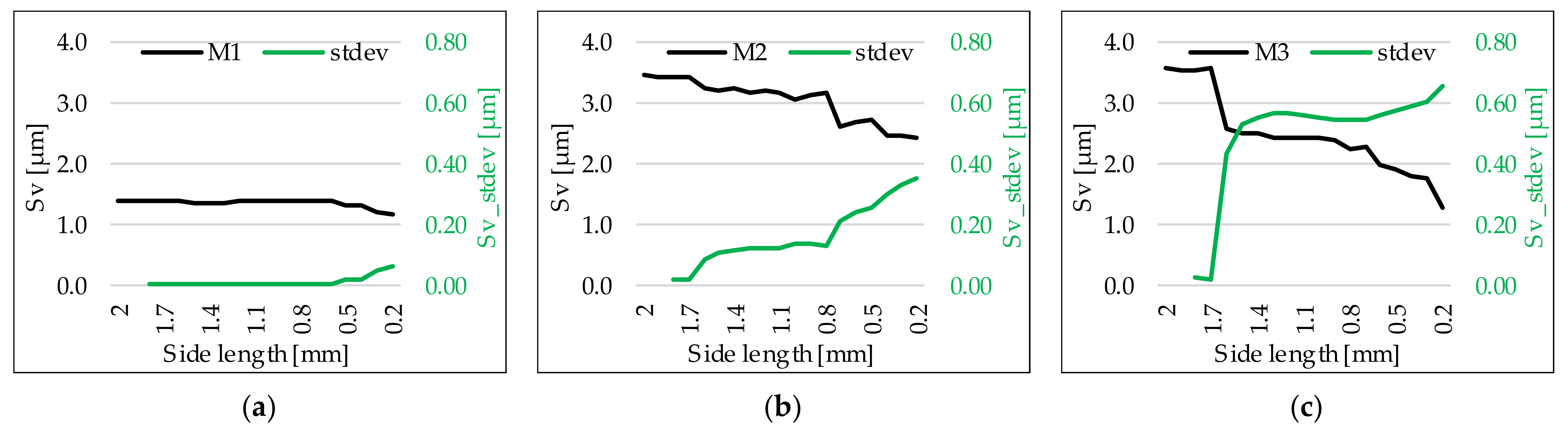
3.1. The Surface Roughness Values and Their Standard Deviations
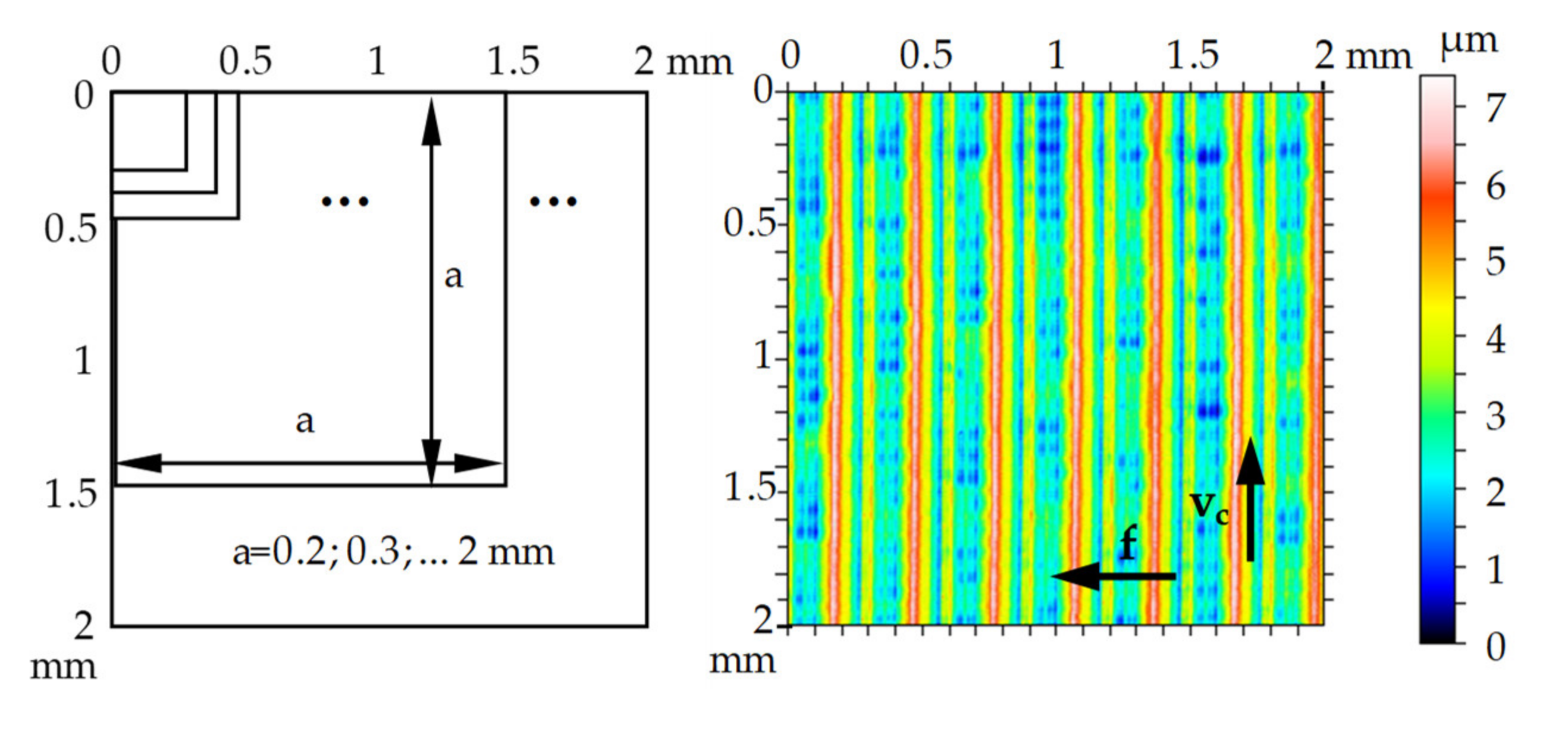
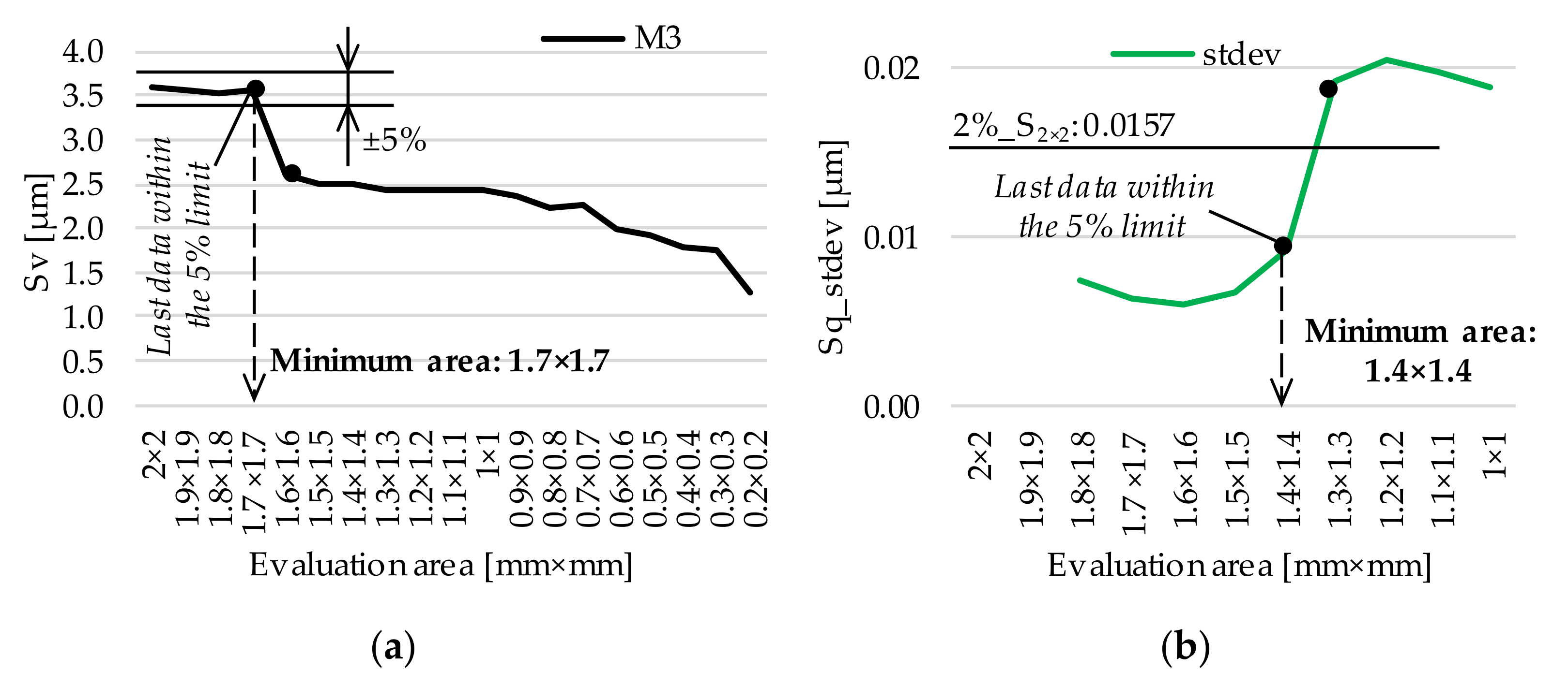
3.2. Designation of Minimum Evaluation Areas
3.3. Validation of the Minimum Evaluation Areas
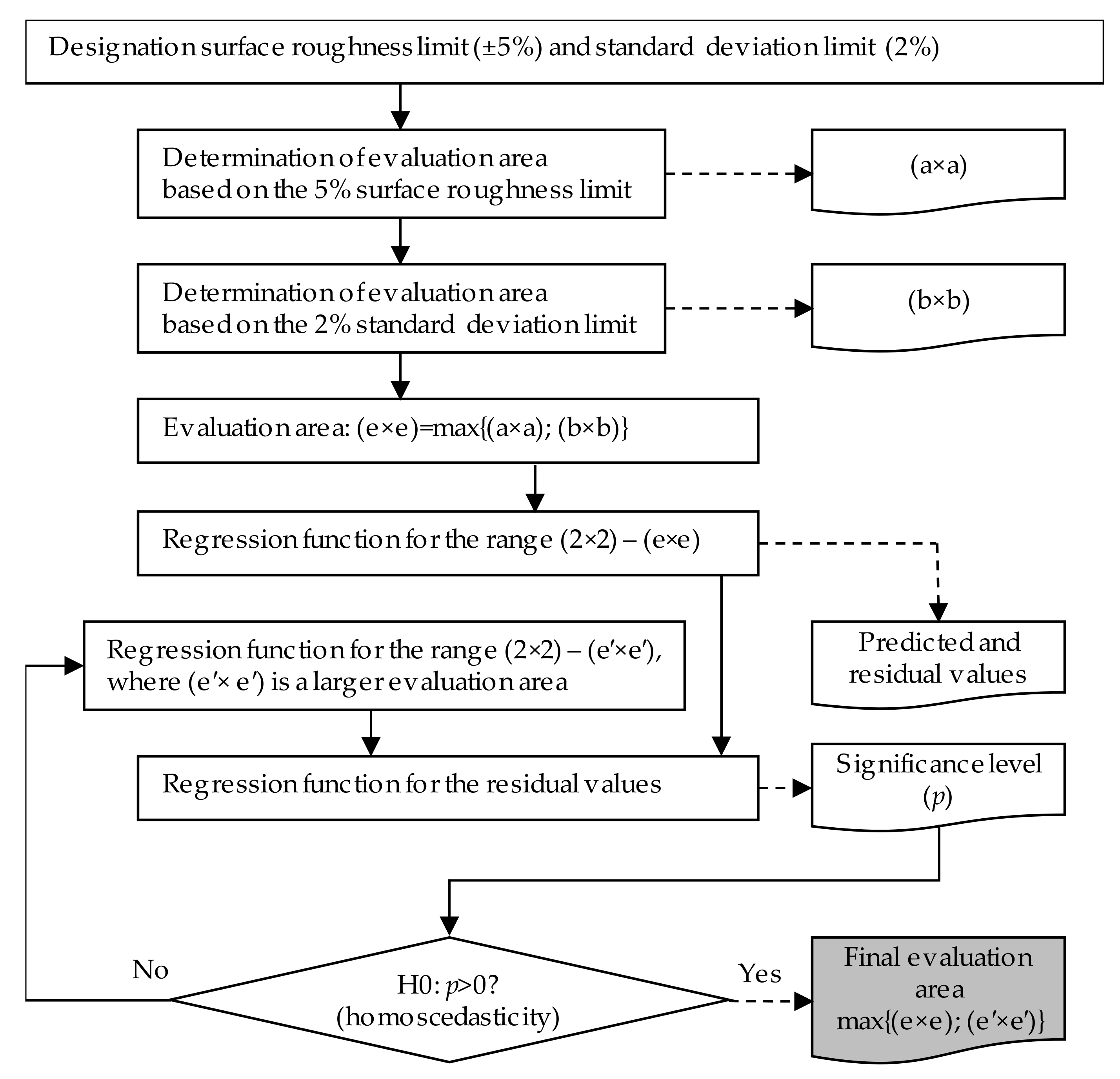
3.3.1. Theoretical Background
3.3.2. Results of the Regression Analysis
4. Conclusions
- There is no clear tendency in the analyzed roughness values when the evaluation area is decreased: the data show oscillation/periodicity (e.g., in the Sa parameter when the surface is hard turned by feed 0.1 mm/rev) in some cases and in others decreasing values (e.g., in the Sq parameter when the surface is machined by infeed grinding) or show irregularities (e.g., in the Sku parameter when the surface is machined by infeed grinding).
- For the Sa, Sq, Sp, and Sv parameters, minimum evaluation areas were determined and validated. Regardless of the machining procedure a 1.3 × 1.3 mm evaluation area can be applied for the Sa parameter, 1.4 × 1.4 mm for Sq, and 1.7 × 1.7 mm for Sp and Sv parameters. These statements are valid only for the analyzed technological data and in the range of surface roughness Sa = 0.4–1.13 μm or Sz = 2.97–9.46 μm.
- Analyzing the Ssk and Sku parameters, valid evaluation areas were determined only in the case of the M1 procedure version (hard turning, f = 0.1 mm/rev). 1.7 × 1.7 mm and 0.4 × 0.4 mm evaluation areas are recommended for the Ssk and the Sku parameters, respectively. In case of the surface hard turned by f = 0.3 mm/rev feed and the ground surface 2 × 2 mm evaluation area is recommended. However, this resulted from the surface roughness and standard deviation limits, and was not validated by the regression analysis.
- Analysis of other machining procedures (e.g., milling, drilling)
- Analysis of the effects of changes in the technological data based on design of experiment.
- Analysis of more or all roughness parameters.
- Calculation of measurement time savings.
Funding
Institutional Review Board Statement
Informed Consent Statement
Data Availability Statement
Conflicts of Interest
Appendix A

| Cutting Technology | Evaluation Area of 3D Roughness Measurement (mm × mm) |
|---|---|
| Burnishing | 2.5 × 2.5 [40], 3.6 × 3.6 [41] |
| Direct Laser Deposition | 1.2 × 0.9 [42] |
| Grinding | 1.2 × 0.9 [42], 1.5 × 1 [43], 2.5 × 2.5 [16], 0.5 × 0.5 [44] |
| Hard turning | 2.5 × 2.5 [40], 0.5 × 0.5 [44], 0.8 × 0.8 [45] |
| Honing | 1.28 × 1.28 [46] |
| Milling | 1.2 × 0.9 [42], 5 × 5 [47], 2.5 × 2.5 [48], 4 × 4 [49] |
| Polishing | 1.9 × 2.5 [50], 1.75 × 1.75 [51] |
| Rolling | 0.7 × 0.525 [52] |
| Turning | 0.705 × 0.528 [53] |
Appendix B
| M1 | Side Length of the Measured Area (Square) (mm) | |||||||||
|---|---|---|---|---|---|---|---|---|---|---|
| 2 | 1.9 | 1.8 | 1.7 | 1.6 | 1.5 | 1.4 | 1.3 | 1.2 | 1.1 | |
| Sa (μm) | 0.398 | 0.398 | 0.398 | 0.397 | 0.397 | 0.397 | 0.398 | 0.398 | 0.398 | 0.398 |
| Sq (μm) | 0.471 | 0.471 | 0.471 | 0.470 | 0.471 | 0.472 | 0.472 | 0.473 | 0.473 | 0.473 |
| Ssk (–) | 0.153 | 0.150 | 0.154 | 0.151 | 0.146 | 0.144 | 0.139 | 0.136 | 0.139 | 0.132 |
| Sku (–) | 2.180 | 2.184 | 2.183 | 2.183 | 2.193 | 2.196 | 2.198 | 2.207 | 2.216 | 2.221 |
| Sp (μm) | 1.582 | 1.575 | 1.573 | 1.568 | 1.491 | 1.457 | 1.454 | 1.452 | 1.451 | 1.445 |
| Sv (μm) | 1.387 | 1.394 | 1.396 | 1.400 | 1.403 | 1.377 | 1.380 | 1.382 | 1.384 | 1.389 |
| M1 | Side Length of the Measured Area (Square) (mm) | |||||||||
| 1 | 0.9 | 0.8 | 0.7 | 0.6 | 0.5 | 0.4 | 0.3 | 0.2 | ||
| Sa (μm) | 0.399 | 0.400 | 0.401 | 0.404 | 0.405 | 0.403 | 0.406 | 0.403 | 0.406 | |
| Sq (μm) | 0.475 | 0.476 | 0.478 | 0.480 | 0.482 | 0.478 | 0.481 | 0.477 | 0.481 | |
| Ssk (–) | 0.132 | 0.125 | 0.123 | 0.128 | 0.128 | 0.138 | 0.168 | 0.146 | 0.104 | |
| Sku (–) | 2.222 | 2.222 | 2.228 | 2.231 | 2.229 | 2.218 | 2.187 | 2.164 | 2.194 | |
| Sp (μm) | 1.438 | 1.432 | 1.426 | 1.425 | 1.428 | 1.411 | 1.411 | 1.281 | 1.247 | |
| Sv (μm) | 1.396 | 1.402 | 1.409 | 1.409 | 1.406 | 1.329 | 1.330 | 1.200 | 1.170 | |
| M2 | Side Length of the Measured Area (Square) (mm) | |||||||||
|---|---|---|---|---|---|---|---|---|---|---|
| 2 | 1.9 | 1.8 | 1.7 | 1.6 | 1.5 | 1.4 | 1.3 | 1.2 | 1.1 | |
| Sa (μm) | 1.127 | 1.102 | 1.119 | 1.140 | 1.105 | 1.114 | 1.139 | 1.102 | 1.127 | 1.158 |
| Sq (μm) | 1.378 | 1.354 | 1.373 | 1.396 | 1.356 | 1.366 | 1.389 | 1.355 | 1.383 | 1.417 |
| Ssk (–) | 0.665 | 0.713 | 0.673 | 0.678 | 0.710 | 0.671 | 0.658 | 0.736 | 0.675 | 0.690 |
| Sku (–) | 2.715 | 2.867 | 2.784 | 2.734 | 2.856 | 2.770 | 2.677 | 2.914 | 2.782 | 2.711 |
| Sp (μm) | 3.936 | 3.985 | 3.957 | 3.951 | 3.977 | 3.925 | 3.899 | 3.979 | 3.935 | 3.942 |
| Sv (μm) | 3.465 | 3.416 | 3.444 | 3.449 | 3.250 | 3.211 | 3.237 | 3.158 | 3.201 | 3.157 |
| M2 | Side Length of the Measured Area (Square) (mm) | |||||||||
| 1 | 0.9 | 0.8 | 0.7 | 0.6 | 0.5 | 0.4 | 0.3 | 0.2 | ||
| Sa (μm) | 1.106 | 1.109 | 1.150 | 1.069 | 1.095 | 1.159 | 1.024 | 1.093 | 1.240 | |
| Sq (μm) | 1.358 | 1.363 | 1.402 | 1.316 | 1.346 | 1.406 | 1.269 | 1.344 | 1.475 | |
| Ssk (–) | 0.742 | 0.701 | 0.701 | 0.831 | 0.718 | 0.708 | 0.935 | 0.746 | 0.741 | |
| Sku (–) | 2.902 | 2.794 | 2.652 | 3.042 | 2.807 | 2.597 | 3.324 | 2.810 | 2.355 | |
| Sp (μm) | 4.030 | 3.950 | 3.924 | 4.012 | 3.775 | 3.628 | 3.792 | 3.613 | 3.491 | |
| Sv (μm) | 3.070 | 3.145 | 3.171 | 2.639 | 2.711 | 2.721 | 2.480 | 2.459 | 2.447 | |
| M3 | Side Length of the Measured Area (Square) (mm) | |||||||||
|---|---|---|---|---|---|---|---|---|---|---|
| 2 | 1.9 | 1.8 | 1.7 | 1.6 | 1.5 | 1.4 | 1.3 | 1.2 | 1.1 | |
| Sa (μm) | 0.621 | 0.603 | 0.608 | 0.611 | 0.611 | 0.615 | 0.622 | 0.600 | 0.589 | 0.602 |
| Sq (μm) | 0.784 | 0.769 | 0.776 | 0.780 | 0.782 | 0.788 | 0.798 | 0.734 | 0.747 | 0.760 |
| Ssk (–) | 0.468 | 0.528 | 0.557 | 0.550 | 0.474 | 0.415 | 0.394 | 0.150 | 0.164 | 0.155 |
| Sku (–) | 3.279 | 3.526 | 3.537 | 3.513 | 3.436 | 3.394 | 3.363 | 3.097 | 3.045 | 2.949 |
| Sp (μm) | 5.862 | 5.901 | 5.918 | 5.896 | 3.269 | 3.229 | 3.221 | 3.173 | 3.171 | 2.598 |
| Sv (μm) | 3.598 | 3.559 | 3.542 | 3.565 | 2.591 | 2.499 | 2.507 | 2.435 | 2.438 | 2.431 |
| M3 | Side Length of the Measured Area (Square) (mm) | |||||||||
| 1 | 0.9 | 0.8 | 0.7 | 0.6 | 0.5 | 0.4 | 0.3 | 0.2 | ||
| Sa (μm) | 0.605 | 0.566 | 0.510 | 0.510 | 0.493 | 0.430 | 0.428 | 0.454 | 0.335 | |
| Sq (μm) | 0.766 | 0.715 | 0.643 | 0.641 | 0.621 | 0.538 | 0.534 | 0.561 | 0.433 | |
| Ssk (–) | 0.139 | 0.288 | 0.150 | 0.163 | 0.402 | 0.135 | 0.135 | 0.144 | 0.632 | |
| Sku (–) | 2.943 | 2.966 | 3.031 | 2.994 | 3.010 | 2.853 | 2.906 | 2.848 | 3.554 | |
| Sp (μm) | 2.597 | 2.542 | 2.621 | 2.588 | 2.580 | 1.936 | 1.982 | 2.010 | 1.742 | |
| Sv (μm) | 2.432 | 2.382 | 2.241 | 2.274 | 1.993 | 1.912 | 1.792 | 1.764 | 1.282 | |
Appendix C

References
- Bławucki, S.; Zaleski, K. The effect of the aluminium alloy surface roughness on the restitution coefficient. Adv. Sci. Technol. Res. J. 2015, 9, 66–71. [Google Scholar] [CrossRef][Green Version]
- Gogolin, A.; Wasilewski, M.; Ligus, G.; Wojciechowski, S.; Gapinski, B.; Krolczyk, J.; Zajac, D.; Krolczyk, G. Influence of geometry and surface morphology of the U-tube on the fluid flow in the range of various velocities. Measurement 2020, 164, 108094. [Google Scholar] [CrossRef]
- Felho, C.; Kundrák, J. Characterization of Topography of Cut Surface Based on Theoretical Roughness Indexes. Key Eng. Mater. 2012, 496, 194–199. [Google Scholar] [CrossRef]
- Sztankovics, I.; Kundrák, J. Theoretical Value of Total Height of Profile in Rotational Turning. Appl. Mech. Mater. 2013, 309, 154–161. [Google Scholar] [CrossRef]
- Kundrak, J.; Felho, C. 3D Roughness Parameters of Surfaces Face Milled by Special Tools. Manuf. Technol. 2016, 16, 532–538. [Google Scholar] [CrossRef]
- Mamalis, A.G.; Kundrak, J. Horvath M: On a novel tool life relation for precision cutting tools. J. Manuf. Sci. Eng. 2005, 127, 328–332. [Google Scholar] [CrossRef]
- Karkalos, N.E.; Karmiris-Obratanski, P.; Kurpiel, S.; Zagorski, K.; Markopoulos, A.P. Investigation on the surface quality obtained during trochoidal milling of 6082 aluminum alloy. Machines 2021, 9, 75. [Google Scholar] [CrossRef]
- Sagbas, A. Analysis and optimization of surface roughness in the ball burnishing process using response surface methodology and desirabilty function. Adv. Eng. Softw. 2011, 42, 992–998. [Google Scholar] [CrossRef]
- Przestacki, D.; Majchrowski, R.; Marciniak-Podsadna, L. Experimental research of surface roughness and surface texture after laser cladding. Appl. Surf. Sci. 2016, 388, 420–423. [Google Scholar] [CrossRef]
- Kumar, R.; Seetharamu, S.; Kamaraj, M. Quantitative evaluation of 3D surface roughness parameters during cavitation exposure of 16Cr–5Ni hydro turbine steel. Wear 2014, 320, 16–24. [Google Scholar] [CrossRef]
- Aidibe, A.; Nejad, M.K.; Tahan, A.; Jahazi, M.; Cloutier, S.G. A Proposition for New Quality 3D Indexes to Measure Surface Roughness. Procedia CIRP 2016, 46, 327–330. [Google Scholar] [CrossRef][Green Version]
- Linins, O.; Krizbergs, J.; Boiko, I. Surface texture metrology gives a better understanding of the surface in its functional state. Key Eng. Mater 2013, 527, 167–172. [Google Scholar] [CrossRef]
- Khellaf, A.; Aouici, H.; Smaiah, S.; Boutabba, S.; Yallese, M.A.; Elbah, M. Comparative assessment of two ceramic cutting tools on surface roughness in hard turning of AISI H11 steel: Including 2D and 3D surface topography. Int. J. Adv. Manuf. Technol. 2016, 89, 333–354. [Google Scholar] [CrossRef]
- Elbah, M.; Laouici, H.; Benlahmidi, S.; Nouioua, M.; Yallese, M. Comparative assessment of machining environments (dry, wet and MQL) in hard turning of AISI 4140 steel with CC6050 tools. Int. J. Adv. Manuf. Technol. 2019, 105, 2581–2597. [Google Scholar] [CrossRef]
- Li, S.; Chen, T.; Qiu, C.; Wang, D.; Liu, X. Experimental investigation of high-speed hard turning by PCBN tooling with strengthened edge. Int. J. Adv. Manuf. Technol. 2017, 92, 3785–3793. [Google Scholar] [CrossRef]
- Legutko, S.; Zak, K.; Kudlaček, J. Characteristics of geometric structure of the surface after grinding. MATEC Web Conf. 2017, 94, 2007. [Google Scholar] [CrossRef][Green Version]
- John, J.G.; Arunachalam, N. Illumination Compensated images for surface roughness evaluation using machine vision in grinding process. Procedia Manuf. 2019, 34, 969–977. [Google Scholar] [CrossRef]
- Zhu, L.; Guan, Y.; Wang, Y.; Xie, Z.; Lin, J.; Zhai, J. Influence of process parameters of ultrasonic shot peening on surface roughness and hydrophilicity of pure titanium. Surf. Coat. Technol. 2017, 317, 38–53. [Google Scholar] [CrossRef]
- Mesicek, J.; Ma, Q.-P.; Hajnys, J.; Zelinka, J.; Pagac, M.; Petru, J.; Mizera, O. Abrasive Surface Finishing on SLM 316L Parts Fabricated with Recycled Powder. Appl. Sci. 2021, 11, 2869. [Google Scholar] [CrossRef]
- Zhao, T.; Zhou, J.M.; Bushlya, V.; Ståhl, J.E. Effect of cutting edge radius on surface roughness and tool wear in hard turning of AISI 52100 steel. Int. J. Adv. Manuf. Technol. 2017, 91, 3611–3618. [Google Scholar] [CrossRef]
- Gao, H.; Ma, B.; Singh, R.P.; Yang, H. Areal Surface Roughness of AZ31B Magnesium Alloy Processed by Dry Face Turning: An Experimental Framework Combined with Regression Analysis. Materials 2020, 13, 2303. [Google Scholar] [CrossRef] [PubMed]
- Schwartzentruber, J.; Spelt, J.; Papini, M. Prediction of surface roughness in abrasive waterjet trimming of fiber reinforced polymer composites. Int. J. Mach. Tools Manuf. 2017, 122, 1–17. [Google Scholar] [CrossRef]
- Kumaran, S.T.; Ko, T.J.; Uthayakumar, M.; Islam, M. Prediction of surface roughness in abrasive water jet machining of CFRP composites using regression analysis. J. Alloys Compd. 2017, 724, 1037–1045. [Google Scholar] [CrossRef]
- He, C.; Zong, W.; Sun, T. Origins for the size effect of surface roughness in diamond turning. Int. J. Mach. Tools Manuf. 2016, 106, 22–42. [Google Scholar] [CrossRef]
- Lu, X.; Hu, X.; Jia, Z.; Liu, M.; Gao, S.; Qu, C.; Liang, S.Y. Model for the prediction of 3D surface topography and surface roughness in micro-milling Inconel 718. Int. J. Adv. Manuf. Technol. 2017, 94, 2043–2056. [Google Scholar] [CrossRef]
- Charles, A.; Elkaseer, A.; Thijs, L.; Hagenmeyer, V.; Scholz, S. Effect of process parameters on the generated surface rough-ness of down-facing surfaces in selective laser melting. Appl. Sci. 2019, 9, 1256. [Google Scholar] [CrossRef]
- Kuo, C.; Nien, Y.; Chiang, A.; Hirata, A. Surface modification using assisting electrodes in wire electrical discharge machining for silicon wafer preparation. Materials 2021, 14, 1355. [Google Scholar] [CrossRef]
- Pan, C.; Li, Q.; Hu, K.; Jiao, Y.; Song, Y. Study on Surface Roughness of Gcr15 Machined by Micro-Texture PCBN Tools. Machines 2018, 6, 42. [Google Scholar] [CrossRef]
- Deja, M.; Markopoulos, A. Advances and Trends in Non-Conventional, Abrasive and Precision Machining. Machines 2021, 9, 37. [Google Scholar] [CrossRef]
- Tapoglou, N. Development of Cutting Force Model and Process Maps for Power Skiving Using CAD-Based Modelling. Machines 2021, 9, 95. [Google Scholar] [CrossRef]
- Yong, Q.; Chang, J.; Liu, Q.; Jiang, F.; Wei, D.; Li, H. Matt polyurethane coating: Correlation of surface roughness on measurement length and gloss. Polymers 2020, 12, 326. [Google Scholar] [CrossRef] [PubMed]
- Zawada-Tomkiewicz, A. Analysis of surface roughness parameters achieved by hard turning with the use of PCBN tools. Estonian J. Eng. 2011, 17, 88. [Google Scholar] [CrossRef]
- Pyka, G.; Kerckhofs, G.; Papantoniou, I.; Speirs, M.; Schrooten, J.; Wevers, M. Surface roughness and morphology customization of additive manufactured open porous Ti6Al4V structures. Materials 2013, 6, 4737–4757. [Google Scholar] [CrossRef]
- Pytlak, B. The roughness parameters 2D and 3D and some characteristics of the machined surface topography after hard turning and grinding of hardened 18CrMo4 steel. Kom. Budowy Masz. Pan–Oddz. W Pozn. 2011, 31, 53–62. [Google Scholar]
- Sun, Y.; Jin, L.; Gong, Y.; Qi, Y.; Zhang, H.; Su, Z.; Sun, K. Experimental Investigation on Machinability of Aluminum Alloy during Dry Micro Cutting Process Using Helical Micro End Mills with Micro Textures. Materials 2020, 13, 4664. [Google Scholar] [CrossRef] [PubMed]
- Abouelatta, O.B. 3D Surface roughness measurement using a light sectioning vision system. In Proceedings of the World Con-gress on Engineering, London, UK, 30 June–2 July 2010; Volume 1. [Google Scholar]
- Shivanna, D.; Kiran, M.; Kavitha, S. Evaluation of 3D Surface Roughness Parameters of EDM Components Using Vision System. Procedia Mater. Sci. 2014, 5, 2132–2141. [Google Scholar] [CrossRef]
- Kluz, R.; Antosz, K.; Trzepieciński, T.; Bucior, M. Modelling the Influence of Slide Burnishing Parameters on the Surface Roughness of Shafts Made of 42CrMo4 Heat-Treatable Steel. Materials 2021, 14, 1175. [Google Scholar] [CrossRef] [PubMed]
- Zaman, A. Statistical Foundations for Econometric Techniques; Academic Press: New York, NY, USA, 1996. [Google Scholar]
- Grzesik, W.; Rech, J.; Żak, K. High-precision Finishing Hard Steel Surfaces Using Cutting, Abrasive and Burnishing Operations. Procedia Manuf. 2015, 1, 619–627. [Google Scholar] [CrossRef]
- Dzierwa, A.; Markopoulos, A.P. Influence of Ball-Burnishing Process on Surface Topography Parameters and Tribological Properties of Hardened Steel. Machines 2019, 7, 11. [Google Scholar] [CrossRef]
- Wojciechowski, S.; Twardowski, P.; Chwalczuk, T. Surface roughness analysis after machining of direct laser deposited tungsten carbide. J. Phys. Conf. Ser. 2014, 483, 012018. [Google Scholar] [CrossRef]
- Schmahling, J.; Hamprecht, F.A.; Hoffmann, D.M.P. A three-dimensional measure of surface roughness based on mathematical morphology. In Technical Report from Multidimensional Image Processing, IWR; University of Heidelberg: Heidelberg, Germany, 2006. [Google Scholar]
- Grzesik, W.; Żak, K.; Kiszka, P. Comparison of Surface Textures Generated in Hard Turning and Grinding Operations. Procedia CIRP 2014, 13, 84–89. [Google Scholar] [CrossRef]
- Matras, A.; Zębala, W.; Machno, M. Research and Method of Roughness Prediction of a Curvilinear Surface after Titanium Alloy Turning. Materials 2019, 12, 502. [Google Scholar] [CrossRef] [PubMed]
- Karolczak, P.; Kowalski, M.; Wiśniewska, M. Analysis of the Possibility of Using Wavelet Transform to Assess the Condition of the Surface Layer of Elements with Flat-Top Structures. Machines 2020, 8, 65. [Google Scholar] [CrossRef]
- Nadolny, K.; Kaplonek, W. Analysis of flatness deviations for austenitic stainless-steel workpieces after efficient surface machining. Meas. Sci. Rev. 2014, 14, 204. [Google Scholar] [CrossRef]
- Kundrak, J.; Nagy, A.; Markopoulos, A.P.; Karkalos, N.E. Investigation of surface roughness on face milled parts with round insert in planes parallel to the feed at various cutting speeds. Cut. Tools Technol. Syst. 2019, 87–96. [Google Scholar] [CrossRef]
- Chuchala, D.; Dobrzynski, M.; Pimenov, D.; Orlowski, K.; Krolczyk, G.; Giasin, K. Surface Roughness Evaluation in Thin EN AW-6086-T6 Alloy Plates after Face Milling Process with Different Strategies. Materials 2021, 14, 3036. [Google Scholar] [CrossRef] [PubMed]
- Zhou, H.; Zhou, H.; Zhao, Z.; Li, K.; Yin, J. Numerical Simulation and Verification of Laser-Polishing Free Surface of S136D Die Steel. Metals 2021, 11, 400. [Google Scholar] [CrossRef]
- Zhou, J.; Han, X.; Li, H.; Liu, S.; Shen, S.; Zhou, X.; Zhang, D. In-Situ Laser Polishing Additive Manufactured AlSi10Mg: Effect of Laser Polishing Strategy on Surface Morphology, Roughness and Microhardness. Materials 2021, 14, 393. [Google Scholar] [CrossRef]
- Deltombe, R.; Kubiak, K.J.; Bigerelle, M. How to select the most relevant 3D roughness parameters of a surface? Scanning 2014, 36, 150–160. [Google Scholar] [CrossRef]
- Struzikiewicz, G.; Sioma, A. Evaluation of Surface Roughness and Defect Formation after The Machining of Sintered Aluminum Alloy AlSi10Mg. Materials 2020, 13, 1662. [Google Scholar] [CrossRef]


| Yield Strength σs (MPa) | Tensile Strength σb (MPa) | Hardness HRC | Thermal Conductivity k (W/mK) | Density ρ (g/cm3) | Elastic Modulus E (GPa) |
|---|---|---|---|---|---|
| 1034 | 1158 | 62–64 | 11.7 | 7.7–8.03 | 190–210 |
| C | Si | Mp | S | P | Cr | Cu | Al |
|---|---|---|---|---|---|---|---|
| 0.17–0.22 | ≤0.4 | 1.1–1.4 | ≤0.035 | ≤0.025 | 1.0–1.3 | ≤0.4 | 0.02–0.04 |
| Side Length of the Measured Area (Square) (mm) | ||||||||||||||||||||
|---|---|---|---|---|---|---|---|---|---|---|---|---|---|---|---|---|---|---|---|---|
| 2.0 | 1.9 | 1.8 | 1.7 | 1.6 | 1.5 | 1.4 | 1.3 | 1.2 | 1.1 | 1.0 | 0.9 | 0.8 | 0.7 | 0.6 | 0.5 | 0.4 | 0.3 | 0.2 | ||
| Sa (μm) | M1 | 0.0 | 0.1 | 0.1 | 0.2 | 0.2 | 0.1 | 0.0 | 0.1 | 0.1 | 0.0 | 0.3 | 0.5 | 0.9 | 1.5 | 1.9 | 1.3 | 2.0 | 1.4 | 2.0 |
| M2 | 0.0 | 2.2 | 0.8 | 1.1 | 2.0 | 1.2 | 1.0 | 2.2 | 0.0 | 2.8 | 1.9 | 1.6 | 2.0 | 5.1 | 2.9 | 2.8 | 9.2 | 3.0 | 10 | |
| M3 | 0.0 | 2.9 | 2.2 | 1.6 | 1.6 | 1.0 | 0.1 | 3.4 | 5.2 | 3.0 | 2.6 | 8.9 | 18 | 18 | 21 | 31 | 31 | 27 | 46 | |
| Sq (μm) | M1 | 0.0 | 0.0 | 0.1 | 0.2 | 0.1 | 0.0 | 0.1 | 0.3 | 0.4 | 0.4 | 0.7 | 0.9 | 1.4 | 1.9 | 2.2 | 1.4 | 2.1 | 1.1 | 2.1 |
| M2 | 0.0 | 1.8 | 0.4 | 1.3 | 1.6 | 0.9 | 0.8 | 1.7 | 0.3 | 2.8 | 1.5 | 1.1 | 1.7 | 4.5 | 2.3 | 2.0 | 7.9 | 2.5 | 7.0 | |
| M3 | 0.0 | 1.9 | 1.0 | 0.6 | 0.2 | 0.5 | 1.8 | 6.4 | 4.7 | 3.0 | 2.3 | 8.8 | 18 | 18 | 21 | 31 | 32 | 28 | 45 | |
| Ssk (–) | M1 | 0.0 | 2.0 | 0.7 | 1.5 | 4.6 | 5.6 | 9.0 | 11 | 9.3 | 14 | 13 | 18 | 20 | 16 | 16 | 10 | 10 | 4.8 | 32 |
| M2 | 0.0 | 7.1 | 1.2 | 1.9 | 6.8 | 0.8 | 1.1 | 11 | 1.5 | 3.7 | 12 | 5.3 | 5.4 | 25 | 7.9 | 6.4 | 41 | 12 | 11 | |
| M3 | 0.0 | 13 | 19 | 17 | 1.2 | 11 | 16 | 68 | 65 | 67 | 70 | 38 | 68 | 65 | 14 | 71 | 71 | 69 | 35 | |
| Sku (–) | M1 | 0.0 | 0.2 | 0.1 | 0.1 | 0.6 | 0.7 | 0.8 | 1.2 | 1.6 | 1.9 | 1.9 | 1.9 | 2.2 | 2.3 | 2.2 | 1.7 | 0.3 | 0.7 | 0.6 |
| M2 | 0.0 | 5.6 | 2.5 | 0.7 | 5.2 | 2.0 | 1.4 | 7.3 | 2.5 | 0.1 | 6.9 | 2.9 | 2.3 | 12 | 3.4 | 4.4 | 22 | 3.5 | 13 | |
| M3 | 0.0 | 7.5 | 7.9 | 7.1 | 4.8 | 3.5 | 2.6 | 5.5 | 7.1 | 10 | 10 | 10 | 7.6 | 8.7 | 8.2 | 13 | 11 | 13 | 8.4 | |
| Sp (μm) | M1 | 0.0 | 0.4 | 0.6 | 0.9 | 5.8 | 7.9 | 8.1 | 8.2 | 8.3 | 8.6 | 9.1 | 9.5 | 10 | 10 | 10 | 11 | 11 | 19 | 21 |
| M2 | 0.0 | 1.2 | 0.5 | 0.4 | 1.1 | 0.3 | 0.9 | 1.1 | 0.0 | 0.2 | 2.4 | 0.4 | 0.3 | 1.9 | 4.1 | 7.8 | 3.6 | 8.2 | 11 | |
| M3 | 0.0 | 0.7 | 1.0 | 0.6 | 44 | 45 | 45 | 46 | 46 | 56 | 56 | 57 | 55 | 56 | 56 | 67 | 66 | 66 | 70 | |
| Sv (μm) | M1 | 0.0 | 0.5 | 0.6 | 1.0 | 1.1 | 0.7 | 0.5 | 0.4 | 0.2 | 0.1 | 0.6 | 1.1 | 1.6 | 1.6 | 1.4 | 4.2 | 4.1 | 13 | 16 |
| M2 | 0.0 | 1.4 | 0.6 | 0.5 | 6.2 | 7.3 | 6.6 | 8.9 | 7.6 | 8.9 | 11 | 9.3 | 8.5 | 24 | 22 | 21 | 28 | 29 | 29 | |
| M3 | 0.0 | 1.1 | 1.6 | 0.9 | 28 | 31 | 30 | 32 | 32 | 32 | 32 | 34 | 38 | 37 | 45 | 47 | 50 | 51 | 64 | |
| Roughness parameters and machining procedures | Sa (μm) | Sa (μm) | Sa (μm) | Sq (μm) | Sq (μm) | Sq (μm) | Ssk (–) | Ssk (–) | Ssk (–) |
|---|---|---|---|---|---|---|---|---|---|
| M1 | M2 | M3 | M1 | M2 | M3 | M1 | M2 | M3 | |
| Roughness of the 2 × 2 mm area | 0.398 | 1.127 | 0.621 | 0.471 | 1.378 | 0.784 | 0.153 | 0.666 | 0.468 |
| 2% of the roughness value | 0.008 | 0.023 | 0.012 | 0.009 | 0.028 | 0.016 | 0.003 | 0.013 | 0.009 |
| Last stdev below the 2% limit | 0.003 | 0.019 | 0.010 | 0.000 | 0.000 | 0.009 | 0.002 | – | – |
| Minimum evaluation area (mm × mm) | 0.2 × 0.2 | 0.8 × 0.8 | 1 × 1 | 0.2 × 0.2 | 0.5 × 0.5 | 1.4 × 1.4 | 1.7 × 1.7 | – | – |
| Roughness parameters and machining procedures | Sku (–) | Sku (–) | Sku (–) | Sp (μm) | Sp (μm) | Sp (μm) | Sv (μm) | Sv (μm) | Sv (μm) |
| M1 | M2 | M3 | M1 | M2 | M3 | M1 | M2 | M3 | |
| Roughness of the 2 × 2 mm area | 2.180 | 2.713 | 3.279 | 1.582 | 3.936 | 5.862 | 1.387 | 3.465 | 3.598 |
| 2% of the roughness value | 0.044 | 0.054 | 0.066 | 0.032 | 0.079 | 0.117 | 0.028 | 0.069 | 0.072 |
| Last stdev below the 2% limit | 0.020 | – | – | 0.006 | 0.058 | 0.024 | 0.023 | 0.021 | 0.027 |
| Minimum evaluation area (mm × mm) | 0.2 × 0.2 | – | – | 1.7 × 1.7 | 0.6 × 0.6 | 1.7 × 1.7 | 0.4 × 0.4 | 1.7 × 1.7 | 1.7 × 1.7 |
| Surface Roughness Parameter | Machining Procedure | Minimum Evaluation Area (mm × mm) | Significance Level (p) | ||
|---|---|---|---|---|---|
| 5% Limit (Surface Roughness) | 2% Limit (Standard Deviation) | Regression Analyses | |||
| Sa (μm) | M1 | 0.2 × 0.2 | 0.2 × 0.2 | 0.2 × 0.2 | 0.823 |
| M2 | 0.8 × 0.8 | 0.8 × 0.8 | 0.8 × 0.8 | 0.099 | |
| M3 | 1.3 × 1.3 | 1 × 1 | 1.3 × 1.3 | 0.512 | |
| Sq (μm) | M1 | 0.2 × 0.2 | 0.2 × 0.2 | 0.2 × 0.2 | 0.089 |
| M2 | 0.5 × 0.5 | 0.5 × 0.5 | 0.6 × 0.6 | 0.122 | |
| M3 | 1.4 × 1.4 | 1.4 × 1.4 | 1.4 × 1.4 | 0.122 | |
| Ssk (–) | M1 | 1.6 × 1.6 | 1.7 × 1.7 | 1.7 × 1.7 | 0.909 |
| M2 | 2 × 2 | – | 2 × 2 | – | |
| M3 | 2 × 2 | – | 2 × 2 | – | |
| Sku (–) | M1 | 0.2 × 0.2 | 0.2 × 0.2 | 0.4 × 0.4 | 0.059 |
| M2 | 2 × 2 | – | 2 × 2 | – | |
| M3 | 2 × 2 | – | 2 × 2 | – | |
| Sp (μm) | M1 | 1.7 × 1.7 | 1.7 × 1.7 | 1.7 × 1.7 | 0.068 |
| M2 | 0.6 × 0.6 | 0.6 × 0.6 | 0.7 × 0.7 | 0.167 | |
| M3 | 1.7 × 1.7 | 1.7 × 1.7 | 1.7 × 1.7 | 0.401 | |
| Sv (μm) | M1 | 0.4 × 0.4 | 0.4 × 0.4 | 0.6 × 0.6 | 0.576 |
| M2 | 1.7 × 1.7 | 1.7 × 1.7 | 1.7 × 1.7 | 0.430 | |
| M3 | 1.7 × 1.7 | 1.7 × 1.7 | 1.7 × 1.7 | 0.401 | |
Publisher’s Note: MDPI stays neutral with regard to jurisdictional claims in published maps and institutional affiliations. |
© 2021 by the author. Licensee MDPI, Basel, Switzerland. This article is an open access article distributed under the terms and conditions of the Creative Commons Attribution (CC BY) license (https://creativecommons.org/licenses/by/4.0/).
Share and Cite
Molnár, V. Minimization Method for 3D Surface Roughness Evaluation Area. Machines 2021, 9, 192. https://doi.org/10.3390/machines9090192
Molnár V. Minimization Method for 3D Surface Roughness Evaluation Area. Machines. 2021; 9(9):192. https://doi.org/10.3390/machines9090192
Chicago/Turabian StyleMolnár, Viktor. 2021. "Minimization Method for 3D Surface Roughness Evaluation Area" Machines 9, no. 9: 192. https://doi.org/10.3390/machines9090192
APA StyleMolnár, V. (2021). Minimization Method for 3D Surface Roughness Evaluation Area. Machines, 9(9), 192. https://doi.org/10.3390/machines9090192