Combined Optimization Prediction Model of Regional Wind Power Based on Convolution Neural Network and Similar Days

Abstract

With the continuous optimization of energy structures, wind power generation has become the dominant new energy source. The strong random fluctuation of natural wind will bring challenges to power system dispatching, so it is necessary to predict wind power. In order to improve the short-term prediction accuracy of regional wind power, this paper proposes a new combination prediction model based on convolutional neural network (CNN) and similar days analysis. Firstly, the least square fitting and batch normalization (BN) are used to preprocess the data, and then the recent historical wind power data set for CNN is established. Secondly, the Pearson correlation coefficient and cosine similarity combination method are utilized to find similar days in the long-term data set, and the prediction model based on similar days is constructed by the weighting method. Finally, based on the particle swarm optimization (PSO) method, a combined forecasting model is established. The results show that the combined model can accurately predict the future short-term wind power curve, and the prediction accuracy is improved to different extents compared to a single method.

1. Introduction

In recent years, the new energy input, dominated by wind power generation, is increasing rapidly. The strong volatility and randomness of natural wind make it difficult to accurately predict wind power, which brings new problems for the safe and stable operation of power grids [1,2]. More and more researchers have been committed to investigating the best model to predict the wind power. Generally speaking, model complexity is an index to measure the quality of the model and the simple one is preferred. Traditional methods [3,4], such as the autoregressive moving average model (ARMA) and grey model, cannot dig deeper into the law, which leads to low prediction accuracy. Thus, the common way for high accuracy is to increase the complexity of the model. With the continuous development of artificial intelligence technology, wind power prediction based on machine learning [5,6,7,8] and deep learning [9,10,11,12,13] has become a hot topic, compared to the traditional physical and statistical methods, and the prediction accuracy has been greatly improved. Due to the complexity of the structures, the models have the ability to process a large number of data and to better reflect the non-linear and non-stationary nature of wind power. The work in Reference [5] used the Markov model divided residual error into several different states, the residual values were further forecasted through calculating the probability distribution of each state, the residual errors were used to correct the predicted values to improve the accuracy of wind speeds, and the results showed that the Markov model can improve the short-term forecasting accuracy of wind power effectively. The work in Reference [6] used the K-nearest neighbor (KNN) algorithm to select historical wind speed points and built an SVR model to obtain the fusion wind speed, which improves the accuracy of the wind speed prediction. A prediction model based on the Long short-term memory network (LSTM) was proposed in Reference [9], which used NWP prediction data for prediction. The prediction accuracy has some advantages over the traditional network, but depends on the accuracy of numerical weather prediction (NWP) itself. Two hidden layers in the Gated Recurrent Unit network were used in Reference [10] to forecast the wind power, and the results show that the proposed model has higher prediction accuracy than the Autoregressive moving average (ARMA) model and the LSTM model. Even though the above research can meet the basic goal of wind power prediction, it is still easy to fall into the limitations of the model itself, which can be supplemented by the optimization algorithm or other models to further improve the prediction effect.

Therefore, the method of multi model combination was introduced to overcome the limitations of the single model [14,15,16,17,18,19,20,21]. The work in Reference [14] proposed a combination model of the support vector regression model and grey model, and the result showed that the combination model can improve the prediction accuracy. The work in Reference [15] used CNN to extract information from input data and integrated the Light Gradient Boosting Machine (LightGBM) algorithm, and the combination model has better performance in terms of the accuracy and efficiency of the single model. A prediction method of combining empirical mode decomposition (EMD) and D-LSTM was introduced in Reference [16], which used EMD to decompose wind power curve and weighted combination after component prediction of D-LSTM; the results show that the combined model has better prediction ability. The work in Reference [17] verified that the ensemble learning method had better prediction performance than the traditional independent method; ensemble learning reduced the overall prediction error and has the capacity to merge various models. The above research shows that the multi model combination better than the single one due to the complementary advantages. However, there are still some shortcomings of combination weight subjectivity and multi model learning time dimension overlap.

In addition, according to the actual situation of power grid operation, the wind power prediction of a single wind farm cannot meet the dispatching needs, and the importance of regional wind power prediction is gradually reflected. Regional wind power prediction refers to the prediction of the total wind power of each wind farm in the same region as a whole. The regional prediction method emphasizes the regularity of the total wind power in the prediction process, which effectively reduces the amount of information needed and the interference of local random factors of individual wind farms. It is of great practical significance for the power sector to optimize the power system dispatching, and reduces the rotating reserve capacity and the operating cost of the power system. Physical methods are no longer applicable because it is difficult to obtain all physical parameters in the whole region. Moreover, the statistical method and the traditional artificial intelligence method cannot dig out the rule of historical wind power, so the prediction effect is not good. Therefore, the problem of the regional wind power prediction has not been effectively solved yet.

This paper further studies the influence of combined weights on multi model prediction methods, and proposes a combined optimization prediction model of regional wind power based on CNN and similar days. First, the recent data after preprocessing is used as the input of CNN model, which is able to discover the short-term rule existing in the historical data. Second, the Pearson correlation coefficient and cosine similarity are used to select the most similar days and search for the long-term rule in all historical data. Finally, the optimal combination weight is selected by the PSO algorithm to obtain the predicted results, which are analyzed by examples.

2. Short-Term Law Prediction Based on CNN

The prediction goal is to achieve the prediction of $x_{t+1}$ to $x_{t+\sigma }$ in advance at the time of $t$, The time length of the forecast interval is called the forecast period and the prediction period of short-term prediction is generally in hours. In this paper, the sampling interval of regional wind power data is 15 min, and the prediction period is 4 h, which means that σ is taken as 16. The recent data used for CNN model prediction is defined as $\left[x_{t-a^2+1},x_{t-a^2+2}\cdots x_t\right]$, where $a$ is the side length of the input matrix.

2.1. Data Process

Interference points exist in the wind power curve because the natural wind has the characteristics of fluctuation and intermittence, and the total output of multiple wind farms will introduce the phenomenon of offsetting or aggravating the fluctuation. In order to eliminate abnormal fluctuation points, the $K$-order least square curve fitting method is used to smooth the wind power curve and eliminate certain noise in recent data sets. The fitting objective function can be defined as follows:

$$\begin{array}{l}\min {\displaystyle \sum _{i=1}^m\left|p(x_i)-y_i\right|}\\ K=\mathrm{deg}\left[p(x)\right]\end{array}$$

(1)

where $m$ is the number of fitting continuous time points, $p(·)$ is the fitting polynomial function, $y_i$ is actual wind power curve, and $K$ is the degree of $p(·)$.

On this basis, the fitting data are normalized and made into matrices to meet the input data structure of the CNN model. Normalization can unify the wind power value into (0, 1) for calculation and also help to find the global optimal solution through gradient descent when the error propagates in the back direction. The common normalization methods are linear normalization, Z-score normalization and sigmoid normalization in order to avoid constraining the distribution of data and weakening the expression ability of the network. This paper utilizes the batch normalization (BN) [22] algorithm proposed by Google in 2015. The input data is transformed into new data, satisfying normal distribution, and the parameters of translation and scaling that can be learned are added. The conduction process formula is defined as follows:

$$\begin{array}{l}{\mu }_B\leftarrow \frac{1}{n}{\displaystyle \sum _{i=1}^n{x}_i^{}}\\ {\sigma }_B^2\leftarrow \frac{1}{n}{\displaystyle \sum _{i=1}^n{(x_i^{}-{\mu }_B)}^2}\\ {\widehat{x}}_i\leftarrow \frac{x_i-{\mu }_B}{\sqrt{{\sigma }_B^2+\epsilon }}\\ y_i\leftarrow {\gamma }_{}{\widehat{x}}_i+\beta \triangleq B{N}_{\gamma ,\beta }(x_i)\end{array}$$

(2)

where $B =\left\{x_1,x_2\cdots x_n\right\}$, ${\mu }_B$ and ${\sigma }_B$ are average value and standard deviation of set $B$, which contains $n$ elements, ${\widehat{x}}_i$ is the normalized value (mean value is 0, variance is 1), $\epsilon$ is a small positive number, $\gamma$ and $\beta$ are scaling parameters and translation parameters, respectively, and $y_i$ is the final normalized result.

2.2. CNN Model Structure and Applicability Analysis

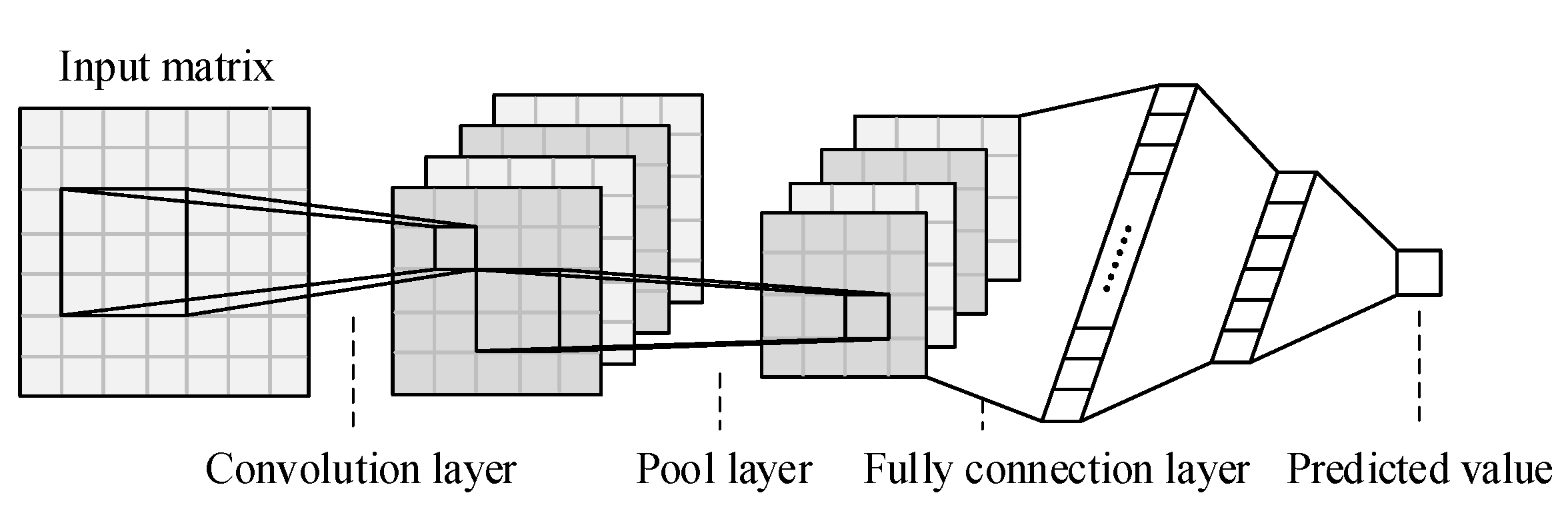
CNN is a powerful feedforward neural network, which is good at extracting features from matrix data and has strong data mining ability. The structure diagram is shown in Figure 1, which includes input layer, convolution layer, pooling layer, fully connection layer and output layer. The convolution layer can be regarded as the process of extracting features from data sources, which generally requires multiple convolution structures to work together. Due to data after the convolution layer having larger dimensions, we use the pool layer to segment the feature, so as to reduce the size of the feature graph. Finally, the full connection layer combines the local features into the global features.

The operation of the model is divided into training process, verification process and test process, which correspond to the training set, verification set and test set, respectively. The total data set consisted of wind power data in the last two years. The training process is divided into two stages: the forward propagation of data and the backward propagation error. By calculating the error between the output value and the real one, the model parameters will be continuously modified based on the gradient descent method and the training process ends after certain iterations. The verification process is accompanied by the training process. After each iteration, the model calculates the accuracy of the verification set according to the current network parameters, and saves the best ones as the optimal model. In order to guarantee the validity of the experiment, the intersection between the test set and the first two sets is not allowed. In the prediction process, the test set data is imported into the optimal model and its output is the prediction value of the CNN model.

In this paper, the CNN model is a single output structure, using the recursive prediction method to achieve 16 points of continuous prediction. It means that the predicted value is inserted into the last part of the input matrix, and the data points in the front of the input matrix are removed, and the prediction $x_{n+1}$ to $x_{n+16}$ can be achieved. After a prediction period is completed, real value $\left[x_{n+1},x_{n+2}\cdots x_{n+\tau }\right]$ can be introduced after the rolling step $\tau$, and the input data of the model can be updated. The method of intraday prediction by introducing the real value through the rolling step is called rolling prediction.

In addition, model hyperparameter optimization is also an important step to establish the network. An effective hyperparameter adjustment algorithm can not only improve the prediction accuracy, but also save the operation cost. In all, the input matrix data source has a great influence on the accuracy of the algorithm, as well as the combination of the convolution layer and pooling layer. Therefore, this paper focuses on data preprocessing and network structure determination when CNN is applied.

3. Long-Term Law Prediction Based on Similar Days

All data sets in CNN are wind power matrices arranged in chronological order and the time span of input data should not be too large, which implies that the long-term law cannot be captured. In this paper, the generalized similar day long-term forecast is proposed to make up for this shortcoming, and all the historical data are deepened, so as to effectively capture the law of historical similar data. Divide all data set $\left\{x_1,x_2\cdots x_t\right\}$ into $\left\{D_1,D_2\cdots D_n\right\}$,$D_n=\left[x_{t-nd+1},x_{t-nd+2}\cdots x_{t-\left(n-1\right)d}\right]$, where $d =96$ is the total number of sampling points in a day. Then, the grouped and divided data are defined as the long-term data set, which are used to search for the generalized similar days. The rolling prediction method is also used in multi-step prediction.

3.1. Similar Day Search

The goal of looking for similar days is to find out the data closest to the trend of wind power on the day (base day) before the forecast day in all historical wind power data, and to use the trend of the next day to revise the forecast results, so as to improve the forecast accuracy. The similarity criteria are as follows:

Pearson correlation coefficient:

$${\rho }_{(\mathrm{X},\mathrm{Y})}=\frac{\mathrm{cov}\left(X,Y\right)}{{\sigma }_X{\sigma }_Y}=\frac{E\left[\left(X-{\mu }_X\right)\left(Y-{\mu }_Y\right)\right]}{{\sigma }_X{\sigma }_Y}$$

(3)

Cosine similarity:

$$\cos (X,Y)=\frac{{\displaystyle \sum _{i=1}^n{X}_i\times Y_i}}{\sqrt{{\displaystyle \sum _{i=1}^n{(X_i)}^2}}\times \sqrt{{\displaystyle \sum _{i=1}^n{(Y_i)}^2}}}$$

(4)

Combination similarity:

$$S_{(X,Y)}={\rho }_{(X,Y)}+\cos (X,Y)$$

(5)

where $X$ and $Y$ are the comparison day data and base day data, respectively.

On the basis of the single method, considering that the Pearson correlation coefficient (PCCs) and cosine similarity value interval are the same, we put these two methods together as the combination similarity day selection method. In the actual case, it is necessary to carry out multiple groups of comparative experiments on large-scale data, and the best calculation method can be determined to predict the test set to avoid data leakage.

3.2. Applicability Analysis of Similar Days

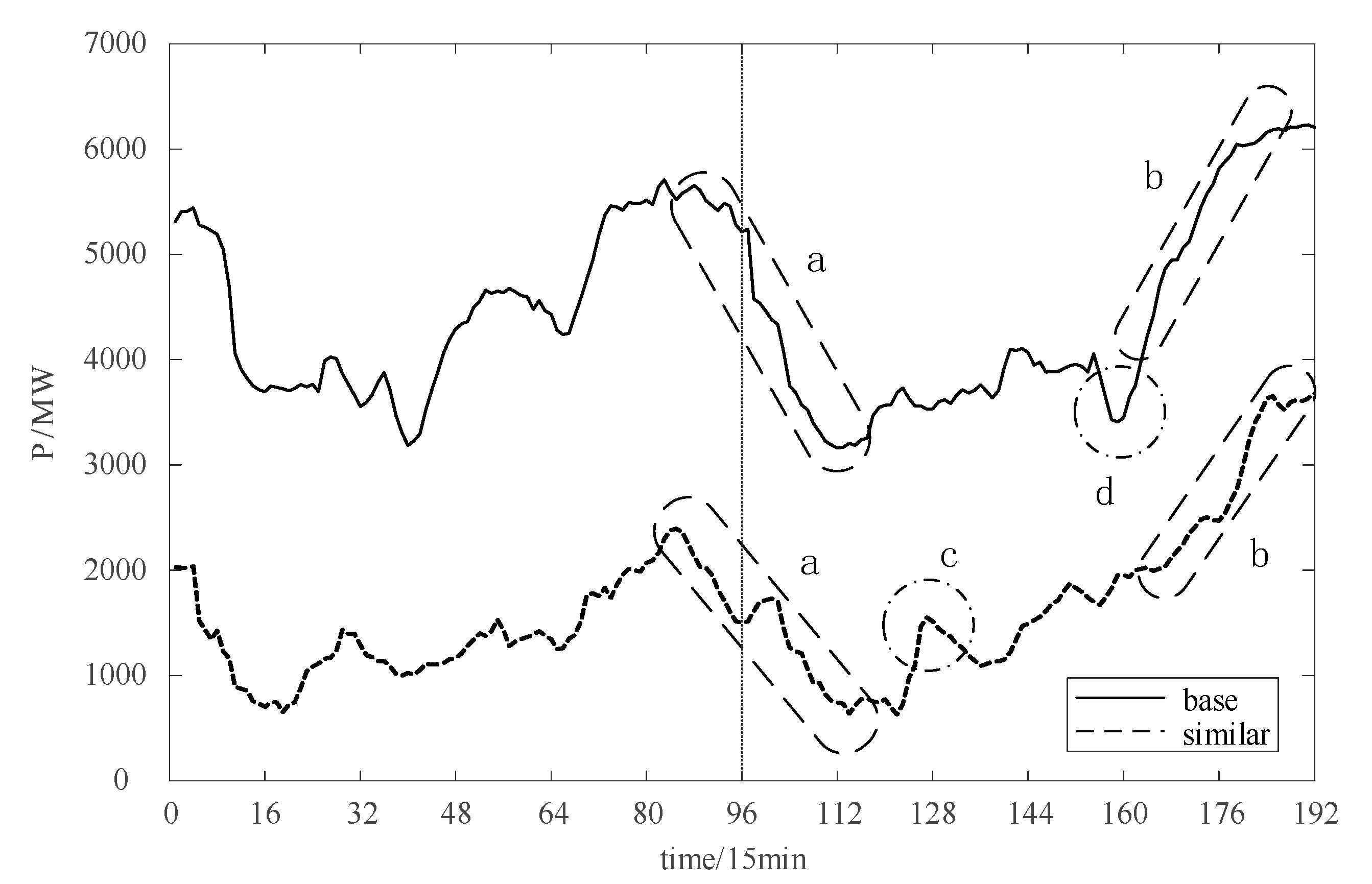
Similar days mainly take meteorological similarity into account, which means that there is still a certain correlation between the follow-up trends of similar data in the two historical periods. The trend comparison of similar days selected by Formula (5) on a base day is shown in Figure 2.

The solid line and dotted line on the left side of Figure 2 are the base day (2019-1-1) and similar day (2019-2-3), respectively, and the trends of these two in the next day are on the right side of the figure. It can be seen that the wind power of the next day in similar days tends to converge in the time interval of downhill (a), climbing (b) and stable period, and the trends have a high degree of correlation. While there are differences in the small peaks (c) and troughs (d), it can still be an effective aid for prediction.

4. Long Short-Term Combined Optimization Prediction

The operation principle of the short-term and long-term prediction model is described above, and the feasibility is analyzed. In some cases, the CNN model can predict well, but in other cases, the prediction accuracy of similar days is higher. In the actual prediction, we require the scientific and rigorous combination method to make the total statistical index optimal in a long time, since we cannot know the best combination weight in advance.

4.1. Select Combination Weighting Method

The combination weighting method can be divided into the subjective weighting method and objective weighting one, where the subjective weighting method is represented by the analytic hierarchy process (AHP). The weights are reasonably evaluated according to the decision-making problems and their own experience. However, the decision-making results are subjective and arbitrary, which means that it is difficult to provide effective and scientific weighting criteria in the wind power prediction problem. Due to these great limitations, this paper focuses on the objective weighting method.

The objective weighting methods for wind power prediction include the equal weight average method, time-varying weight method, entropy weight method, genetic algorithm and particle swarm optimization (PSO). Among them, particle swarm optimization is a random search algorithm based on group cooperation, which has strong global optimization search ability, fast convergence and high accuracy, and can effectively avoid falling into local optimization. The optimization process simulates the behavior of birds’ predation, where each particle is a possible solution of search space, and the particle dynamically adjusts the speed and direction of flight according to its historical optimal position and population optimal position. The optimal solution of a single particle search is called the individual extremum, and the optimal one in the particle swarm is called the global extremum. Through continuous iteration, the optimal solution satisfying the termination condition can be obtained.

In addition, the neural network is designed in several works for weight selection, which considerably increases the model complexity and time cost. Considered synthetically, particle swarm optimization is chosen in the experiment as the objective combination weighting method to avoid the subjectivity of artificial weighting or AHP.

4.2. Total Prediction Structure

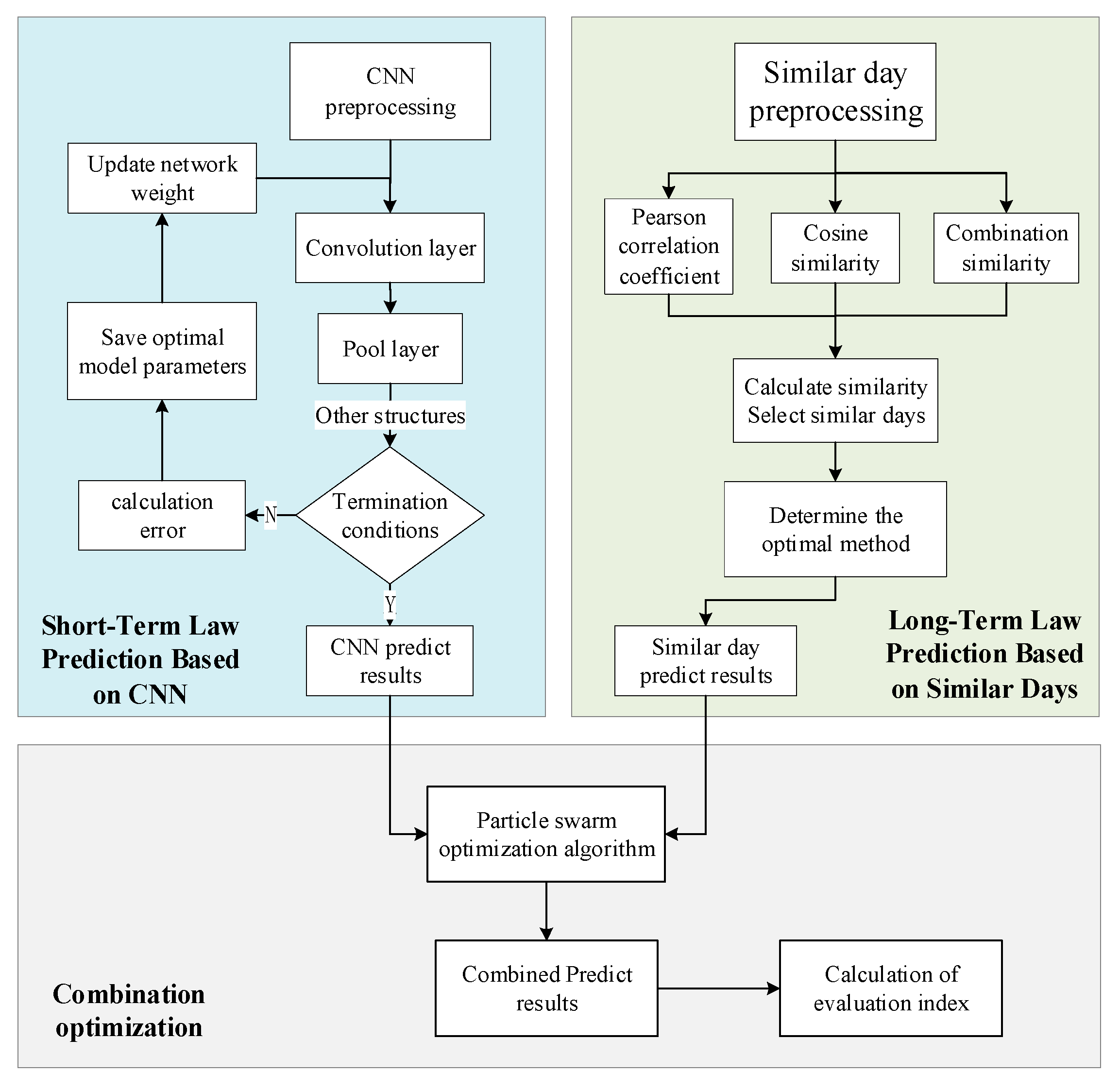
The general structure of the model is shown in Figure 3. On the left is the short-term law prediction model based on CNN. By using the verification set data, the optimal network structure can be achieved and then the base day data are input into the optimal CNN model, and the CNN predicted results can be obtained through recursive prediction. On the right is the long-term law prediction model of similar days. Similar to the CNN model, the optimal similar day selection algorithm is selected according to the verification set, and the candidate similar days are determined by calculating the similarity. Then, the PSO algorithm is used to determine the combination weight of the verification set, which is used to get the final predicted results.

In the CNN prediction process, we use the recursive prediction method above to forecast the data in the future period without introducing the true value, which belongs to multi-step prediction. After the prediction, the evaluation indexes of root mean square error ($RMSE$), percent error ($PE$) and qualified rate ($QR$) are used. The $PE$ indicator is similar to $RMSE$, which evaluates the error between the predicted value and the true value. The $QR$ indicator is closely related to power quality, because even if the average error is very low, a certain percentage of large errors will still threaten the operation of the power grid. Parameters $a$ and $b$ in $QR$ are determined according to the specific requirements of the power grid. The difference among them is that $RMSE$ reflects the absolute size of the prediction error, $PE$ reflects the relative value of the prediction error, and $QR$ reflects the compliance degree of the prediction results. Therefore, the predicted results can be evaluated comprehensively. The formulas for calculating the indicators are as follows:

$$RMSE=\sqrt{\frac{1}{m}{\displaystyle \sum _{i=1}^m{({\widehat{y}}_i-y_i)}^2}}$$

(6)

$$PE=\frac{1}{m}{\displaystyle \sum _{i=1}^m\left|\frac{{\widehat{y}}_i-y_i}{Z}\right|}$$

(7)

$$QR=\frac{1}{m}count\{\begin{array}{c}\begin{array}{cc}\left|{\widehat{y}}_i-y\right|\le ay+b& True\end{array}\hfill \\ \begin{array}{cc}else& False\end{array}\hfill \end{array}$$

(8)

where $m$ is the number of sampling points, $\widehat{y}$ and $y$ are the predicted value and the real value, $Z$ is the max power per day, $a$ and $b$ are adjustable parameters, determined by the actual dispatching situation of the power grid, and the proportion of $True$ is the qualification rate.

5. Case Analysis

Take the wind power data of a regional wind farm as an example. Specifically, there is a prediction system in the Beijing–Tianjin–Tangshan region of China where the maximum wind power is 7446 MW Through this prediction system, only the real data and predicted data of historical wind power in the last decade are sampled at a sampling frequency of 15 min. Ten years of data from 2010 to 2019 are used in similar day models for long-term law prediction, and the data of the last two years are used in the CNN model for short-term law prediction, so as to achieve the prediction goal of the next 4 h The feasibility of this method is verified by simulations, and the single CNN method, the single similar day method and the existing level (the prediction accuracy of this prediction system, which has been running for more than three years) are compared using three evaluation indexes to verify the superiority of the combined prediction method.

5.1. Select Combination Weighting Method

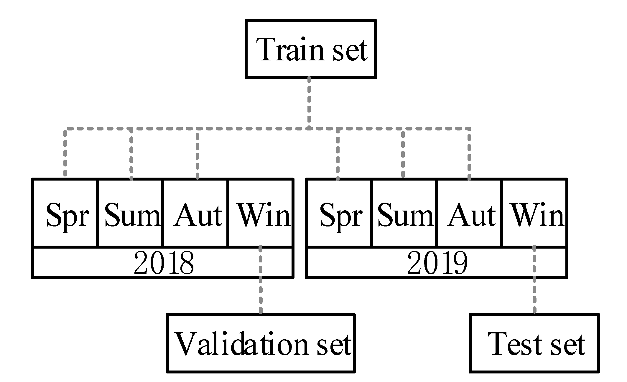
This paper selects the Tensorflow deep learning framework in Python to build the model. First, determine the $K$ value of the least square fitting. By testing the $K$ value in References [10,20], the optimal $K =15$ can be achieved. Then, normalize and matrix the fitted data with BN. Take the winter data of the year 2019 as an example, the CNN data set is divided as follows:

In the data set divided in Figure 4, considering the seasonal characteristics of wind power, the validation set is selected as the same quarter of the year before the test set. In the verification set, the method of grid optimization is used to optimize the super parameters of CNN. In the CNN training, a simple grid search method is used to traverse the value interval set by hyperparameters and selects the optimal hyperparameters without excessively increasing the complexity of the model. The structure and training parameters of the optimal CNN network are shown in

Table 1. CNN networks structure parameters.

Structure	Input Size	Conv Kernel/Filter
Conv1	8 × 8	4, (2 × 2)
Average Pool1	6 × 6	2 × 2
Conv2	3 × 3	16, (2 × 2)
Dense	128
Dense	64
Dense	1

and

Table 2. CNN training parameters.

Parameter	Value
Loss	Mean squared error
Optimizer	Adam
Epoch	90
Batch size	128

, respectively.

In addition, each layer of the CNN uses the relu activation function, and the steps of convolution kernel and pooling kernel are 1 and 2, respectively. In the end, the recursive prediction method is adopted to achieve 64 to 16 prediction structures.

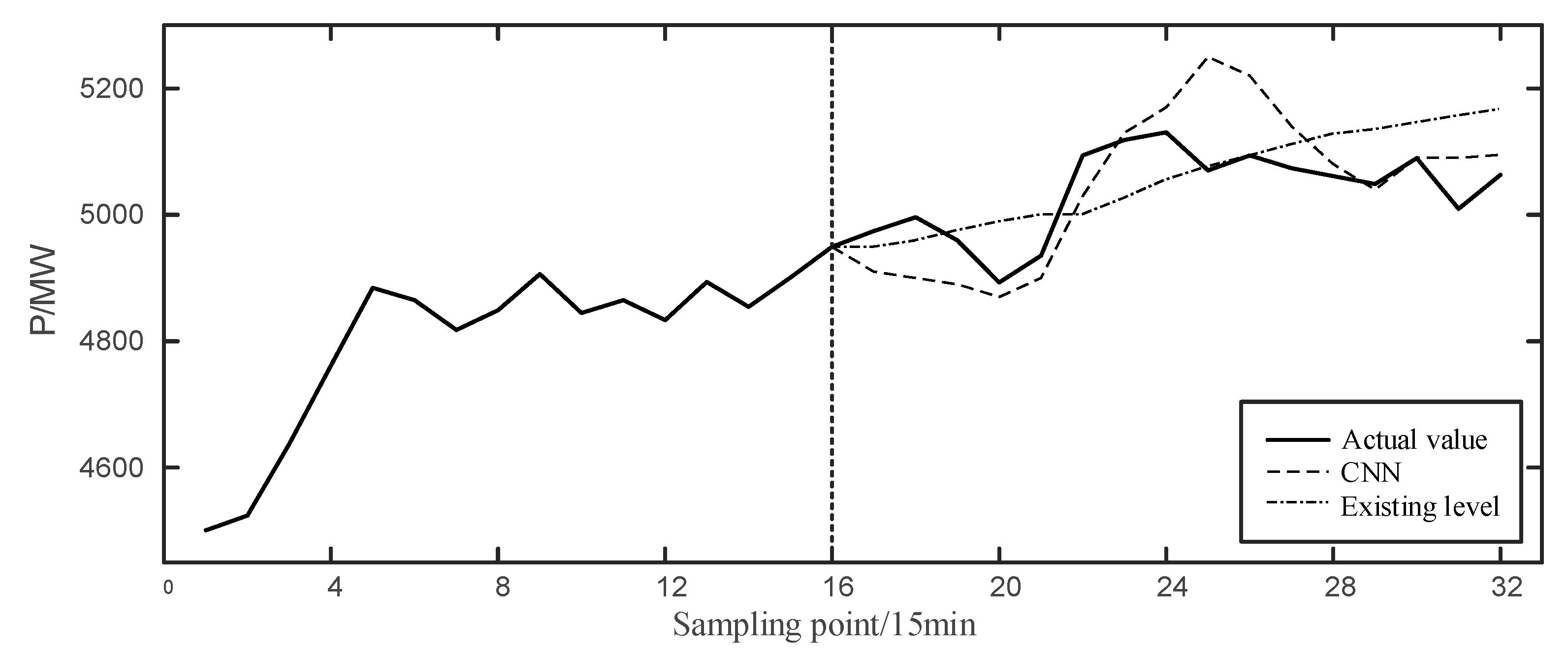
According to the prediction process of CNN in Figure 3, take the time interval 0:00–4:00 on 6 November 2019 as an example, and the predictive effect is as follows:

In Figure 5, the left side of the vertical dotted line is the actual curve at 20:00–24:00 on the previous day, and the right side is the effect comparison of the forecast curve. $RMSE$ and $PE$ indexes of CNN are 266.85 MW and 4.63%, respectively. It can be seen that the existing level can track the actual value on the general trend, but there is no response at the fluctuation, so it can only meet the basic forecast demand. CNN predicted results successfully predicted the time of the first trough, and followed the climbing process well. However, after the 24th point, it continued to rise and deviated from the actual curve until the 29th point. Yet the climbing response time is too long.

Generally speaking, CNN is more sensitive to the short-term data and has a good tracking effect. The farther it is from the prediction starting point, the more difficult it is to achieve accurate prediction. Thus, similar days need to be introduced to assist prediction, so as to improve the prediction accuracy.

5.2. Similar Day Forecast

In order to select the most suitable similar day, the similar day method in Section 2.1 is used as the validation set for prediction, and the prediction effect is shown in

Table 3. Statistical error of different similar days selection methods.

Method	PE
Euclidean distance	6.44%
PCCs	6.39%
Cosine similarity	6.36%
PCCs + Cosine similarity	6.31%

. It is shown that by using the combination of the Pearson correlation coefficient and cosine similarity, the prediction effect is the best. Therefore, this combination is selected to predict the test set data.

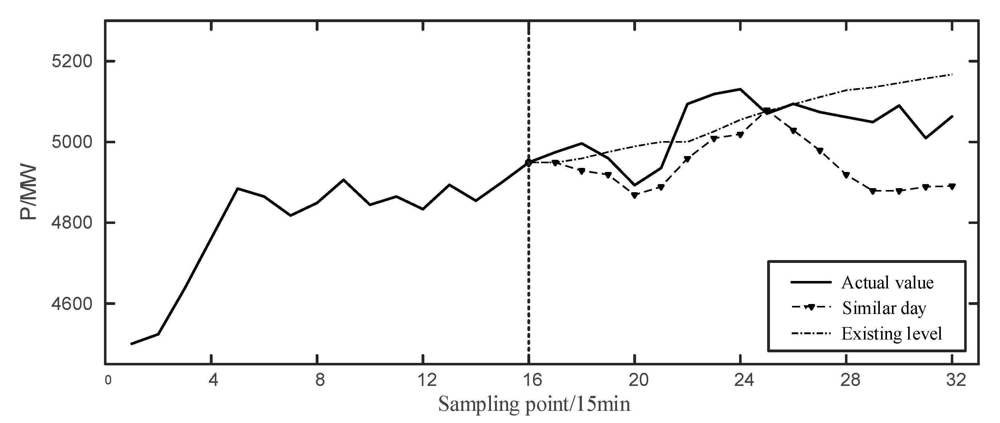
We also take the time interval 0:00–4:00 on 6 November 2019 as an example to conduct the prediction based on similar day, which is convenient for comparison between different models. The predicted results are calculated as follows:

In Figure 6, the prediction values of similar days are lower than the actual ones, but some inflexion points appear similar to the actual value. Moreover, the response of the similar days prediction at the wave crest is slow, and the downward trend in the second half is greater than the real situation, which can neutralize the long response of the CNN prediction.

5.3. PSO Combination Prediction and Error Analysis

The subsection tests the combination method mentioned above in the verification set, and the comparison results are shown in

Table 4. Statistical effect of combination weighting.

Method	CNN Weight	RMSE (MW)
Average weight	0.5	608.51
Time varying weight	change	620.91
Entropy weight method	0.474	607.43
Genetic algorithm	0.486	607.30
PSO	0.487	607.29

.

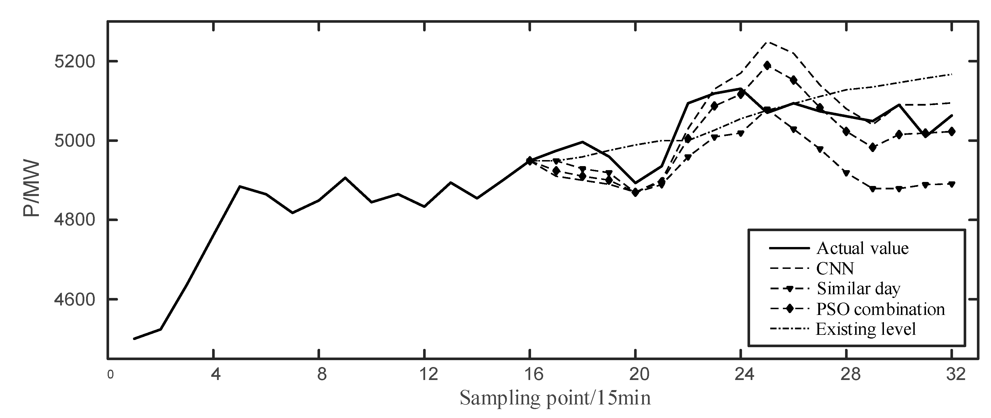
It shows that the RMSE of the combination weight determined by PSO is the smallest, and the predicted results of multiple models are shown as follows:

It can be seen from Figure 7 that the prediction curve using the PSO combination tracks the first trough well, corrects the response at the peak, fits the real value more closely, and the prediction accuracy is better than other individual predicted results.

To better verify this conclusion, statistical analysis is carried out on the whole year 2019, and the parameters $a$ and $b$ of the qualified rate in the evaluation index are taken 15% and 350 respectively. The annual prediction indexes are shown in the table below.

From

Table 5. Forecast indicators for the whole year of 2019.

Evaluation Indexes	CNN	Similar Days	Combination Model	Existing Level
RMSE (MW)	621.2	627.9	592.9	666.1
PE	6.07%	6.16%	5.79%	7.48%
QR	80.3%	78.6%	81.1%	71.0%

, we know that, compared to the existing level, $RMSE$ and $PE$ indexes of the combination model are reduced by 73.2 MW and 1.69%, respectively, and the corresponding $QR$ index is increased by 10.1%. Moreover, even if the CNN method and the similar days method can achieve higher prediction accuracy than the existing level, the prediction errors based on PSO weighting combination are the lowest, and the qualification rate is the highest at the same time. This is consistent with the theoretical analysis, that is, the combination model synthesizes the short-term laws (by CNN) and the long-term ones (by the similar days) to give a more accurate prediction. In a word, this method has a great application prospect to accurately predict the short-term wind power.

6. Conclusions

In this paper, based on the traditional CNN model, a new multi model combination forecasting method is implemented. The prediction accuracy is greatly improved compared to the existing level. The main contributions are as follows:

• On the basis of CNN′s wind power prediction, we add the prediction method of similar days, discuss its feasibility, make up for the shortcomings of the same time dimension of multi model combination prediction, and form the characteristics of CNN′s short-term law learning and similar days′ long-term law searching.
• In this paper, the PSO method is used to avoid the subjectivity in choosing combination weight. The result shows that the combined prediction algorithm of CNN and similar days with PSO has higher prediction accuracy and longer prediction period, which is an effective method.
• Regional wind power prediction is different from single base station prediction or single wind farm prediction. Regional wind power prediction is difficult to rely on real-time data or single regional meteorological data, and needs a longer time margin. Therefore, it requires fully mining the law in historical data to meet the prediction demand.