1. Introduction
Wind turbines control optimization is a major topic in the scientific literature about wind energy. Actually, the possible applications are impressive and widely impact on the practical wind farm operation as well as on the future perspectives of horizontal-axis wind turbines technology.
For example, it is remarkable that wind turbine control optimization can be conceived at the level of each single wind turbine or at the wind farm level. This work deals with the former type of approach; nevertheless it is important to recall that cooperative control [
1,
2,
3] and wake steering [
4,
5,
6,
7,
8] are two closely related aspects, currently standing at the frontier in the wind energy research: the objective is adopting non-trivial yaw and-or pitch control strategies [
9,
10], in order to optimize the power production and possibly mitigate mechanical loads at the level of wind farm.
It should be noticed as well that another line of research has been currently developing and it deals with the control optimization at the level of single wind turbine. The practical application of this kind of control design technology evolution is the power capture efficiency improvement for wind turbines operating since a certain number of years. Also as regards this field of intervention, the attention is focused on the management of the blade pitches and of the yaw.
The control and monitoring of blade pitches is fundamental, in order to prevent the wind turbine from being affected by rotor loads impacting severely on the residual useful lifetime (RUL). For this reason, therefore, there are several studies in the literature dealing with pitch imbalance detection [
11,
12,
13,
14,
15,
16]. Since the blade pitch management is the most common control of the torque of wind turbines, on one hand a pitch imbalance or an inappropriate control can be shown to affect considerably wind turbine performance [
17,
18]. On the other hand, blade pitch control optimization is an extremely promising direction for the power production upgrade of wind turbines. This has been addressed, for example, in [
19]: the blade pitch optimization is simulated and the impact on wind turbine performance is studied by means of a novel Kernel regression method.
The yaw behavior is a key issue as regards performance and mechanical aspects of wind turbines. For this reason, similarly to what happens as regards blade pitch, on one hand it is important to detect and correct yaw misalignment with respect to the wind direction; on the other hand it is important as well to design more advanced yaw control strategies for increasing the wind power capture. In [
20], operation data analysis is performed and the behavior of a wind turbine in yaw is classified through the formulation of a yaw index in relation to the power curve. In [
21], Computational Fluid Dynamics (CFD) simulations are performed in order to characterize the influence of yawed inflow conditions on wind turbine performance: a cosine law for the relation between yaw angle and power output reduction is proposed. In [
22], an equivalent wind speed model and a yaw error model are employed for estimating how much yaw misalignment affects wind turbine performance. It arises that an average misalignment of 10° can cause a power loss up to the 10%. This result provides a remarkable order of magnitude, justifying why the diagnosis of yaw misalignment is particularly important for wind turbine practitioners. The difficulty in achieving this objective is given by the fact that wind turbine cup anemometers are mounted on the nacelle and therefore behind the rotor: in [
23], it is discussed that the yaw control based on this kind of measurements can be non-optimal and can affect the performance up to 5%. Furthermore, the use of nacelle anemometers measurements for yaw misalignment detection can be prohibitive and for this reason LIDAR [
24] anemometers are often employed, despite for wind turbine owners the adoption of further sensors means paying a cost. Nevertheless, in [
25], it is shown that appropriate nacelle anemometer data analysis can be effective for the diagnosis of yaw misalignment.
The above matters of fact justify that the design of optimized yaw control strategies has been recently attracting a certain attention in the literature. For example, in [
26], it is discussed that the conventional way of estimating the direction of the incoming flow is by using transducers placed atop the nacelle and downwind of the rotor, while advanced upwind measurement techniques could diminish the yaw error and improve the power capture of wind turbines. In [
27], a new yaw control structure is designed, basing on a wind direction predictive model; simulations are performed and the results are compared against operation data of wind turbines adopting the state of the art in industrial yaw controls and it is supported that the proposed novel yaw control can diminish the yaw error. In [
28], two yaw control systems are designed (a direct measurement-based conventional logic control and a soft measurement-based advanced model predictive control) and a multi-objective Particle Swarm Optimization-based method is employed to optimize control parameters. Operation data of a 1.5 MW wind turbine are employed in order to estimate the possible power capture improvement provided by each of the two proposals. In [
29], a novel data driven yaw control algorithm synthesis method based on Reinforcement Learning is introduced and the potential power capture improvement is simulated under several wind speed scenarios using the TurbSim software.
The common ground of the above manuscripts is that, in each study, operation data of wind turbines are employed as a basis for simulating the potential power improvement provided by innovative yaw control strategies. The present study has instead a different point of view and fills a lack in the literature about this subject: in this work, actually, an improved yaw control strategy recently adopted in industrial wind farms is studied. Since operation data before and after the upgrade of the yaw control system for the wind turbine of interest are at disposal, this work is not about simulation of innovative yaw controls: it deals instead with the assessment of innovative yaw controls.
To the best of the authors knowledge, this study is the first of this kind as regards yaw control and in general is connected to some recent studies in the wind energy literature, dealing with the assessment of wind turbine power curve upgrades. Actually, since the wind is a stochastic source, this objective is challenging because it must necessarily be based on the comparison between the post-upgrade power production and a model of how much the wind turbine would have produced in the same conditions if the upgrade had not taken place.
Modeling the power output of a wind turbine with the necessary precision for this kind of objective is complex, because of the multivariate dependency on climate conditions and operation parameters, and this situation calls for devoted techniques that have been addressed in some recent studies. Chronologically, the first study is [
19]. Two test cases are addressed: vortex generators installation on wind turbine blades and pitch angle optimization. The former test case is addressed through operation data analysis and the latter is addressed through the simulation of operation data, basing on the logic of the pitch control system. A modification of the Kernel regression method is proposed for dealing with this kind of problems. Sideways, vortex generators, and more in general aerodynamic retrofitting of wind turbine blades, is one of the most important strategies for improving the power capture: see for example [
30,
31,
32,
33,
34,
35,
36,
37,
38,
39]. The impact of vortex generators installation on wind turbine power production is addressed also in [
40]: in that work, the same Kernel method of [
19] is adopted using ordinary wind turbine operation data (with, in general, sampling time of some minutes). The turning point of that study is that a much simpler method (the so-called side-by-side, based on the comparison, before and after the upgrade, of the difference between the power of the target upgraded wind turbine and the power of a reference wind turbine) can be successfully employed if the data set is particularly large: this is achieved by employing time-resolved operation data, with a sampling time of the order of the seconds. This side-by-side method has been conceptually generalized in [
41], where a combined aerodynamic and control upgrade is studied and the power of the wind turbine of interest is modeled through linear regression: the input variables for the model result to be operation parameters (power, blade pitches, rotor revolutions per minute and so on) of the nearby wind turbines and are selected among all the possible covariates at disposal through stepwise regression algorithm. A similar approach has been adopted also in [
42], while in [
43,
44] non-linear regression methods (like Artificial Neural Networks) are employed for assessment studies of wind turbine power curve upgrades.
On these grounds, the present study is devoted to the assessment of the yaw control optimization on a 2 MW wind turbine operating in southern Italy. A preliminary analysis of the operation data (conducted in
Section 2) indicates that the optimization is effective because the occurrence of considerably high yaw errors diminishes. The challenging point is the quantification of the power improvement: this practically consists of the necessity of a reliable model for the power of the wind turbine of interest. An ordinary linear regression (as in [
41], for example) is not effective for the test case of interest, because of the remarkably high mutual correlation between the possible covariates of the model: the objective is therefore achieved in this work through a Principal Component Regression (PCR) and the result of this study is that the yaw control optimization provides a production improvement of the order of the 1%. The method should be considered a distinctive part of the outcome of this study, because it can be successfully employed for control and monitoring purposes in wind energy applications, and it should be noticed that resolving with an acceptable precision a performance improvement of this order of magnitude is a complex task, because of the multivariate dependence of the power output of a wind turbine on atmospheric conditions and operating parameters.
Summarizing, the structure of the manuscript is as follows: in
Section 2, the test case wind farm and the data sets at disposal for the study are described.
Section 3 is devoted to the description of the methods. The results are collected and discussed in
Section 4.
Section 5 is devoted to the conclusions and the further direction.
2. The Test Case and the Data Set
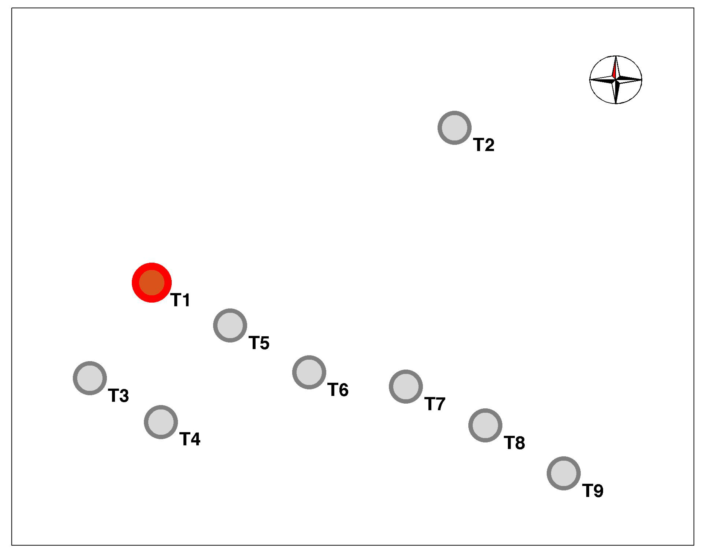
The layout of the wind farm is reported in
Figure 1 and in
Table 1 the inter-turbine distances are reported in units of the rotor diameter. The wind turbine of interest is T1 and is indicated in red in
Figure 1. The wind farm is composed of nine wind turbines sited in a flat terrain. The hub height is 80 m, the rotor diameter is 82.5 m, the cut-in wind speed is 3.5 m/s, the rated wind speed is 14.5 m/s and the cut-out wind speed is 25 m/s.
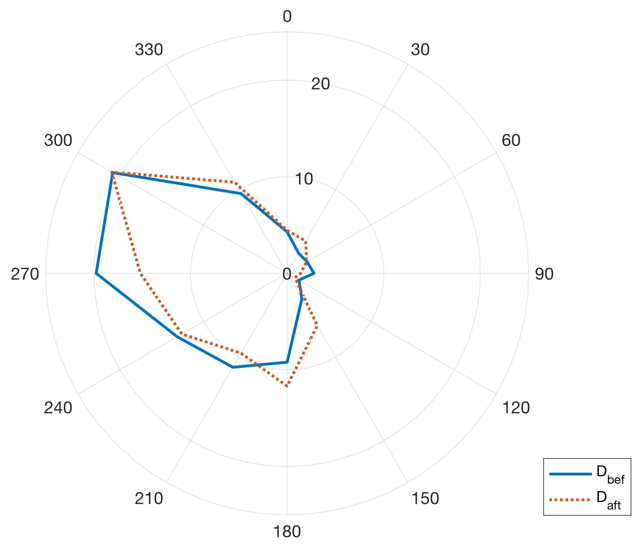
It should be noticed that several wind turbines are placed at around 4 rotor diameters with respect to their nearest ones: this indicates that potentially the wind farm is characterized by considerable wake interactions between wind turbines. The analysis of the wind rose (
Figure 2) actually indicates that this possibility is a matter of fact.
A long standing collaboration between the University of Perugia and the Renvico company (
www.renvicoenergy.com) has been established for wind turbine performance control and monitoring and for early fault diagnosis [
45,
46,
47,
48]. As regards the assessment of wind turbine power upgrades, the established framework is as follows:
one or more target wind turbines are selected for a pilot test;
the upgrade is installed on the selected wind turbine;
after some months of operation with the upgrade, the performance improvement is estimated through studies similar to the present one;
on the grounds of this estimate, a decision is taken about extending the upgrade installation to the rest of the wind farm or not.
Therefore, this study deals with the assessment of the pilot test and T1 has been the selected wind turbine, operating since a certain date with the improved yaw control. The selection of the pilot wind turbine for the power upgrade test can be based on several considerations. For example, one can point at testing the power upgrades at the wind turbines more affected by wakes, in order to estimate the improvement at the most disadvantaged wind turbines of the farm. On the other way round, one can test the upgrade at upstream isolated wind turbines, in order to estimate the impact of the upgrade when the working conditions of the pilot wind turbines are the best possible for the given wind farm. For the present test case, the decision has been a compromise between the two above considerations. Actually, it can be observed (
Figure 1) that the wind farm is composed of one isolated wind turbine and a compact cluster of eight wind turbines; in this cluster, the T6–T9 group is slightly disadvantaged because of multiple wake interactions when the wind blows from the 270° and 300° sectors (
Figure 2). Therefore, selecting T1 as pilot wind turbine means selecting a wind turbine from the main cluster, mostly operating upstream (
Figure 2).
The data at disposal have been consequently organized in two sets as follows:
The first data set is denoted as and contains the data collected from 1 March 2017 to 25 August 2018. It is a period prior to the intervention on turbine T1.
The second data set is denoted as and contains the data collected from 1 September 2018 to 1 March 2019. It is a period after the yaw control optimization on turbine T1.
The data have been filtered, using the appropriate counter available in the Supervisory Control And Data Acquisition (SCADA) system, on the request that each wind turbine in the wind farm has been productive. Upon data filtering, results to be composed of 31,755 measurements and is composed of 12,739 measurements.
The wind direction roses measured at T1 nacelle during
and
are reported in
Figure 2 and it arises that the wind direction distributions before and after the upgrade are remarkably similar. The ratio between the average nacelle wind speeds measured at T1 during
and
is 1.04.
The data have ten minutes of sampling time and the available validated measurements for each wind turbine in the wind farm are
nacelle wind direction;
power output;
ambient temperature;
nacelle position;
rotor speed;
generator speed;
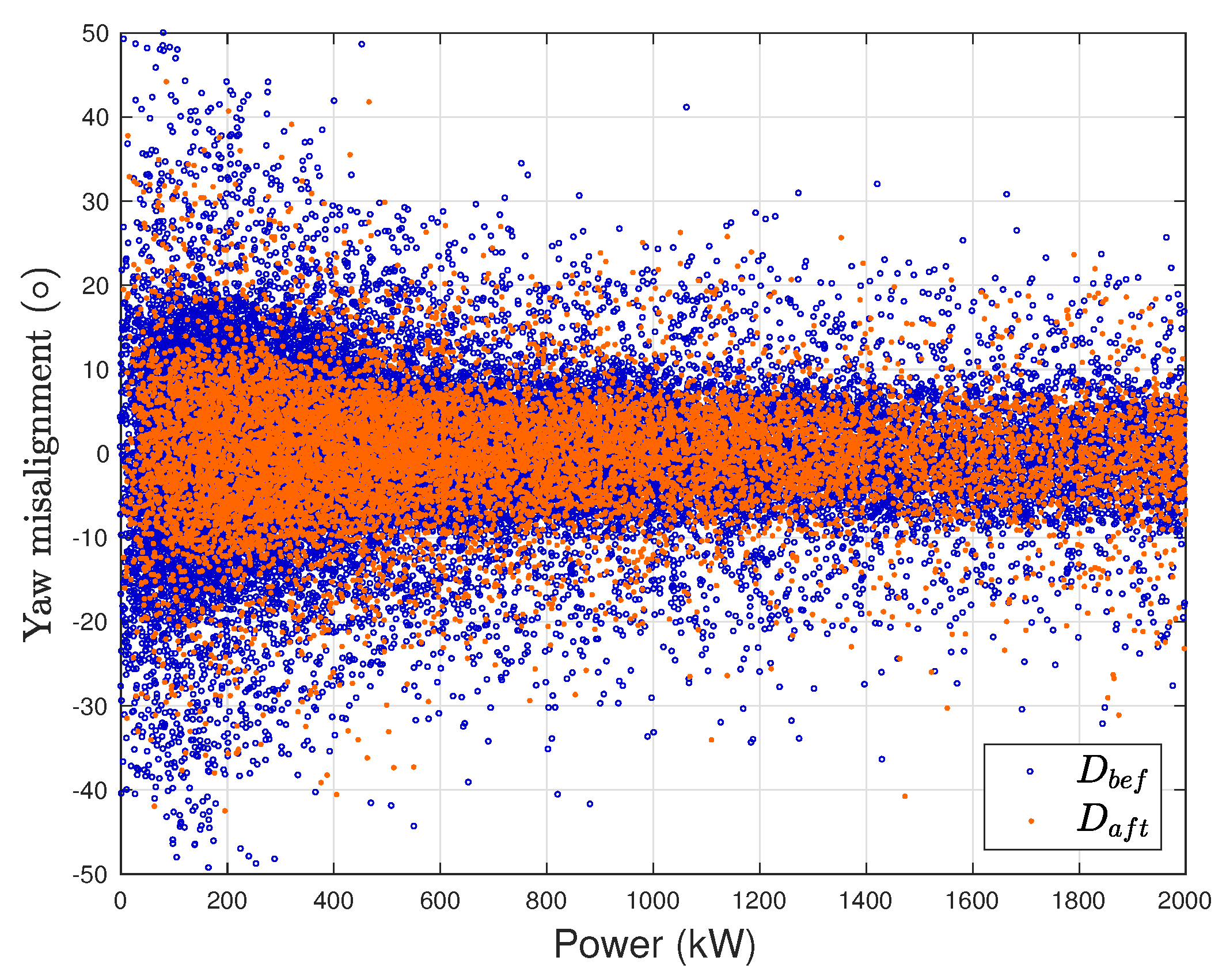
The yaw control upgrade considered in the present work consists of an optimization of the nacelle response when the yaw error exceeds a certain threshold. The net effect should be a decrease of the occurrence of high yaw errors and this implies an increase of the power production, because the power of a wind turbine depends on the yaw error with a cosine cube law [
22]. The dynamical improvement could be appreciable through the analysis of time-resolved data (with a sampling time of the order of the second); for the present study, operation data with ten minutes of sampling time were at disposal and the yaw upgrade effect reasonably can be detected only by a statistical point of view. Actually, from the nacelle wind direction and the nacelle position measurements, it is possible to estimate the yaw error as their difference. For wind turbine T1, the yaw misalignment as a function of the power is reported in
Figure 3 for data sets
and
. This plot provides a qualitative assessment of the fact that, after the upgrade of the yaw control, the frequency of considerably high yaw errors diminishes. A quantitative indication has been obtained by computing the frequency of absolute yaw errors higher than a threshold (10°): it arises that for T1, the frequency decreases from the 10% to the 6.2% from
and
. Consistently, this effect is not visible for the other wind turbines in the farm that have not been upgraded.
3. The Methods
The objective of this part of the work is formulating a reliable model for the power of the wind turbine of interest (T1). This is necessary because the estimate of the production upgrade (described in detail in
Section 4) basically consists of the comparison between the measured power after the upgrade and the model of how much the wind turbine would have produced under the same conditions if the upgrade had not taken place.
The idea for the model formulation is describing the on-site conditions through the ambient condition measurements at each wind turbine in the farm and through the operation variables of each wind turbine in the farm: all these quantities can in principle be input variables of the model for the power of T1 (denoted as
y in the following). This principle has been adopted, for example, in [
41] and in that work the variables selection for the model has been performed through a stepwise regression algorithm. The critical point as regards the application of that kind of regression for the present test case deals with the fact that some of the possible input variables are very highly correlated. This is due to the fact that the dynamics of the present wind farm is severely intertwined: the wind farm is sited in flat terrain and the layout is quite compact, differently with respect to the test case of [
41] (characterized by considerable altitude variations within a very vast wind farm layout). For example, the rotor speeds or blade pitches of nearby wind turbines in this test case wind farm can have a correlation coefficient up to 0.99 and this indicates that the multicollinearity problem must be addressed in the regression.
On these grounds, the Principal Component Regression (PCR) [
49] has been selected for this study: sideways, the use of this method for control and monitoring purposes in wind energy has been growing [
50]. The procedure goes as follows. Let
be the vector of measured output (namely the power of T1) and
be the matrix of covariatives.
n is the number of observations and
p is the number of covariatives. Notice that it might be appropriate that the
matrix has been rescaled and different possibilities are currently employed: rescale each column of
with its standard deviation (with or without having translated the mean of each column to 0), or rescale overall the
matrix with its maximum. For this work, it has been observed that the results do not depend sensibly on the normalization of the
matrix but slightly lowest averages mean errors are obtained when the
is not normalized and therefore this choice has been pursued.
The ordinary least squares regression assumes that
where
are the regression coefficients that must be estimated from the input variables data matrix
and
are random errors. The ordinary least squares estimate of
is given by
The principal component estimate of
is obtained as follows. Let
be the singular value decomposition of
. This means that the columns of
and
are orthonormal sets of vectors denoting the left and right singular vectors of
and
is a diagonal matrix, whose elements are the singular values of
. This allows decomposing
as:
where
and
.
is the i-th principal component and is the i-th loading corresponding to the i-th principal value .
The Principal Component Regression assumes that a linear relation can be established between the transformed data matrix and the target . In other words, the Principal Component Regression can be viewed as an ordinary least squares regression between and .
The usefulness of the Principal Component Regression and its superiority with respect to ordinary least squares regression is that the decomposition in Equation (
4) indicates a sort of regularization scheme: namely the matrix
can be truncated including a desired number of principal components. This is particularly useful for addressing the problem of multicollinearity of covariates, because when two or more covariates are highly correlated,
tends to lose its full rank and this implies that
has some eigenvalues tending to 0. Truncating up to a certain number of principal components means regularizing the covariates matrix in order that it has full rank. It should be noticed that there are critical points also as regards the truncation [
49], because there are arguments supporting that the principal components associated with eigenvalues with low absolute value can carry meaningful information. Nevertheless, for the objectives of the present study it has verified that this is not the case and the decisive point is including at least a certain amount of principal components.
Finally, the principal component estimate of
is given as
where it is assumed that the matrices can be truncated to a desired number of columns, i.e., principal components.
The structure of the model for the test case of interest has been selected as follows. The output is the power of T1; the covariatives matrix has been selected to be composed of power, rotor speed, generator speed, nacelle position and ambient temperature at each wind turbine of the wind farm, except T1. This has been done because it is likely that the yaw control optimization at T1 changes the relation between operation parameters and power output: therefore, the operation parameters of T1 cannot be used as references for modeling the power of T1. Therefore, if one considers the data set, is a vector of 31,755 data and is a matrix with 31,755 rows and 40 columns (5 variables for 8 wind turbines).
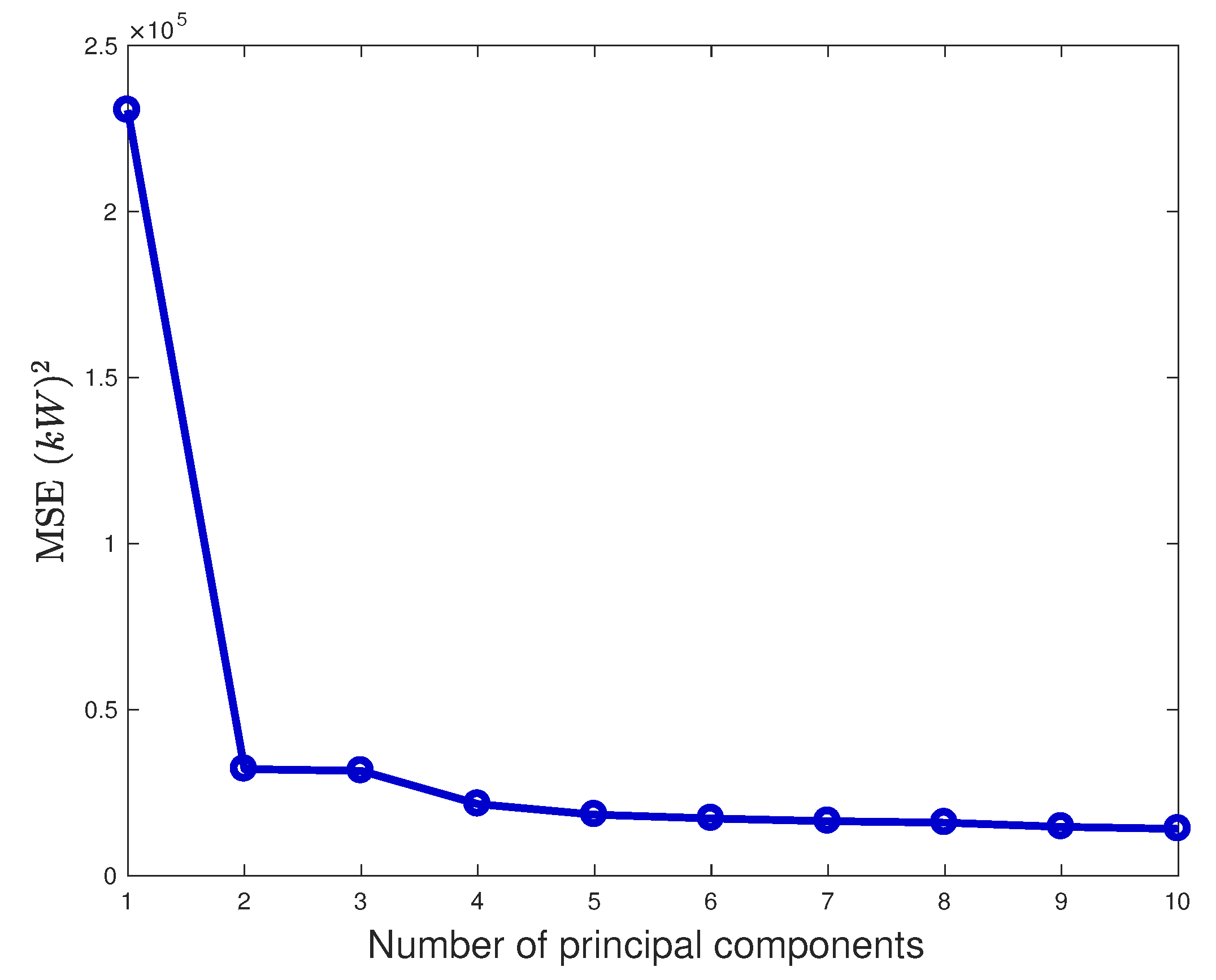
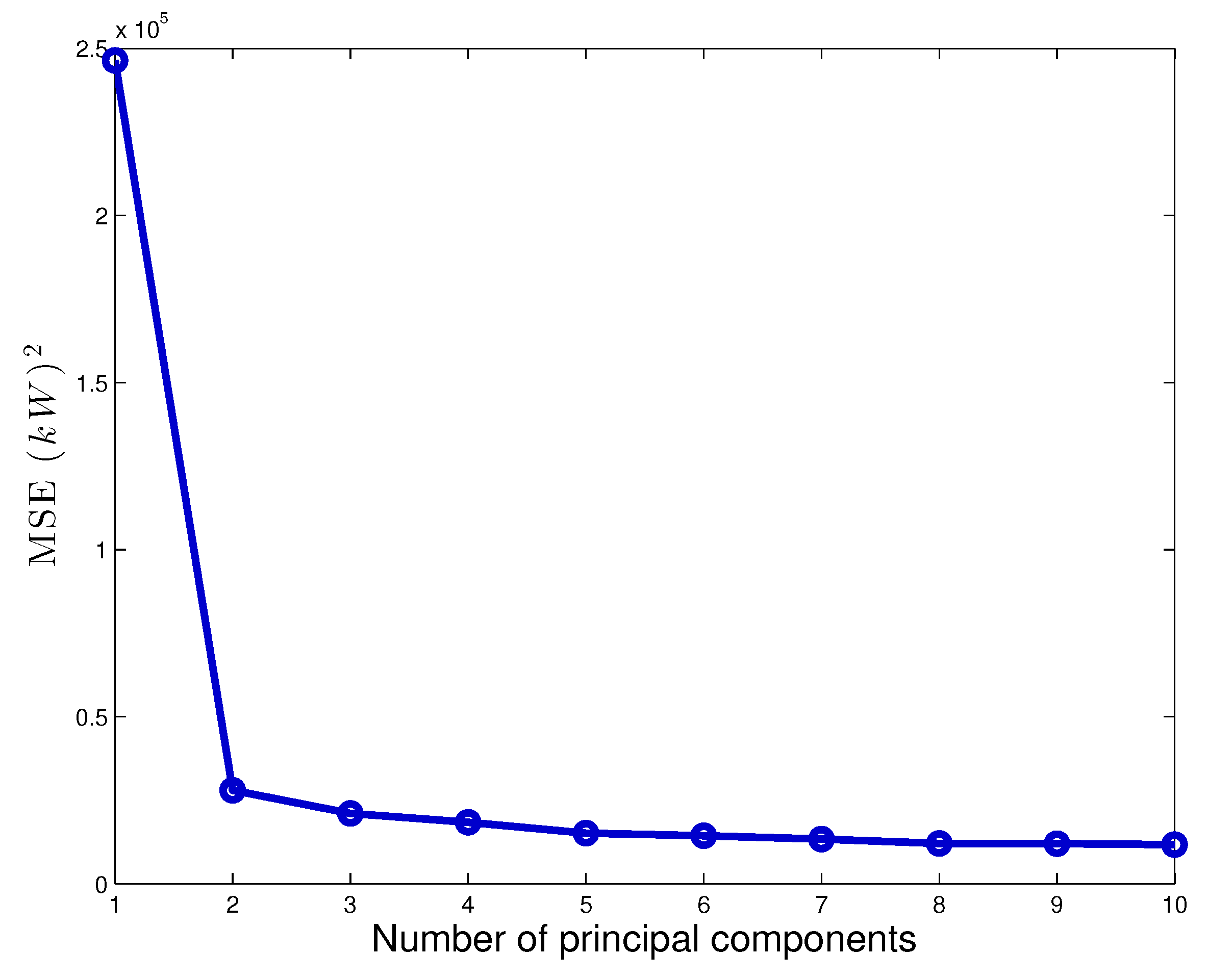
The selection of an adequate number of principal components for the regression is performed through
K-fold cross-validation [
51]. The procedure goes as follows: divide
randomly in two fractions, where
of the data are used for training and the remaining
are used for validation.
is selected for this study. The training data are therefore employed for estimating
through Principal Component Regression (Equation (
5)) and the model estimate of the validation data is given by
This procedure is repeated for each fold selection. The Mean Square Error (
) is selected for the estimating the regression error. It is defined as
where
is the number of observation of
. The
values are subsequently averaged on the folds selection and therefore, for a given number of principal components included in the regression, a unique metric for estimating the quality of the regression is obtained. The results for the
K-fold cross-validation are reported in
Figure 4 and it arises that, if the number of principal components is higher or equal than 5, the average
is basically stable. For this reason, 5 principal components have been selected for this study. A sensitivity analysis has been performed and it has been observed that the results do not change substantially by including more than 5 principal components.
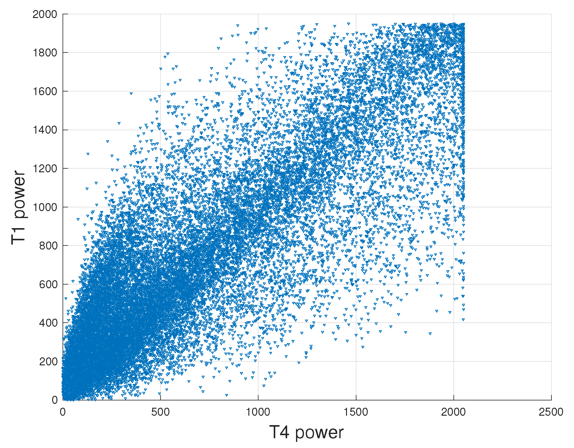
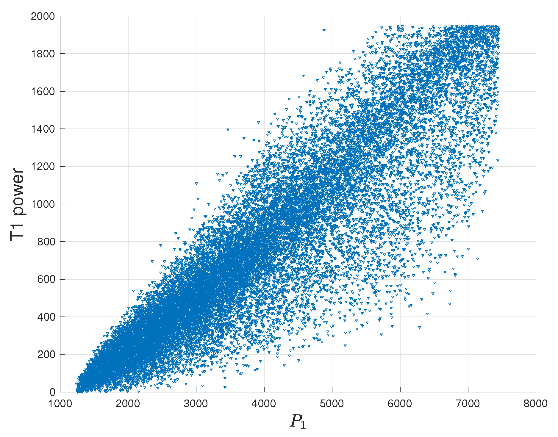
It is also possible to appreciate qualitatively how the principal component decomposition improves the quality of the regression. Consider the data set
: the target
y is plotted against the power of T4 (one of the covariatives having higher coefficient of determination
with respect to
y) in
Figure 5 and against the first principal component of the covariatives matrix in
Figure 6.
4. The Results
The data sets at disposal are employed as follows:
is randomly divided in two subsets: D0 ( of the data set) and D1 ( of the data set). D0 is used for training the model and constructing the weight matrix , D1 is used for validating the model.
(also named D2 for simplifying the notation in the following) is used to quantify the performance improvement.
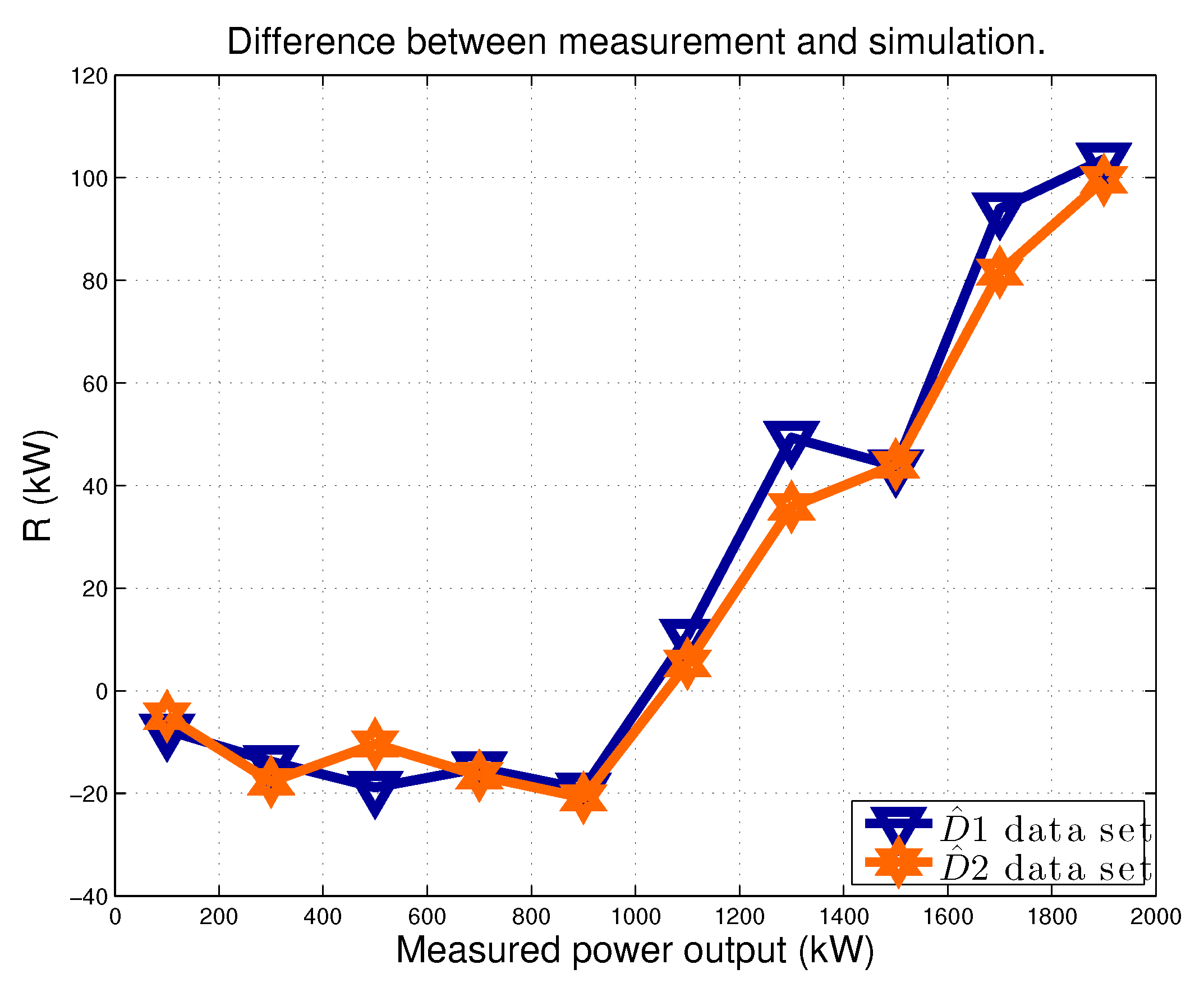
The upgrade can be estimated as a change in the behavior of the residuals for the D2 data set, with respect to D1. This should happen because the model is trained with pre-upgrade data and is employed to simulate one pre-upgrade data set (D1) and one post-upgrade data set (D2). Namely, the residuals between measurements and model estimates should averagely be 0 for the data set D1, while they should be negligibly be higher than 0 for the data set D2 (because the measured power should be higher than the power simulated according to a model trained with the pre-upgrade behavior). In the following, the procedure is reported for verifying if this is the case (and with what statistical significance) and for quantifying the upgrade.
Therefore, consider Equation (
8) with
.
For
, one has that the mean residual is
and the mean absolute residual is
where
is the number of measurements in data sets D1 and D2 respectively.
Since the measured
y and estimated
powers have all the same time basis (ten minutes), the quantity
where
is a percentage estimate of the energy improvement provided by the yaw control upgrade.
The above procedure has been repeated several times, by varying the random selection of D0 (and consequently of D1). The repetitions have been performed until the standard deviation of the
estimates (obtained for the different runs of the procedure) has become stable: as a rule of thumb, it can be said that 30 repetitions are sufficient. For each of these 30 runs of the model,
,
and
have been computed: these values have been averaged over the model runs and are reported in
Table 2 with a subscript indicating that they are the averages.
From
Table 2, it arises that the upgrade can be detected as an average increase of 8 kW in the difference between measurements and model estimates. A further question can be posed: how much statistically significant is this difference? The answer can be obtained by performing a Student’s
t-test to inquire if there is any statistically significant change in the turbine output after the upgrade. The
t-statistic is computed as
In Equation (
13),
and
are the numbers of data in, respectively, D1 and D2;
and
are the average residuals in data sets D1 and D2 respectively;
is given in Equation (
14):
where
and
are the standard deviations of the residuals in data sets D1 and D2 respectively. The
t-statistic (Equation (
13)) is computed to be of the order of
and this indicates that the probability that the upgrade is non-effective and that the observed difference in the residuals is given by random data picking within the same statistical ensemble is correspondingly low.
The average energy improvement is computed to be . In other words, the estimate is that, since the yaw control of T1 has been optimized, T1 has produced the more than it would have done if the upgrade had not taken place. The standard deviation is computed as and therefore the result can be presented as
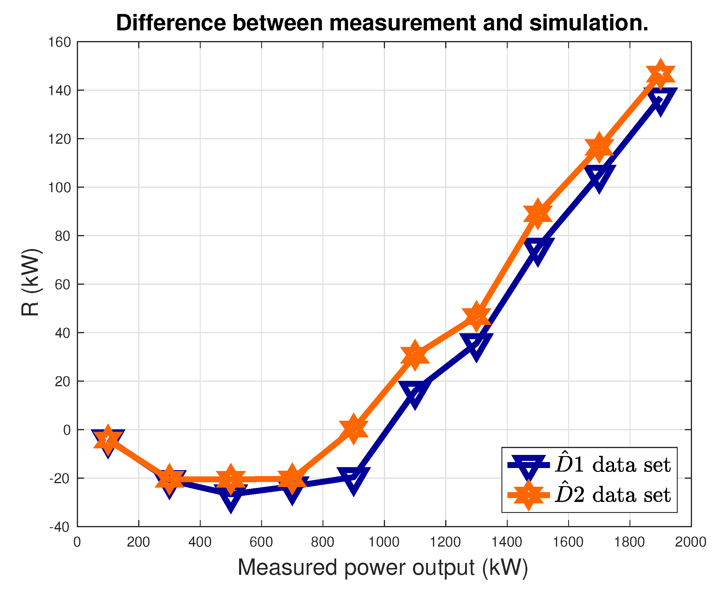
Finally, in order to appreciate how the yaw control upgrade changes the power production, it is possible to report a plot like the one in
Figure 7:
and
, computed on a sample model run, are displayed. The data are averaged in power production intervals, whose amplitude is 10% of the rated.
A Crosscheck of the Results
The reliability of the proposed method and of the results for T1 have been crosschecked by repeating the procedure for a wind turbine that has not undergone the yaw control optimization. In this case, actually, the performance improvement should consistently be estimated to be vanishing. T9 has been selected for this test. Therefore, the output
y for the model is the power of T9 and the covariatives matrix is composed of the variables listed in
Section 2 of the wind turbines T2 to T8. T9 operation variables are excluded from the possible covariatives, as is done in
Section 3 for T1, and the operation variables of T1 are excluded because they will have changed after the yaw control upgrade.
The results of the
K-fold cross-validation procedure are reported in
Figure 8: on these grounds, the decision has been employing 5 principal components but it should be noticed that the results do not change sensibly when including more than 5.
The results for the performance assessment are reported in
Table 3 and
Figure 9. The main indication is that the average difference between model estimate and power measurements changes of only 1 kW, while for T1 the average variation is 8 kW (
Table 2). From Equations (
11) and (12), one obtains
. The
t-statistic (Equation (
13)) is computed to be 0.4 and therefore the hypothesis that the performance of T9 during
and
come from the same statistical ensemble can not be rejected.
These results indicate, consistently, that the performance of T1 has changed after the upgrade and this can be detected with the proposed models with statistical significance; on the other way round, it can be detected with statistical significance that a non-upgraded wind turbine has performance compatible with the hypothesis that the performance has not changed.
5. Conclusions
This study has dealt with the assessment of wind turbine yaw control optimization through the analysis of operation data. As discussed in
Section 1, yaw control optimization is a topic that has been recently attracting a certain attention. The available studies in the literature mainly deal with the design of novel yaw control strategies and the simulation of the possible production improvement. This work instead fills a lack in the literature because the point of view is different. The test case is a 2 MW wind turbine operating in a wind farm composed of 9 wind turbines totally: the wind turbine of interest has undergone a yaw control optimization (diminishing the frequency of remarkably high yaw errors, as can be qualitatively appreciated from
Figure 3) and operation data before and after the intervention have been at disposal for this study. Therefore, the main objective of this work was the assessment of one yaw control optimization implemented in operating wind farms for industrial use. The assessment of this kind of control optimizations (and, in general, of wind turbine power curve upgrades) is interesting on its own, but it is further motivated by the fact that the efficiency of power upgrades can depend remarkably on the flow and on the on-site wind farm conditions.
The objective of this work practically translates in the formulation of a reliable data driven model for the power of the wind turbine of interest. This happens because the simplest way for assessing a wind turbine power upgrade is comparing the post-upgrade power production against a model of how much the wind turbine would have produced if the upgrade had not taken place. Particular attention has therefore been devoted to the formulation of an appropriate model for the power of the test case wind turbine. The underlying principle has been the use of the operation parameters of the nearby wind turbines in the farm as references for describing the on-site conditions.
Due to the remarkable multicollinearity of the possible model covariatives, a Principal Component Regression has been considered to be an adequate type of model. As regards the present test case, it has been observed that 5 principal components can be sufficient for modeling the power of the wind turbine of interest. Using this kind of model, it has been estimated that the wind turbine has its improved its power production of the 1% after the yaw control optimization. Sideways, this estimate is compatible with the available studies in the literature, indicating the rule of thumb that the impact of wind turbine control upgrades is of the order of the 1% of the annual energy production. A crosscheck of the results has also been proposed, by adopting the same kind of method for performance monitoring on a non-upgraded wind turbine and the obtained results are consistent.
Summarizing, these results support that the yaw is an important topic as regards the design of innovative wind turbine controls. Furthermore, these results should encourage wind turbine practitioners in the adoption of the most innovative wind turbine control strategies that are at disposal in the industry.
There are several possible further directions of the present work. One possibility is evidently the study of other test cases, in particular about yaw and in general about wind turbine control optimization. Another possibility is the adoption of more powerful information sources, as for example time-resolved data (as done for example in [
40]) because this would also allow appreciating the dynamics of the actual improved control strategies. A more general development regards instead the adopted methodology because, as discussed for example in [
50,
52], Principal Component Regression can be particularly useful for control and monitoring wind energy applications, dealing for example with advanced performance analysis, fatigue load analysis, early fault diagnosis.


