An Empirical Investigation on a Multiple Filters-Based Approach for Remaining Useful Life Prediction


Abstract
:1. Introduction
2. Backgrounds
Traditional Single-Filtering Approaches
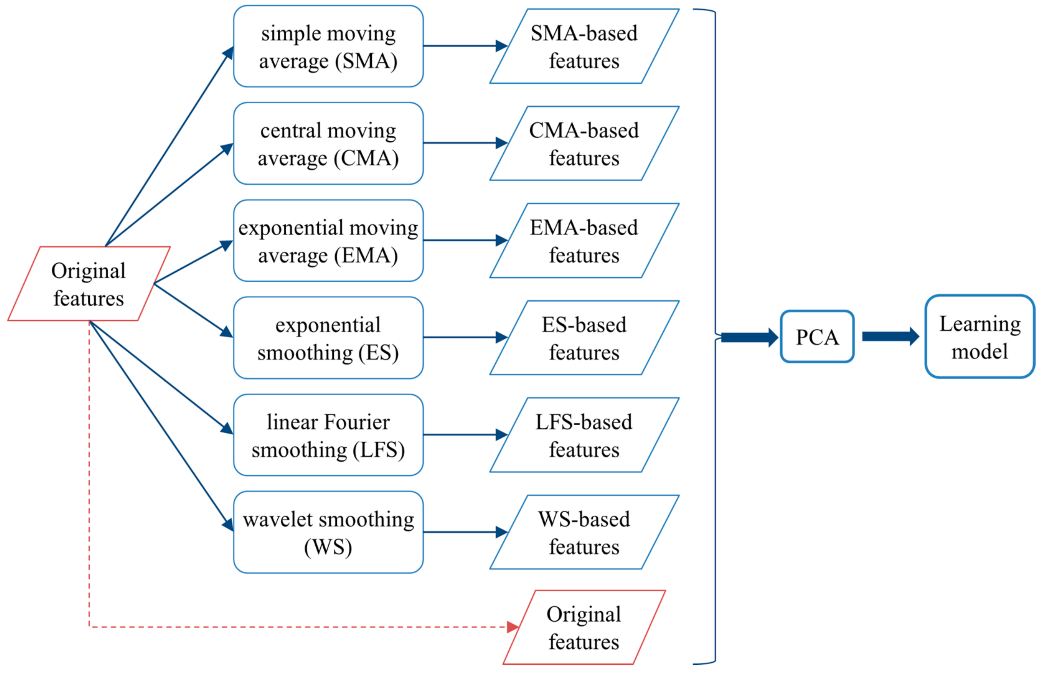
3. Our Proposed Approach
3.1. The Framework
3.2. Performance Evaluation Metrics
3.2.1. Scoring Function
3.2.2. Mean Squared Error (MSE)
4. Results and Discussion
4.1. Datasets
4.1.1. IEEE PHM 2012 Prognostic Challenge Dataset
4.1.2. NASA C-MAPSS Dataset
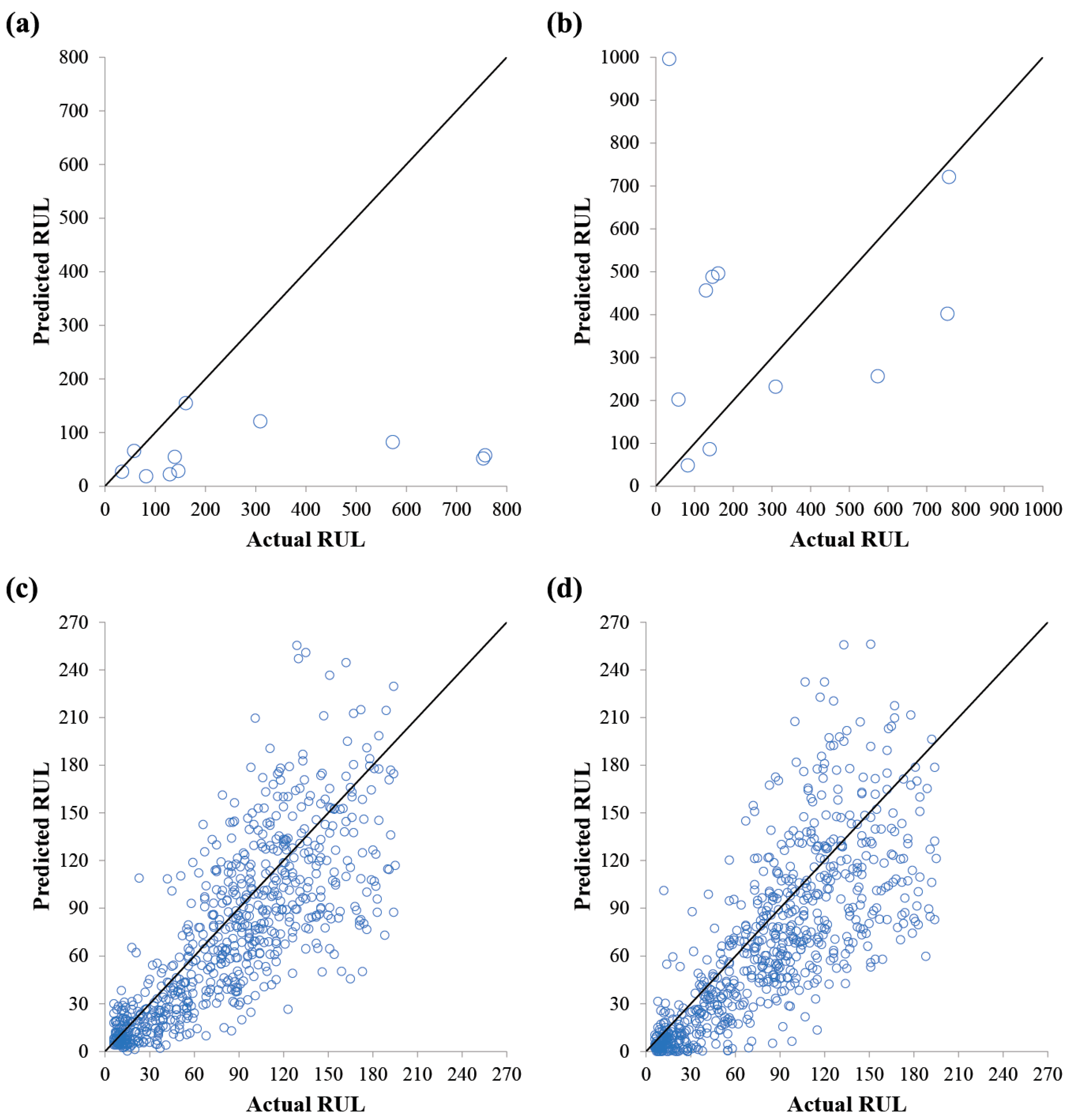
4.2. Performance Comparisons Between MF-PCA and SF-PCA
4.3. The Number of Components Selected by PCA
5. Conclusions
Author Contributions
Funding
Conflicts of Interest
References
- Sharp, M.E. Prognostic Approaches Using Transient Monitoring Methods. Ph.D. Thesis, University of Tennessee, Tennessee, TN, USA, 2012. [Google Scholar]
- Yu, M.; Wang, D.; Luo, M. Model-based prognosis for hybrid systems with mode-dependent degradation behaviors. IEEE Trans. Ind Electron. 2014, 61, 546–554. [Google Scholar] [CrossRef]
- Biswas, S.S.; Srivastava, A.K.; Whitehead, D. A real-time data-driven algorithm for health diagnosis and prognosis of a circuit breaker trip assembly. IEEE Trans. Ind. Electron. 2015, 62, 3822–3831. [Google Scholar] [CrossRef]
- Wei, Z.; Meng, S.; Xiong, B.; Ji, D.; Tseng, K.J. Enhanced online model identification and state of charge estimation for lithium-ion battery with a fbcrls based observer. Appl. Energy 2016, 181, 332–341. [Google Scholar] [CrossRef]
- Wei, Z.; Bhattarai, A.; Zou, C.; Meng, S.; Lim, T.M.; Skyllas-Kazacos, M. Real-time monitoring of capacity loss for vanadium redox flow battery. J. Power Sour. 2018, 390, 261–269. [Google Scholar] [CrossRef]
- Wei, Z.; Li, X.; Xu, L.; Cheng, Y. Comparative study of computational intelligence approaches for nox reduction of coal-fired boiler. Energy 2013, 55, 683–692. [Google Scholar] [CrossRef]
- Marinai, L. Gas-Path Diagnostics and Prognostics for Aero-Engines Using Fuzzy Logic and Time Series Analysis. Ph.D. Thesis, Cranfield University, Bedford, UK, 2004. [Google Scholar]
- Niknam, S.A.; Kobza, J.; Hines, J.W. Techniques of trend analysis in degradation-based prognostics. Int. J. Adv. Manuf. Technol. 2017, 88, 2429–2441. [Google Scholar] [CrossRef]
- Xi, X.; Chen, M.; Zhou, D. Remaining useful life prediction for degradation processes with memory effects. IEEE Trans. Reliab. 2017, 66, 751–760. [Google Scholar] [CrossRef]
- Riad, A.; Elminir, H.; Elattar, H. Evaluation of neural networks in the subject of prognostics as compared to linear regression model. Int. J. Eng. Technol. 2010, 10, 52–58. [Google Scholar]
- Goebel, K.; Saha, B.; Saxena, A. A comparison of three data-driven techniques for prognostics. In Proceedings of the 62nd Meeting of the Society for Machinery Failure Prevention Technology, Virginia Beach, VA, USA, 6–8 April 2008; pp. 119–131. [Google Scholar]
- Sutrisno, E.; Oh, H.; Vasan, A.S.S.; Pecht, M. Estimation of remaining useful life of ball bearings using data driven methodologies. In Proceedings of the IEEE Conference on Prognostics and Health Management, Denver, CO, USA, 18–21 June 2012. [Google Scholar]
- Aye, S.A.; Heyns, P.S. An integrated gaussian process regression for prediction of remaining useful life of slow speed bearings based on acoustic emission. Mech. Syst. Signal Process. 2017, 84, 485–498. [Google Scholar] [CrossRef]
- Xu, Z.; Ji, Y.; Zhou, D. A new real-time reliability prediction method for dynamic systems based on on-line fault prediction. IEEE Trans. Reliab. 2009, 58, 523–538. [Google Scholar]
- Wang, T. Bearing life prediction based on vibration signals: A case study and lessons learned. In Proceedings of the IEEE Conference on Prognostics and Health Management, Denver, CO, USA, 18–21 June 2012. [Google Scholar]
- Jovanović, M.; Filipović, Z.; Stupar, S.; Simonović, A. An example of equipment subsystem for aircraft life extending model. In Proceedings of the 4th International Scientific Conference on Defensive Technology, Belgrade, Serbia, 6–7 October 2011. [Google Scholar]
- Christophersen, J.P.; Motloch, C.G.; Morrison, J.L.; Donnellan, I.B.; Morrison, W.H. Impedance noise identification for state-of-health prognostics. In Proceedings of the 43rd Power Sources Conference, Philadelphia, PA, USA, 7–10 July 2008. [Google Scholar]
- Tobon-Mejia, D.; Medjaher, K.; Zerhouni, N.; Tripot, G. Estimation of the remaining useful life by using wavelet packet decomposition and hmms. In Proceedings of the IEEE Aerospace Conference, Big Sky, MT, USA, 5–12 March 2011; pp. 1–10. [Google Scholar]
- Zhang, C.; He, Y.; Yuan, L.; Xiang, S.; Wang, J. Prognostics of lithium-ion batteries based on wavelet denoising and de-rvm. Comput. Intell. Neurosci. 2015, 2015, 14. [Google Scholar] [CrossRef] [PubMed]
- Nectoux, P.; Gouriveau, R.; Medjaher, K.; Ramasso, E.; Chebel-Morello, B.; Zerhouni, N.; Varnier, C. Pronostia: An experimental platform for bearings accelerated degradation tests. In Proceedings of the IEEE Conference on Prognostics and Health Management, Denver, CO, USA, 18–21 June 2012. [Google Scholar]
- Peel, L. Data driven prognostics using a kalman filter ensemble of neural network models. In Proceedings of the International Conference on Prognostics and Health Management, Denver, CO, USA, 6–9 October 2008. [Google Scholar]
- Chen, J.; Ma, C.; Song, D.; Xu, B. Failure prognosis of multiple uncertainty system based on kalman filter and its application to aircraft fuel system. Adv. Mech. Eng. 2016, 8. [Google Scholar] [CrossRef]
- Bouzidi, Z.; Terrissa, L.; Lahmadi, A.; Zerhouni, N.; Ayad, S. The performance measure of a data driven prognostic system: Application to an aircraft engine. In Proceedings of the 2017 4th International Conference on Control, Decision and Information Technologies (CoDIT), Barcelona, Spain, 5–7 April 2017; pp. 790–796. [Google Scholar]
- FEMTO-ST. IEEE PHM 2012 Data Challenge Dataset, Nasa Ames Prognostics Data Repository. Available online: https://ti.arc.nasa.gov/tech/dash/groups/pcoe/prognostic-data-repository/#femto (accessed on 20 July 2018).
- Saxena, A.; Goebel, K. Turbofan Engine Degradation Simulation Data Set, Nasa Ames Prognostics Data Repository. Available online: https://ti.arc.nasa.gov/tech/dash/groups/pcoe/prognostic-data-repository/#turbofan (accessed on 20 July 2018).
- Saxena, A.; Goebel, K.; Simon, D.; Eklund, N. Damage propagation modeling for aircraft engine run-to-failure simulation. In Proceedings of the International Conference on Prognostics and Health Management, Denver, CO, USA, 6–9 October 2008. [Google Scholar]
- Wang, T.; Jianbo, Y.; Siegel, D.; Lee, J. A similarity-based prognostics approach for remaining useful life estimation of engineered systems. In Proceedings of the International Conference on Prognostics and Health Management, Denver, CO, USA, 6–9 October 2008. [Google Scholar]
- Heimes, F.O. Recurrent neural networks for remaining useful life estimation. In Proceedings of the International Conference on Prognostics and Health Management, Denver, CO, USA, 6–9 October 2008. [Google Scholar]
- Boškoski, P.; Gašperin, M.; Petelin, D. Bearing fault prognostics based on signal complexity and gaussian process models. In Proceedings of the IEEE Conference on Prognostics and Health Management (PHM), Denver, CO, USA, 18–21 June 2012. [Google Scholar]


| Category | Index | Condition 1 | Condition 2 | Condition 3 |
|---|---|---|---|---|
| Training set | 1 | 2802 | 910 | 514 |
| 2 | 870 | 796 | 1636 | |
| Test set | 3 | 1801 | 1201 | 351 |
| 4 | 1138 | 611 | N/A | |
| 5 | 2301 | 2001 | N/A | |
| 6 | 2301 | 571 | N/A | |
| 7 | 1501 | 171 | N/A |
| Sub-Dataset | C-MAPSS | |||
|---|---|---|---|---|
| FD001 | FD002 | FD003 | FD004 | |
| Train trajectories | 100 | 260 | 100 | 248 |
| Test trajectories | 100 | 259 | 100 | 248 |
| No. of operational modes | 1 | 6 | 1 | 6 |
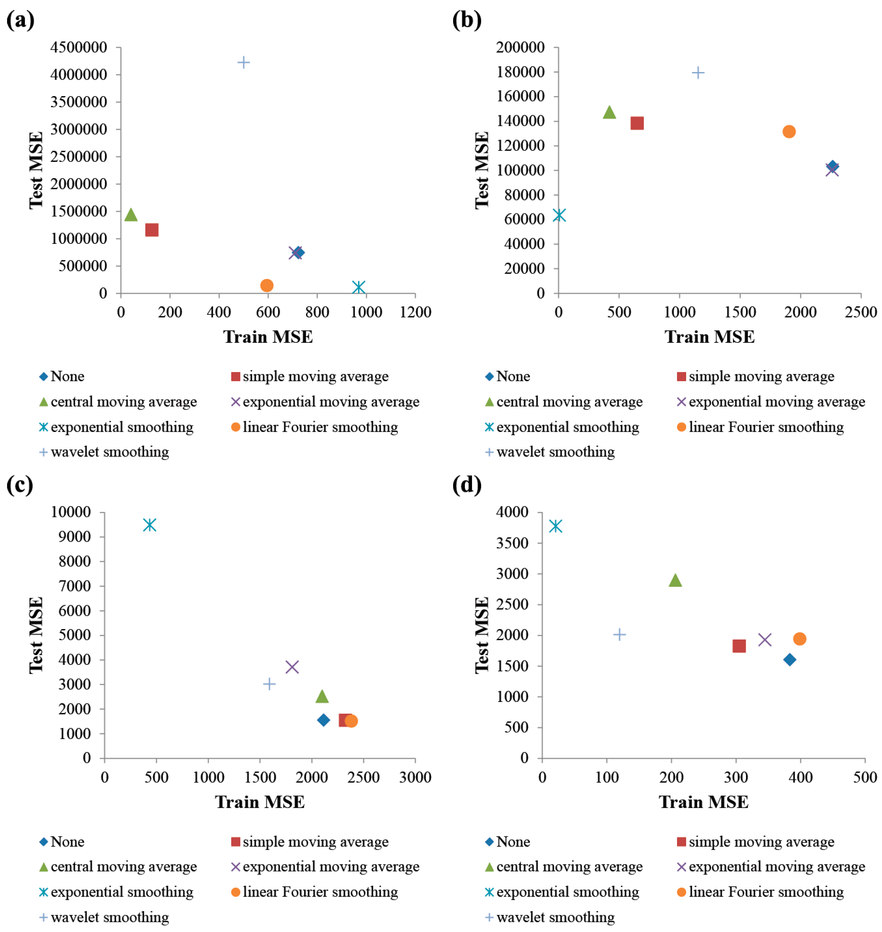
| (a) IEEE 2012 PHM Dataset | |||||||
| Filtering | MLP | RF | |||||
| Train MSE | Test MSE | Test Score | Train MSE | Test MSE | Test Score | ||
| None | 724 ± 103 | 744,198 ± 310,888 | 0.057 ± 0.033 | 2266 ± 137 | 103,123 ± 26,233 | 0.089 ± 0.044 | |
| Traditional SF-PCA | SMA | 127 ± 97 | 1,158,819 ± 403,550 | 0.076 ± 0.032 | 651 ± 83 | 138,249 ± 6789 | 0.152 ± 0.047 |
| CMA | 41 ± 16 | 1,439,890 ± 492,107 | 0.090 ± 0.041 | 421 ± 61 | 147,384 ± 10,721 | 0.116 ± 0.044 | |
| EMA | 711 ± 115 | 737,573 ± 295,667 | 0.049 ± 0.026 | 2261 ± 122 | 100,311 ± 24,294 | 0.083 ± 0.049 | |
| ES | 970 ± 2192 | 110,497 ± 19,777 | 0.095 ± 0.034 | 7 ± 2 | 63,471 ± 1919 | 0.118 ± 0.010 | |
| LFS | 595 ± 106 | 140,679 ± 110,303 | 0.100 ± 0.054 | 1906 ± 123 | 131,457 ± 13,699 | 0.128 ± 0.058 | |
| WS | 501 ± 430 | 4,225,192 ± 1,785,637 | 0.090 ± 0.032 | 1153 ± 106 | 179,486 ± 18,961 | 0.169 ± 0.037 | |
| MF-PCA | 2593 ± 3720 | 143,238 ± 37,597 | 0.113 ± 0.032 | 375 ± 41 | 107,308 ± 938 | 0.182 ± 0.017 | |
| (b) NASA C-MAPSS Dataset | |||||||
| Filtering | MLP | RF | |||||
| Train MSE | Test MSE | Test Score | Train MSE | Test MSE | Test Score | ||
| None | 2114 ± 757 | 1549 ± 320 | 0.258 ± 0.026 | 383 ± 158 | 1603 ± 315 | 0.250 ± 0.040 | |
| Traditional SF-PCA | SMA | 2326 ± 707 | 1543 ± 240 | 0.248 ± 0.028 | 305 ± 102 | 1823 ± 209 | 0.237 ± 0.026 |
| CMA | 2101 ± 684 | 2524 ± 1454 | 0.219 ± 0.077 | 206 ± 85 | 2897 ± 1530 | 0.203 ± 0.066 | |
| EMA | 1812 ± 896 | 3707 ± 2347 | 0.222 ± 0.017 | 345 ± 178 | 1926 ± 381 | 0.242 ± 0.038 | |
| ES | 436 ± 397 | 9485 ± 3210 | 0.095 ± 0.027 | 21 ± 20 | 3776 ± 1441 | 0.181 ± 0.033 | |
| LFS | 2383 ± 748 | 1512 ± 332 | 0.260 ± 0.018 | 399 ± 154 | 1941 ± 431 | 0.224 ± 0.024 | |
| WS | 1591 ± 465 | 3018 ± 1304 | 0.227 ± 0.035 | 120 ± 37 | 2011 ± 341 | 0.236 ± 0.020 | |
| MF-PCA | 1064 ± 799 | 1211 ± 243 | 0.291 ± 0.031 | 210 ± 166 | 1496 ± 264 | 0.265 ± 0.042 | |
| (a) IEEE 2012 PHM Dataset | |||||||||
| Filtering | NuOF | NuPC | |||||||
| Condition 1 | Condition 2 | Condition 3 | |||||||
| None | 768 | 435 | 436 | 338 | |||||
| Traditional SF-PCA | SMA | 397 | 388 | 340 | |||||
| CMA | 317 | 315 | 296 | ||||||
| EMA | 435 | 436 | 338 | ||||||
| ES | 125 | 134 | 123 | ||||||
| LFS | 449 | 445 | 349 | ||||||
| WS | 320 | 352 | 289 | ||||||
| MF-PCA | 5376 | 709 | 700 | 609 | |||||
| (b) NASA C-MAPSS Dataset | |||||||||
| Filtering | FD001 | FD002 | FD003 | FD004 | |||||
| NuOF | NuPC | NuOF | NuPC | NuOF | NuPC | NuOF | NuPC | ||
| None | 21 | 14 | 30 | 22 | 21 | 12 | 30 | 21 | |
| Traditional SF-PCA | SMA | 11 | 8 | 9 | 8 | ||||
| CMA | 10 | 9 | 8 | 8 | |||||
| EMA | 17 | 19 | 14 | 19 | |||||
| ES | 15 | 7 | 13 | 6 | |||||
| LFS | 15 | 9 | 13 | 8 | |||||
| WS | 5 | 14 | 7 | 14 | |||||
| MF-PCA | 147 | 50 | 210 | 41 | 147 | 39 | 210 | 38 | |
© 2018 by the authors. Licensee MDPI, Basel, Switzerland. This article is an open access article distributed under the terms and conditions of the Creative Commons Attribution (CC BY) license (http://creativecommons.org/licenses/by/4.0/).
Share and Cite
Trinh, H.-C.; Kwon, Y.-K. An Empirical Investigation on a Multiple Filters-Based Approach for Remaining Useful Life Prediction. Machines 2018, 6, 35. https://doi.org/10.3390/machines6030035
Trinh H-C, Kwon Y-K. An Empirical Investigation on a Multiple Filters-Based Approach for Remaining Useful Life Prediction. Machines. 2018; 6(3):35. https://doi.org/10.3390/machines6030035
Chicago/Turabian StyleTrinh, Hung-Cuong, and Yung-Keun Kwon. 2018. "An Empirical Investigation on a Multiple Filters-Based Approach for Remaining Useful Life Prediction" Machines 6, no. 3: 35. https://doi.org/10.3390/machines6030035
APA StyleTrinh, H.-C., & Kwon, Y.-K. (2018). An Empirical Investigation on a Multiple Filters-Based Approach for Remaining Useful Life Prediction. Machines, 6(3), 35. https://doi.org/10.3390/machines6030035