Adaptive Synchronization for Heterogeneous Multi-Agent Systems with Switching Topologies

Abstract

This work provides a multi-agent extension of output-feedback model reference adaptive control (MRAC), designed to synchronize a network of heterogeneous uncertain agents. The implementation of this scheme is based on multi-agent matching conditions. The practical advantage of the proposed MRAC is the possibility of handling the case of the unknown dynamics of the agents only by using the output and the control input of its neighbors. In addition, it is reasonable to consider the case when the communication topology is time-varying. In this work, the time-varying communication leads to a switching control structure that depends on the number of the predecessor of the agents. By using the switching control structure to handle the time-varying topologies, we show that synchronization can be achieved. The multi-agent adaptive switching controller is first analyzed, and numerical simulations based on formation control of simplifier quadcopter dynamics are provided.

1. Introduction

Research on synchronization of multi-agent systems (MASs) is inspired by certain collective animal behaviors, such as fish schooling, bird flocking, and bug swarming. The mechanism behind these behaviors can be found in crucial technological areas such as spacecraft formation flying [1], cooperative adaptive cruise control (CACC) [2], autonomous warehouse vehicles [3], smart power grids [4], robotics swarms [5], and smart buildings [6].

Prior to an explanation of the theory of synchronization of MASs, it is useful to give a definition of “agent”. The term “agent” appears in multiple disciplines in engineering and science; therefore, the term has been continuously revised. According to [7], an agent consists of four basic elements: the sensor, the actuator, the information element, and the reasoning element. According to [8], agents can be divided into three main categories: human agents, hardware agents, and software agents. Depending on the task, the software agent can be broken down into information agents, cooperation agents, and transaction agents. Information plays a crucial role in MASs: In centralized schemes, agents have access to global information, while in distributed schemes only access to the information from a few neighbors is possible [9,10].

In general, the study of synchronization has the objective of finding the coupling gains and/or the network topology that guarantee that the synchronization state error or the synchronization output error converges asymptotically to zero. Initial research on synchronization has been focusing on networks of identical agents, e.g., [11]. However, it is well known that agents can have heterogeneous dynamics, which makes synchronization more challenging [12]. Fixed coupling gains among the identical and non-identical agents that stabilize the synchronization error and guarantee the desired performance were proposed in [13]. Due to large uncertainties in network systems and unknown parameters, many distributed adaptive approaches have been developed to synchronize the agents. The distributed adaptive synchronization of the unknown heterogeneous agents and bounded misjudgment error was discussed extensively in [14]. In that work, synchronization was reached by using an extended form of state feedback model reference adaptive control (MRAC). Another approach based on the passification method was adopted to synchronize unknown heterogeneous MASs in [15]. Hybrid dynamics in networks may arise from networked-induced constraints [16] or from switching topologies.

In practice, the topology is not fixed and tends to change each time. An appropriate network structure or topology to achieve synchronous behavior was discussed in [17]. By using the proposed control laws, the topology changes lead to a different controller structure. In order to prove the stability of the switched system, one can rely on multiple Lyapunov functions and the dwell time switching law [18]. Novel model reference adaptive laws for uncertain switched linear systems to guarantee asymptotic and bounded stability were discussed in [19,20]. An open question pertains to how output synchronization can be achieved for heterogeneous agents with unknown dynamics in the presence of possibly switching topologies, and this question motivates this work.

The main contribution here is an extended adaptive synchronization law based on output- feedback MRAC for heterogeneous agents with unknown linear dynamics. It is to be noticed that our controller does not need any global information of the network. A Lyapunov-based approach is derived analytically to show that error converges asymptotically to zero. To address switching topologies, a novel switching adaptive controller is proposed in case some neighbor’s measurements cannot be accessed. Finally, numerical simulations are performed on a representative test case inspired by formation control of quadrotors.

The article is organized as follows: Section 2 introduces multi-agent output-feedback synchronization based on the MRAC approach. Section 3 includes switching communication topologies that handle the communication loss between agents. Section 4 presents the simulation to validate theoretical findings. Finally, Section 5 provides conclusions and proposes directions for further research.

Notation: The directed graph $\mathbb{G}$ is a pair ($\mathcal{N},\mathcal{E}$), where $\mathcal{N}=\{n_1,n_2,\dots ,n_n\}$ is a set of nodes and $\mathcal{E}\subseteq \mathcal{N}\times \mathcal{N}$ is a set of edges. The edge’s weight is defined as $a_{n_i{n}_j}$, where $n_i\ne n_j$. The $\mathbb{R}$ represents the set of real numbers. The matrices are denoted by capital letters, e.g., P, and the notation $P=P^T>0$ indicates a symmetric positive definite matrix. The identity matrix of compatible dimensions is denoted by I, and diag $\{\dots \}$ represents a block-diagonal matrix. The function $sgn(•)$ takes the sign •. The vectors are denoted by small letters, e.g., x. A vector signal $x\in {\mathbb{R}}^n$ belongs to the ${\mathcal{L}}_2$ class; if ${\int }_0^t{\left|\right|x\left(\tau \right)\left|\right|}^{2}d\tau <\infty$, $\forall t>0$. A vector signal $x\in {\mathbb{R}}^n$ belongs to ${\mathcal{L}}_{\infty }$ class; if max $\left|\right|x\left(t\right)\left|\right|<\infty$, $\forall t>0$.

2. Output-Feedback MRAC

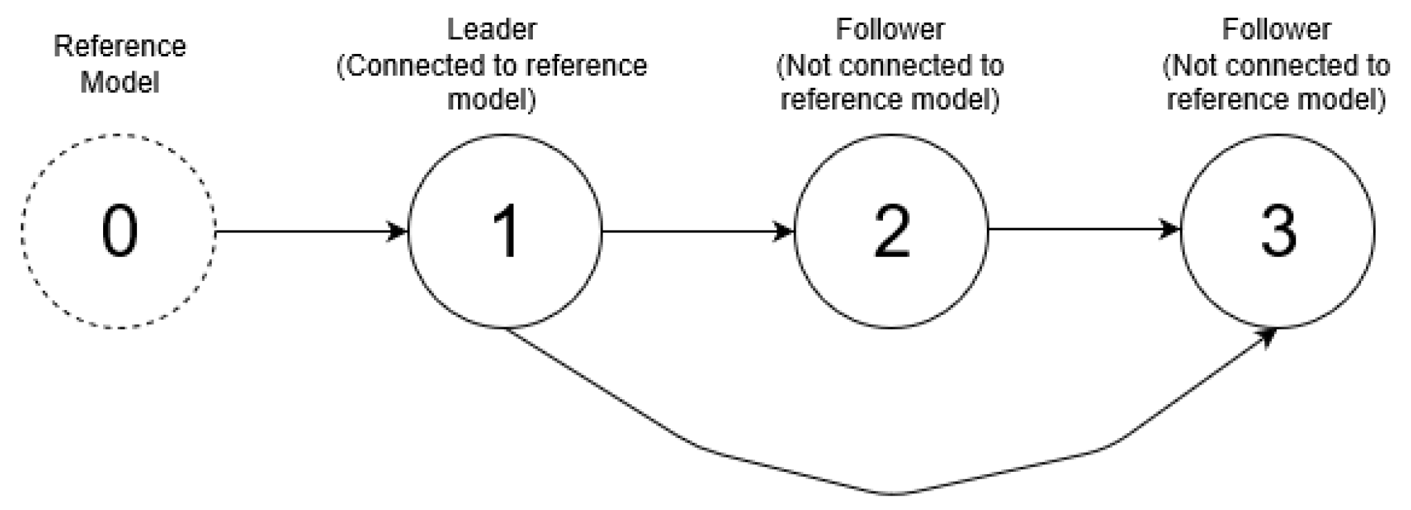
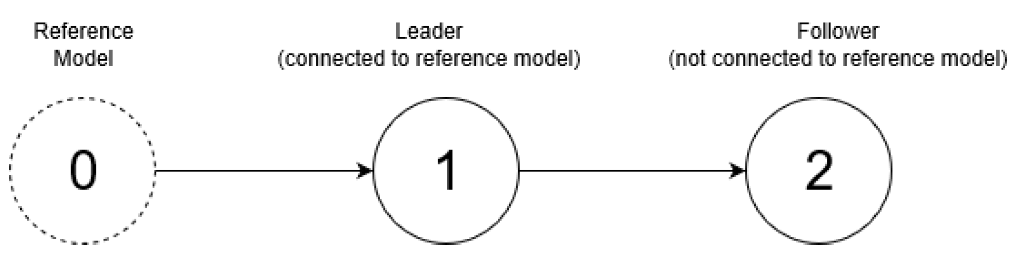
The main task in this section is to find the control laws $u_i\left(t\right)$ for each agent that guarantee synchronization of MASs with unknown linear dynamics by only using the input and the output of the neighbors. In order to facilitate the main result, let us assume that there are three agents denoted with subscripts 0, 1, and 2. Let us consider the network depicted in Figure 1. Here, the purpose of Agent 1, the leader, is to follow Agent 0. At the same time, the purpose of Agent 2 is to follow Agent 1. Agent 0 is a reference model that is connected to Agent 1, satisfying the following dynamics:

$$\begin{array}{cc}\hfill y_0& =G_0\left(s\right)=k_0\frac{Z_0\left(s\right)}{R_0\left(s\right)}r\hfill \end{array}$$

(1)

where $r\in \mathbb{R}$ and $y_0\in \mathbb{R}$ are the reference input and the output of the reference model. $Z_0\left(s\right)$ and $R_0\left(s\right)$ are known monic polynomials, and $k_0$ is the high-frequency gain. Next, we have Agents 1 and 2, denoted with subscripts 1 and 2, respectively, and with dynamics expressed in the transfer function form as

$$\begin{array}{c}\hfill y_1=G_1\left(s\right)=k_1\frac{Z_1\left(s\right)}{R_1\left(s\right)}{u}_1{y}_2=G_2\left(s\right)=k_2\frac{Z_2\left(s\right)}{R_2\left(s\right)}{u}_2\end{array}$$

(2)

where $u_1$,$u_2$$\in \mathbb{R}$, and $y_1$,$y_2$$\in \mathbb{R}$ are the inputs and the outputs of two agents. $Z_1\left(s\right)$, $Z_2\left(s\right)$, $R_1\left(s\right)$, and $R_2\left(s\right)$ are unknown monic polynomials, and $k_1$ and $k_2$ are constants referred to the high frequency gains. Note that, possibly, $Z_1\left(s\right)\ne Z_2\left(s\right)$ and $R_1\left(s\right)\ne R_2\left(s\right)$ (heterogeneous agents with unknown dynamics). We assume a directed connection from Agent 1 to Agent 2, i.e., the digraph is described by $\mathcal{N}=\{1,2\}$, $\mathcal{E}=\left\{\right(1,2\left)\right\}$. By using this configuration, Agent 2 can observe the measurement from Agent 1, but not vice versa.

The synchronization task between Agent 0 and Agent 1 is achieved when $y_1\to y_0$ for $t\to \infty$. As the signal from the reference model is known to Agent 1 only, the purpose of Agent 2 is to follow Agent 1. In this case, the synchronization task is achieved when $y_2\to y_1$ for $t\to \infty$. It is clear that, if both synchronization tasks are achieved, then we have also $y_2\to y_0$ for $t\to \infty$. These tasks should be achieved for any bounded reference signal r.

Assumption 1.

To achieve the synchronization objectives, we need the following assumptions for the reference model (R) and the agents (A):

(R1)

$Z_0\left(s\right)$ and $R_0\left(s\right)$ are monic Hurwitz polynomials, where the degree of $R_0\left(s\right)$ is less than or equal to the relative degree of $R_i\left(s\right)$, n.

(R2)

The relative degree of $G_0\left(s\right)$ is the same as that of $G_i\left(s\right)$, $i\in \{1,2\}$.

(A1)

$Z_i\left(s\right),i\in \{1,2\}$ are monic Hurwitz polynomials.

(A2)

An upper bound n of the degree $n_i$ of $R_i\left(s\right)$, i.e., $i\in \{1,2\}$, is known.

(A3)

The relative degree $n^{*}=n_i-m_i$ of $G_i\left(s\right)$, i.e., $i\in \{1,2\}$, is known, where m is the degree of the numerator. The relative degree of the agents and the reference should be the same.

(A4)

The sign of the high frequency gains $k_i$ i.e., $i\in \{1,2\}$ is known.

In the next subsection, the synchronization of Agent 1 to a reference model will be discussed.

2.1. Synchronization of a Leader to a Reference Model

As classical MRAC was used for the SISO plant in Chapter 5 of [21], it is well known that the agents i can be synchronized to the reference model by using the following control law:

$$u_i=l_1^{*T}\frac{\alpha \left(s\right)}{\Lambda \left(s\right)}{u}_i+f_1^{*T}\frac{\alpha \left(s\right)}{\Lambda \left(s\right)}{y}_i+g_1^{*}{y}_i+c_1^{*}r$$

(3)

where $\Lambda \left(s\right)$ is a Hurwitz monic polynomial and $\alpha$ are defined as

$$\begin{array}{cc}\alpha \left(s\right)\hfill & =\left[\begin{array}{ccccc}{s}^{n-2}& s^{n-3}& \dots & s& 1\end{array}\right]\mathrm{for}n\ge 2\hfill \\ \alpha \left(s\right)\hfill & =0\mathrm{for}n=1\hfill \\ \Lambda \left(s\right)\hfill & =s^{n-1}+{\lambda }_{n-2}{s}^{n-2}+\dots +{\lambda }_{1}s+{\lambda }_0={\Lambda }_0{Z}_0.\hfill \end{array}$$

(4)

The consequence of Assumption 1 is that there are scalars $l_i^{*T},f_i^{*T},g_i^{*T}$, and $c_i^{*T}$ that match the condition of agent i and the reference model such that

$$\begin{array}{c}\hfill \frac{c_i^{*}{k}_i}{R_i\left(s\right)(\Lambda \left(s\right)-l_i^{*T}\alpha )-k_i{Z}_i\left(s\right)(f_i^{*T}\alpha +g_i^{*}\Lambda \left(s\right))}=\frac{k_0}{R_0\left(s\right)Z_i\left(s\right){\Lambda }_0\left(s\right)}.\end{array}$$

(5)

The matching conditions for Agent 1 to the reference model can be defined as follows, in line with Chapter 5 in [21].

$$\begin{array}{cc}\hfill c_1^{*}{k}_1& =k_0\hfill \\ \hfill R_1\left(s\right)(\Lambda \left(s\right)-l_1^{*T}\alpha )-k_1{Z}_1\left(s\right)(f_1^{*T}\alpha +g_1^{*}\Lambda \left(s\right))& =Z_1\left(s\right)R_0\left(s\right){\Lambda }_0\left(s\right)\hfill \end{array}$$

(6)

where $c_1^{*}=\frac{k_0}{k_1}$. Because the parameters of Agent 1 are unknown, the proposed control law (3) cannot be used for Agent 1, and we can come up with

$$u_1=l_1^T\frac{\alpha }{\Lambda \left(s\right)}{u}_1+f_1^T\frac{\alpha }{\Lambda \left(s\right)}{y}_1+g_1{y}_1+c_{1}r$$

(7)

where the controller parameter vector $l_1^T$, $f_1^T$, $g_1$, and $c_1$ are the estimates for $l_1^{*T}$, $f_1^{*T}$, $g_1^{*}$, and $c_1^{*}$, respectively. Let us assume the relative degree of 1 for simplicity. Adopting a state–space representation of the reference model and Agent 1, we obtain

$$\begin{array}{cc}\hfill {\dot{x}}_0& =A_0{x}_0+B_{0}r{y}_0=h_0^T{x}_0\hfill \\ \hfill {\dot{x}}_1& =A_1{x}_1+B_1{u}_1{y}_1=h_1^T{x}_1.\hfill \end{array}$$

(8)

It is well known that one can use the following adaptive law:

$$\begin{array}{cc}\hfill {\dot{\omega }}_{u1}=F{\omega }_{u1}+d{u}_1& {\dot{\theta }}_1=-{\Gamma }_1{e}_{10}{\omega }_{1}sgn(\frac{k_1}{k_0})\hfill \\ \hfill {\dot{\omega }}_{y1}=F{\omega }_{y1}+d{y}_1& u_1={\theta }_1^T{\omega }_1\hfill \end{array}$$

(9)

where $e_{10}=y_1-y_0$, ${\Gamma }_1={\Gamma }_1^T>0$, ${\omega }_1$, F, d, and ${\theta }_1$ defined as follows

$$\begin{array}{cc}\hfill {\omega }_1& =\left[\begin{array}{c}{\omega }_{u1}\\ {\omega }_{y1}\\ y_1\\ r\end{array}\right]F=\left[\begin{array}{ccc}-{\lambda }_{n-2}& \dots & -{\lambda }_0\\ I_{n-2}& & 0\end{array}\right]d=\left[\begin{array}{c}1\\ 0\\ ⋮\\ 0\end{array}\right]{\theta }_1^T=\left[\begin{array}{cccc}{l}_1^T& f_1^T& g_1& c_1\end{array}\right].\hfill \end{array}$$

(10)

Here the adaptive gain, ${\Gamma }_1$, is not taken as a scalar, as it is in most literature, but as a diagonal matrix:

$${\Gamma }_1=\mathrm{diag}\{{\Gamma }_l,{\Gamma }_f,{\Gamma }_g,{\Gamma }_c\}$$

(11)

where ${\Gamma }_l,{\Gamma }_f,{\Gamma }_g,{\Gamma }_c$ are the positive real numbers to be designed. By using the control law $u_1$, one can achieve $y_1\to y_0$ for $t\to \infty$. In this work, the Lyapunov-based approach is derived to show analytically the asymptotic convergence of the synchronization error. First, let us define the state–space representation of Agent 1 in the closed-loop form:

$$\begin{array}{c}\hfill {\dot{\overline{x}}}_1={\overline{A}}_1{\overline{x}}_1+{\overline{B}}_1{c}_1^{*}r+{\overline{B}}_1(u_1-{\theta }_1^{*T}{\omega }_1)y_1={\overline{C}}_1{\overline{x}}_1\end{array}$$

(12)

where ${\overline{x}}_1={\left[\begin{array}{ccc}{x}_1^T& {\omega }_{u_1}^T& {\omega }_{y_1}^T\end{array}\right]}^T$. ${\overline{A}}_1,{\overline{B}}_1$, and ${\overline{C}}_1$ are defined as

$${\overline{A}}_1=\left[\begin{array}{ccc}{A}_1+B_1{g}_1^{*}{h}_1^T& B_1{l}_1^{*T}& B_1{f}_1^{*T}\\ d{g}_1^{*}{h}_1^T& F+d{l}_1^{*T}& d{f}_1^{*T}\\ d{h}_1^T& 0& F\end{array}\right]{\overline{B}}_1=\left[\begin{array}{c}{B}_1\\ d\\ 0\end{array}\right]{\overline{C}}_1^T=\left[\begin{array}{ccc}{h}_1^T& 0& 0\end{array}\right].$$

(13)

Obviously, Agent 1 can be matched to Agent 0 or it can be said that ${\overline{C}}_1{(sI-{\overline{A}}_1)}^{-1}{\overline{B}}_1{c}_1^{*}=C_0{(sI-A_0)}^{-1}{B}_0$. Therefore, the state–space representation of Agent 1 in the closed-loop form could be rewritten as follows:

$$\begin{array}{c}\hfill {\dot{\overline{x}}}_1=A_0{\overline{x}}_1+B_{0}r+B_0{\rho }_1^{*}(u_1-{\theta }_1^{*T}{\omega }_1)y_1=C_0{\overline{x}}_1\end{array}$$

(14)

where ${\rho }_1^{*}=\frac{1}{c_1^{*}}$. By defining the state tracking error ${\tilde{x}}_{10}={\overline{x}}_1-x_0$ and the output error $e_{10}=y_1-y_0$, we obtain the error equation:

$$\begin{array}{c}\hfill {\dot{\tilde{x}}}_{10}=A_0{\tilde{x}}_{10}+B_0{\rho }_1^{*}{\tilde{\theta }}_1^T{\omega }_1{e}_{10}=C_0{\tilde{x}}_{10}\end{array}$$

(15)

where ${\tilde{\theta }}_1={\theta }_1-{\theta }_1^{*}$.

Proof. 

To show analytically the asymptotic convergence of the synchronization error between the leader and the model reference, let us define the following Lyapunov function:

$$V_1({\tilde{\theta }}_1,{\tilde{x}}_{10})=\frac{{\tilde{x}}_{10}^{T}P{\tilde{x}}_{10}}{2}+\frac{{\tilde{\theta }}_1^T{\Gamma }_1^{-1}{\tilde{\theta }}_1}{2}\left|{\rho }_1^{*}\right|$$

(16)

where $P=P^T>0$ such that

$$\begin{array}{c}\hfill P{A}_0+A_0^{T}P=-q{q}^T-vLP{B}_0=C_0\end{array}$$

(17)

where $L=L^T>0$, and $v>0$. One can verify the time derivative of $V_1$:

$${\dot{V}}_1=-\frac{{\tilde{x}}_{10}^{T}q{q}^T{\tilde{x}}_{10}}{2}-\frac{v}{2}{\tilde{x}}_{10}^{T}L{\tilde{x}}_{10}+P{B}_0{\tilde{x}}_{10}{\rho }_1^{*}{\tilde{\theta }}_1^T{\omega }_1+{\tilde{\theta }}_1^T{\Gamma }_1^{-1}{\dot{\tilde{\theta }}}_1\left|{\rho }_1^{*}\right|.$$

(18)

Since $P{B}_0{\tilde{x}}_{10}=C_0{\tilde{x}}_{10}=e_{10}$ and ${\rho }_1^{*}=\left|{\rho }_1^{*}\right|sgn\left({\rho }_1^{*}\right)$, we can delete the indefinite term by choosing

$${\dot{\tilde{\theta }}}_1=-{\Gamma }_1{e}_{10}{\omega }_{1}sgn\left({\rho }_1^{*}\right)$$

(19)

which leads to

$${\dot{V}}_1=-\frac{{\tilde{x}}_{10}^{T}q{q}^T{\tilde{x}}_{10}}{2}-\frac{v}{2}{\tilde{x}}_{10}^{T}L{\tilde{x}}_{10}.$$

(20)

From (20), we obtain that $V_1$ has a finite limit, so ${\tilde{x}}_{10},{\tilde{\theta }}_1\in {\mathcal{L}}_{\infty }$. Because ${\tilde{x}}_{10}={\overline{x}}_1-{\overline{x}}_0\in {\mathcal{L}}_{\infty }$ and ${\overline{x}}_0\in {\mathcal{L}}_{\infty }$, we have ${\overline{x}}_1\in {\mathcal{L}}_{\infty }$. This implies $x_1,y_1,{\omega }_1,{\omega }_2\in {\mathcal{L}}_{\infty }$. From $u_1={\theta }_1^T{\omega }_1$ and ${\theta }_1,{\omega }_1\in {\mathcal{L}}_{\infty }$, we have $u_1\in {\mathcal{L}}_{\infty }$. Therefore, all signals in the closed-loop system are bounded. From (20), we can establish that ${\dot{V}}_1$ has a bounded integral, so we have ${\tilde{x}}_{10},e_{10}\in {\mathcal{L}}_2$. Furthermore, using ${\theta }_1,{\omega }_1,{\tilde{x}}_{10}\in {\mathcal{L}}_{\infty }$, in (15), we have $e_{10},{\dot{\tilde{x}}}_{10}\in {\mathcal{L}}_{\infty }$. This implies $e_{10}\to 0$ for $t\to \infty$, which concludes the proof. ☐

In relative degree 2 case ($n^{*}=2$), an extra filter is introduced to synchronize the agents with the model reference. The extra-filter and the new form of the control law are defined as follows:

$$\begin{array}{c}\hfill {\dot{\varphi }}_1=-\rho {\varphi }_1+{\omega }_1{\dot{\theta }}_1=-{\Gamma }_1{e}_{10}{\varphi }_{1}sgn(\frac{k_1}{k_0})u_1={\theta }_1^T{\omega }_1+{\dot{\theta }}_1^T{\varphi }_1\end{array}$$

(21)

where $\rho >0$ is to be designed. Using similar Lyapunov arguments as before, one can prove $e_{10}\to 0$ for $t\to \infty$ [21]. The complexity of the methods increases with the relative degree $n^{*}$ of the agent. In the next subsection, the synchronization of Agent 2 to a leader node will be discussed.

2.2. Synchronization of a Follower to a Neighbor

The control law (3) and consequently the matching condition (5) have two problems. The first problem is that the transfer function $G_1$ of the agents is unknown, and we do not know the $l_1^{*T},f_1^{*T},g_1^{*}$, and $c_1^{*}$. The second problem is that, even if the transfer function were known, the control law (3) would be implementable only for those agents connected to the reference model, Agent 0, and with access to r. Therefore, we cannot implement the control law (3) for Agent 2. In place of the matching condition between Agent 2 and Agent 0, we should formulate a matching condition between Agent 2 and Agent 1. The following proposition follows.

Proposition 1.

There is an ideal control law that matches an agent to its neighbor in the form

$$\begin{array}{cc}\hfill u_2& =l_{21}^{*T}\frac{\alpha }{\Lambda \left(s\right)}{u}_1+f_{21}^{*T}\frac{\alpha }{\Lambda \left(s\right)}{y}_1+g_{21}^{*}{y}_1+c_{21}^{*}{u}_1+l_2^{*T}\frac{\alpha }{\Lambda \left(s\right)}(u_2-u_1)+f_2^{*T}\frac{\alpha }{\Lambda \left(s\right)}(y_2-y_1)+g_2^{*}(y_2-y_1)\hfill \end{array}.$$

(22)

Proof. 

In this proof, we want to formulate the matching conditions for Agent 2 to Agent 1 by using the proposed control law for Agent 2. First, let us rewrite the control law (22) as follows:

$$\begin{array}{cc}\hfill (1-l_2^{*T}\frac{\alpha }{\Lambda \left(s\right)})u_2& ={(l_{21}^{*}-l_2^{*})}^T\frac{\alpha }{\Lambda \left(s\right)}{u}_1+{(f_{21}^{*}-f_2^{*})}^T\frac{\alpha }{\Lambda \left(s\right)}{y}_1+(g_{21}^{*}-g_2^{*})y_1+l_2^{*}\frac{\alpha }{\Lambda \left(s\right)}{y}_2+g_2^{*}{y}_2+c_{21}{u}_1\hfill \\ \hfill u_2& =\frac{{(l_{21}^{*}-l_2^{*})}^T\alpha u_1+{(f_{21}^{*}-f_2^{*})}^T\alpha y_1+\Lambda \left(s\right)(g_{21}^{*}-g_2^{*})y_1+l_2^{*}\alpha y_2+g_2^{*}{y}_2\Lambda \left(s\right)+c_{21}{u}_1\Lambda \left(s\right)}{(\Lambda \left(s\right)-l_2^{*T}\alpha )}.\hfill \end{array}$$

(23)

Substitute the control law in (23) to (2) and use the following matching condition of Agent 2 to reference model

$$R_2\left(s\right)(\Lambda \left(s\right)-l_2^{*T}\alpha )-k_2{Z}_2\left(s\right)(f_2^{*T}\alpha +\Lambda \left(s\right)g_2^{*})=Z_2\left(s\right)R_0\left(s\right){\Lambda }_0\left(s\right)$$

(24)

which leads to

$$\begin{array}{c}\left(Z_2\left(s\right){\Lambda }_0\left(s\right)R_0\left(s\right)\right)(y_2-y_1)+(R_2\left(s\right)(\Lambda \left(s\right)-l_2^{*T}\alpha )-k_2{Z}_2\left(s\right)(f_{21}^{*T}\alpha +\Lambda \left(s\right)g_{21}^{*}))y_1=\hfill \\ k_2{Z}_2\left(s\right)c_{21}^{*}(\Lambda \left(s\right)+\frac{l_{21}^{*T}}{c_{21}^{*}}\alpha -\frac{l_2^{*T}}{c_{21}^{*}}\alpha )u_1.\hfill \end{array}$$

(25)

Then (25) can be written as follows:

$$\begin{array}{c}\hfill R_1\left(s\right)(\Lambda \left(s\right)-({\overline{l}}_2^{*T}-{\overline{l}}_{21}^{*T})\alpha )-Z_1\left(s\right)k_2((f_2^{*T}-f_{21}^{*T})\alpha +\Lambda \left(s\right)(g_2^{*}-g_{21}^{*}))=Z_1\left(s\right){\Lambda }_0\left(s\right)R_0\left(s\right)\end{array}$$

(26)

where $c_{21}^{*}=\frac{k_1}{k_2},{\overline{l}}_{21}^{*}=\frac{l_{21}^{*}}{c_{21}^{*}}$, and ${\overline{l}}_2^{*}=\frac{l_2^{*}}{c_{21}^{*}}$. This concludes the proof. ☐

The parameters of Agent 2 are unknown, but we can come up with

$$u_2=l_{21}^T\frac{\alpha }{\Lambda \left(s\right)}{u}_1+f_{21}^T\frac{\alpha }{\Lambda \left(s\right)}{y}_1+g_{21}{y}_1+c_{21}{u}_1+l_2^T\frac{\alpha }{\Lambda \left(s\right)}(u_2-u_1)+f_2^T\frac{\alpha }{\Lambda \left(s\right)}(y_2-y_1)+g_2(y_2-y_1)$$

(27)

where the controller parameter vector $l_{21}^T$, $l_2^T$, $f_{21}^T$, $f_2^T$, $g_{21}$, $g_1$, and $c_{21}$ are the estimates for $l_{21}^{*T}$, $l_2^{*T}$, $f_{21}^{*T}$, $f_2^{*T}$, $g_{21}^{*}$, $g_1^{*}$, and $c_{21}^{*}$, respectively. Let us define the adaptive laws and the designed parameters as follows

$$\begin{array}{cc}\hfill {\dot{\omega }}_{u_1}=F{\omega }_{u_1}+d{u}_1& {\dot{\omega }}_{u_{21}}=F{\omega }_{u_{21}}+d(u_2-u_1){\dot{\theta }}_2=-{\Gamma }_2{e}_{21}{\omega }_{2}sgn(\frac{k_2}{k_0})\hfill \\ \hfill {\dot{\omega }}_{y_1}=F{\omega }_{y_1}+d{y}_1& {\dot{\omega }}_{y_{21}}=F{\omega }_{y_{21}}+d(y_2-y_1)u_2={\theta }_2^T{\omega }_2\hfill \end{array}$$

(28)

where $e_{21}=y_2-y_1$.

$$\begin{array}{cc}{\omega }_2\hfill & =\left[\begin{array}{c}{\omega }_{u_1}^T\\ {\omega }_{y_1}^T\\ y_1\\ u_1\\ {\omega }_{u_{21}}^T\\ {\omega }_{y_{21}}^T\\ y_2-y_1\end{array}\right]F=\left[\begin{array}{ccc}-{\lambda }_{n-2}& \dots & -{\lambda }_0\\ I_{n-2}& & 0\end{array}\right]d=\left[\begin{array}{c}1\\ 0\\ ⋮\\ 0\end{array}\right]{\theta }_2^T=\left[\begin{array}{ccccccc}{l}_{21}^T& f_{21}^T& g_{21}& c_{21}& l_2^T& f_2^T& g_2\end{array}\right]\hfill \\ & \Lambda \left(s\right)=s^{n-1}+{\lambda }_{n-2}{s}^{n-2}+\dots +{\lambda }_{1}s+{\lambda }_0{\Gamma }_2=\mathrm{diag}\{{\Gamma }_l,{\Gamma }_f,{\Gamma }_g,{\Gamma }_c,{\Gamma }_l,{\Gamma }_f,{\Gamma }_g\}\hfill \end{array}$$

(29)

where ${\Gamma }_l,{\Gamma }_f,{\Gamma }_g,{\Gamma }_c$ are the positive real numbers to be designed. By using the proposed control law $u_2$, one can achieve the following result.

Proposition 2.

Consider the reference model (1), with heterogeneous agents with unknown dynamics (2), controllers (7) and (27), and adaptive laws (9) and (28). Then, all closed-loop signals are bounded and the errors converge asymptotically to zero.

Proof. 

To show analytically the asymptotic converge of the synchronization error, the Lyapunov-based approach will be used. First let us consider Agent 2 with dynamics

$$\begin{array}{c}\hfill {\dot{x}}_2=A_2{x}_2+B_2{u}_2{y}_2=h_2^T{x}_2.\end{array}$$

(30)

The closed-loop form allows us to write

$$\begin{array}{c}\hfill {\dot{\overline{x}}}_2={\overline{A}}_2{\overline{x}}_2+{\overline{B}}_2{c}_{21}^{*}{\overline{u}}_2+{\overline{B}}_2(u_2-{\theta }_2^{*T}{\omega }_2)y_2={\overline{C}}_2{\overline{x}}_2\end{array}$$

(31)

where ${\overline{x}}_2={\left[\begin{array}{ccccc}{x}_2^T& {\omega }_{u_1}^T& {\omega }_{y_1}^T& {\omega }_{u_{21}}^T& {\omega }_{y_{21}}^T\end{array}\right]}^T$ and ${\overline{u}}_2={\left[\begin{array}{cc}{u}_1& y_1\end{array}\right]}^T$.

$$\begin{array}{cc}\hfill {\overline{A}}_2& =\left[\begin{array}{ccccc}{A}_2+B_2{g}_2^{*}{h}_2^T& B_2{l}_{21}^{*T}& B_2{f}_{21}^{*T}& B_2{l}_2^{*T}& B_2{f}_2^{*T}\\ 0& F& 0& 0& 0\\ d{h}_2^T& 0& F& 0& 0\\ d{g}_2^{*}{h}_2^T& d{l}_{21}^{*}& d{f}_{21}^{*}& F+d{l}_2^{*}& d{f}_2^{*}\\ d{h}_2^T& 0& 0& 0& F\end{array}\right],{\overline{B}}_2=\left[\begin{array}{cc}{B}_2& \frac{B_2(g_{21}^{*}-g_2^{*})}{c_{21}^{*}}\\ \frac{d}{c_{21}^{*}}& 0\\ 0& \frac{d}{c_{21}^{*}}\\ d(1-\frac{1}{c_{21}^{*}})& \frac{d(g_{21}^{*}-g_2^{*})}{c_{21}^{*}}\\ 0& -\frac{-d}{c_{21}^{*}}\end{array}\right]\hfill \\ \hfill {\overline{C}}_2& =\left[\begin{array}{ccccc}{h}_2^T& 0& 0& 0& 0\end{array}\right].\hfill \end{array}$$

(32)

From Equation (26), we already know that Agent 2 can match Agent 1 or it can be defined as ${\overline{C}}_2{(sI-{\overline{A}}_2)}^{-1}{\overline{B}}_2{c}_{21}^{*}={\overline{C}}_1{(sI-{\overline{A}}_1)}^{-1}{\overline{B}}_1{c}_1^{*}$. Therefore, Agent 2 can match the reference model ${\overline{C}}_2{(sI-{\overline{A}}_2)}^{-1}{\overline{B}}_2{c}_{21}^{*}=C_0{(sI-A_0)}^{-1}{B}_0$. We can then take a non-nominal state–space representation of Agent 2:

$$\begin{array}{c}\hfill {\dot{\overline{x}}}_2=A_0{\overline{x}}_2+B_{0}r+B_0{\rho }_2^{*}(u_2-{\theta }_2^{*T}{\omega }_2)y_2=C_0{\overline{x}}_2\end{array}$$

(33)

where ${\rho }_2^{*}=\frac{1}{c_{21}^{*}}$. By defining the state tracking error ${\tilde{x}}_{21}={\overline{x}}_2-{\overline{x}}_1$, and the output error $e_{21}=y_2-y_1$, let us define the following error dynamics:

$$\begin{array}{cc}{\dot{\tilde{x}}}_{21}\hfill & =A_0{\tilde{x}}_{21}+B_0{\rho }_2^{*}(u_2-{\theta }_2^{*T}{\omega }_2)\hfill \\ & =A_0{\tilde{x}}_{21}+B_0{\rho }_2^{*}{\tilde{\theta }}_2^{*T}{\omega }_2\hfill \\ e_{21}\hfill & =C_0{\tilde{x}}_{21}\hfill \end{array}$$

(34)

where ${\tilde{\theta }}_2^{*}={\theta }_2-{\theta }_2^{*}$. By taking the Lyapunov function,

$$V_2({\tilde{\theta }}_2,{\tilde{x}}_{21})=\frac{{\tilde{x}}_{21}^{T}P{\tilde{x}}_{21}}{2}+\frac{{\tilde{\theta }}_2^T{\Gamma }_2^{-1}{\tilde{\theta }}_2}{2}\left|{\rho }_2^{*}\right|$$

(35)

where ${\Gamma }_2={\Gamma }_2^T>0$ and $P=P^T>0$ such that (17) holds. The time derivative (35) along the trajectory of (34) is given by

$${\dot{V}}_2=-\frac{{\tilde{x}}_{21}^{T}q{q}^T{\tilde{x}}_{21}}{2}-\frac{v}{2}{\tilde{x}}_{21}^{T}L{\tilde{x}}_{21}+P{B}_0{\tilde{x}}_{21}{\rho }_2^{*}{\tilde{\theta }}_2^T{\omega }_2+{\tilde{\theta }}_2^T{\Gamma }_2^{-1}{\dot{\tilde{\theta }}}_2\left|{\rho }_2^{*}\right|.$$

(36)

Since $P{B}_0{\tilde{x}}_{21}={\overline{C}}_0{\tilde{x}}_{21}=e_{21}$ and ${\rho }_2^{*}=\left|{\rho }_2^{*}\right|sgn\left({\rho }_2^{*}\right)$, we can delete the indefinite term by choosing

$${\dot{\tilde{\theta }}}_2=-{\Gamma }_2{e}_{21}{\omega }_{2}sgn\left({\rho }_2^{*}\right)$$

(37)

which leads to

$${\dot{V}}_2=-\frac{{\tilde{x}}_{21}^{T}q{q}^T{\tilde{x}}_{21}}{2}-\frac{v}{2}{\tilde{x}}_{21}^{T}L{\tilde{x}}_{21}.$$

(38)

From (38), we obtain that $V_2$ has a finite limit, so ${\tilde{x}}_{21},{\tilde{\theta }}_2\in {\mathcal{L}}_{\infty }$. Because ${\tilde{x}}_{21}={\overline{x}}_2-{\overline{x}}_1\in {\mathcal{L}}_{\infty }$ and ${\overline{x}}_1\in {\mathcal{L}}_{\infty }$, we have ${\overline{x}}_2\in {\mathcal{L}}_{\infty }$. This implies $x_2,y_2,{\omega }_{u1},{\omega }_{y1},{\omega }_{u21},{\omega }_{y21},\in {\mathcal{L}}_{\infty }$. From $u_2={\theta }_2^T{\omega }_2$ and ${\theta }_2,{\omega }_2\in {\mathcal{L}}_{\infty }$, we have $u_2\in {\mathcal{L}}_{\infty }$. Therefore, all signals in the closed-loop system are bounded. From (38) we can establish that ${\dot{V}}_2$ has a bounded integral, so we have ${\tilde{x}}_{21},e_{21}\in {\mathcal{L}}_2$. Furthermore, using ${\theta }_2,{\omega }_2,{\tilde{x}}_{21}\in {\mathcal{L}}_{\infty }$ in (34), we have $e_{21},{\dot{\tilde{x}}}_{21}\in {\mathcal{L}}_{\infty }$. This concludes the proof of the boundedness of all closed-loop signals and convergence $e_{21}\to 0$ for $t\to \infty$. ☐

2.3. Synchronization of a Follower to Two Neighbors

Before giving the main result, it is necessary to deal with the case in which a follower (called Agent 3) tries to synchronize two parent neighbors (called Agents 1 and 2). Let us assume a directed connection from 1 to 3 and from 2 to 3. The digraph is described by $\mathcal{N}=\{1,2,3\}$, $\mathcal{E}=\left\{\right(1,3),(1,2),(2,3\left)\right\}$.

Assumption 2.

The communication graph is a directed acyclic graph (DAG), where the leader is the root node.

In addition, let us consider for simplicity an unweighted digraph, i.e., $a_{12}=a_{13}=a_{23}=1$, and the edges’ weights are equal to 1. The network under the consideration is presented in Figure 2.

We have Agent 3 denoted with subscript 3 and dynamics expressed in the transfer function form:

$$\begin{array}{c}\hfill y_3=G_3\left(s\right)=k_3\frac{Z_3\left(s\right)}{R_3\left(s\right)}{u}_3\end{array}$$

(39)

where $u_3$$\in \mathbb{R}$ and $y_3$$\in \mathbb{R}$ are the input and the output of Agent 3. $Z_3\left(s\right)$ and $R_3\left(s\right)$ are unknown monic polynomials, and $k_3$ is a constant referred to the high frequency gains. Note that, possibly, $Z_3\left(s\right)\ne Z_1\left(s\right)$, $Z_3\left(s\right)\ne Z_2\left(s\right)$, and $R_3\left(s\right)\ne R_1\left(s\right)$,$R_3\left(s\right)\ne R_2\left(s\right)$ (heterogeneous agents with unknown dynamics). We assume a directed connection from Agent 1 to Agent 3 and a directed connection from Agent 2 to Agent 3. By using this configuration, Agent 3 can observe measurement from Agent 1 and Agent 2, respectively, but not vice versa. By following an approach similar to that taken in the previous subsection (cf. Proposition 2), the synchronization of Agent 3 to Agent 1 is possible via the controller.

$$\begin{array}{cc}{u}_3\hfill & =l_{31}^T\frac{\alpha }{\Lambda \left(s\right)}{u}_1+f_{31}^T\frac{\alpha }{\Lambda \left(s\right)}{y}_1+g_{31}{y}_1+c_{31}{u}_1+l_3^T\frac{\alpha }{\Lambda \left(s\right)}{u}_{31}+f_3^T\frac{\alpha }{\Lambda \left(s\right)}{e}_{31}+g_3{e}_{31}\hfill \\ & ={\theta }_{31}^T{\omega }_{31}\hfill \end{array}$$

(40)

and the synchronization of Agent 3 to Agent 2 is possible via the controller

$$\begin{array}{cc}{u}_3\hfill & =l_{32}^T\frac{\alpha }{\Lambda \left(s\right)}{u}_2+f_{32}^T\frac{\alpha }{\Lambda \left(s\right)}{y}_2+g_{32}{y}_2+c_{32}{u}_2+l_3^T\frac{\alpha }{\Lambda \left(s\right)}{u}_{32}+f_3^T\frac{\alpha }{\Lambda \left(s\right)}{e}_{32}+g_3{e}_{32}\hfill \\ & ={\theta }_{32}^T{\omega }_{32}\hfill \end{array}$$

(41)

where $u_{31}=u_3-u_1$ and $u_{32}=u_3-u_2$, and the output error $e_{31}=y_3-y_1$, $e_{32}=y_3-y_2$. In a more compact form, the controller for Agent 3 can be defined as the addition of (40) and (41):

$$\begin{array}{cc}{u}_3\hfill & =l_{31}^T\frac{\alpha }{2\Lambda \left(s\right)}{u}_1+f_{31}^T\frac{\alpha }{2\Lambda \left(s\right)}{y}_1+\frac{g_{31}{y}_1}{2}+\frac{c_{31}{u}_1}{2}+l_{32}^T\frac{\alpha }{2\Lambda \left(s\right)}{u}_2+f_{32}^T\frac{\alpha }{2\Lambda \left(s\right)}{y}_2+\frac{g_{32}{y}_2}{2}+\frac{c_{32}{u}_2}{2}\hfill \\ & +l_3^T\frac{\alpha }{2\Lambda \left(s\right)}{u}_{321}+f_3^T\frac{\alpha }{2\Lambda \left(s\right)}{e}_{321}+\frac{g_3{e}_{321}}{2}\hfill \\ & =\frac{{\theta }_3^T{\omega }_3}{2}\hfill \end{array}$$

(42)

where $u_{321}=u_{31}+u_{32},$$e_{321}=e_{31}+e_{32}$, ${\theta }_3={\theta }_{31}+{\theta }_{32}$, and ${\omega }_3={\omega }_{31}+{\omega }_{32}$. We then derive the adaptation law and the parameters to be designed for an agent with two parent neighbors as follows:

$$\begin{array}{cc}\hfill {\dot{\omega }}_{u_1}& =F{\omega }_{u_1}+d{u}_1{\dot{\omega }}_{y_1}=F{\omega }_{y_1}+d{y}_1{\dot{\omega }}_{u_{321}}=F{\omega }_{u_{321}}+d{u}_{321}{\dot{\theta }}_3=-{\Gamma }_3{e}_{321}{\omega }_{3}sgn(\frac{k_3}{k_0})\hfill \\ \hfill {\dot{\omega }}_{u_2}& =F{\omega }_{u_2}+d{u}_2{\dot{\omega }}_{y_2}=F{\omega }_{y_2}+d{y}_2{\dot{\omega }}_{e_{321}}=F{\omega }_{e_{321}}+d{e}_{321}{u}_3=\frac{{\theta }_3^T{\omega }_3}{2}\hfill \\ \hfill {\omega }_3^T& =\left[{\omega }_{u_1}{\omega }_{y_1}{y}_1{u}_1{\omega }_{u_2}{\omega }_{y_2}{y}_2{u}_2{\omega }_{u_{321}}{\omega }_{e_{321}}{e}_{321}\right]\hfill \\ \hfill {\theta }_3^T& =\left[l_{31}^T{f}_{31}^T{g}_{31}{c}_{31}{l}_{32}^T{f}_{32}^T{g}_{32}{c}_{32}{l}_3^T{f}_3^T{g}_3\right]\hfill \\ \hfill F& =\left[\begin{array}{ccc}-{\lambda }_{n-2}& \dots & -{\lambda }_0\\ I_{n-2}& & 0\end{array}\right]d^T=\left[\begin{array}{cccc}1& 0& \cdots & 0\end{array}\right]\hfill \\ \hfill \Lambda \left(s\right)& =s^{n-1}+{\lambda }_{n-2}{s}^{n-2}+\dots +{\lambda }_{1}s+{\lambda }_0{\Gamma }_3=\mathrm{diag}\{{\Gamma }_l,{\Gamma }_f,{\Gamma }_g,{\Gamma }_c,{\Gamma }_l,{\Gamma }_f,{\Gamma }_g,{\Gamma }_c,{\Gamma }_l,{\Gamma }_f,{\Gamma }_g\}.\hfill \end{array}$$

(43)

By using the proposed control law $u_3$, the following result (which can be extended to general DAG) holds.

Proposition 3.

Consider the reference model (1), with the heterogeneous agents with unknown dynamics (2), (39), controllers (7), (27), and (42), and adaptive laws (9), (28), and (43). Then, all closed-loop signals are bounded and the errors converge asymptotically to zero. Using a similar approach as in [14], synchronization can be extended to any DAG. The derivation is not provided due to a lack of space.

Proof. 

To show analytically the asymptotic convergence of the synchronization error, the Lyapunov-based approach will be used. Let us define the dynamics error ${\tilde{x}}_{31}={\overline{x}}_3-{\overline{x}}_1$, ${\tilde{x}}_{32}={\overline{x}}_3-{\overline{x}}_2$, and ${\tilde{x}}_{321}={\overline{x}}_{31}+{\overline{x}}_{32}$. Following the same approach in the previous section, let us derive the dynamics error $e_{321}$:

$$\begin{array}{cc}{\dot{\tilde{x}}}_{321}\hfill & =A_0{\tilde{x}}_{321}+B_0{\rho }_{31}^{*}(u_3-{\theta }_{31}^{*T}{\omega }_{31})+B_0{\rho }_{32}^{*}(u_3-{\theta }_{32}^{*T}{\omega }_{32})\hfill \\ & =A_0{\tilde{x}}_{321}+2B_0{\rho }_{321}^{*}{\tilde{\theta }}_3^{*T}{\omega }_3^{*T}\hfill \\ e_{321}\hfill & =C_0{\tilde{x}}_{321}\hfill \end{array}$$

(44)

where ${\tilde{\theta }}_{31}^{*}={\theta }_{31}-{\theta }_{31}^{*}$, ${\tilde{\theta }}_{32}^{*}={\theta }_{32}-{\theta }_{32}^{*}$, ${\tilde{\theta }}_3^{*}={\tilde{\theta }}_{31}^{*}+{\tilde{\theta }}_{32}^{*}$, and ${\rho }_{321}^{*}={\rho }_{31}^{*}+{\rho }_{32}^{*}$. One can take the Lyapunov function:

$$V_3({\tilde{\theta }}_3,{\tilde{x}}_{321})=\frac{{\tilde{x}}_{321}^{T}P{\tilde{x}}_{321}}{2}+\frac{{\tilde{\theta }}_3^T{\Gamma }_3^{-1}{\tilde{\theta }}_3}{2}\left|{\rho }_{321}^{*}\right|$$

(45)

where ${\Gamma }_3={\Gamma }_3^T>0$ and $P=P^T>0$ such that (17) holds. The time derivative (45) along (44) is given by

$${\dot{V}}_3=-\frac{{\tilde{x}}_{321}^{T}q{q}^T{\tilde{x}}_{321}}{2}-\frac{v}{2}{\tilde{x}}_{321}^{T}L{\tilde{x}}_{321}+P{B}_0{\tilde{x}}_{321}{\rho }_{321}^{*}{\tilde{\theta }}_3^T{\omega }_3+{\tilde{\theta }}_3^T{\Gamma }_3^{-1}{\dot{\tilde{\theta }}}_3\left|{\rho }_{321}^{*}\right|.$$

(46)

Since $P{B}_0{\tilde{x}}_{321}=C_0{\tilde{x}}_{321}=e_{321}$ and ${\rho }_{321}^{*}=\left|{\rho }_{321}^{*}\right|sgn\left({\rho }_{321}^{*}\right)$, we can delete the indefinite term by choosing

$${\dot{\tilde{\theta }}}_3={\dot{\theta }}_3=-{\Gamma }_3{e}_{321}{\omega }_{3}sgn\left({\rho }_{321}^{*}\right)$$

(47)

which leads to

$${\dot{V}}_3=-\frac{{\tilde{x}}_{321}^{T}q{q}^T{\tilde{x}}_{321}}{2}-\frac{v}{2}{\tilde{x}}_{321}^{T}L{\tilde{x}}_{321}.$$

(48)

From (48), we obtain that $V_3$ has a finite limit, so ${\tilde{x}}_{321},{\tilde{\theta }}_3\in {\mathcal{L}}_{\infty }$. Because ${\tilde{x}}_{321}={\overline{x}}_{31}+{\overline{x}}_{32}$, ${\tilde{x}}_{31}={\overline{x}}_3-{\overline{x}}_1\in {\mathcal{L}}_{\infty }$, ${\tilde{x}}_{32}={\overline{x}}_3-{\overline{x}}_2$$\in {\mathcal{L}}_{\infty }$, ${\overline{x}}_1\in {\mathcal{L}}_{\infty }$, and ${\overline{x}}_2\in {\mathcal{L}}_{\infty }$, we have ${\overline{x}}_3\in {\mathcal{L}}_{\infty }$. This implies $x_3,y_3,{\omega }_{u1},{\omega }_{u2},{\omega }_{y1},{\omega }_{y2},{\omega }_{u321},{\omega }_{e321}\in {\mathcal{L}}_{\infty }$. From $u_3={\theta }_3^T{\omega }_3$ and ${\theta }_3,{\omega }_3\in {\mathcal{L}}_{\infty }$, we have $u_3\in {\mathcal{L}}_{\infty }$. Therefore, all signals in the closed-loop system are bounded. From (48), we can establish that ${\dot{V}}_3$ has bounded integral, so we have ${\tilde{x}}_{321},e_{321}\in {\mathcal{L}}_2$. Furthermore, using ${\theta }_3,{\omega }_3,{\tilde{x}}_{321}\in {\mathcal{L}}_{\infty }$ in (44), we have $e_{321},{\dot{\tilde{x}}}_{321}\in {\mathcal{L}}_{\infty }$. This concludes the proof of the boundedness of all closed-loop signals and convergence $e_{321}\to 0$ for $t\to \infty$. ☐

3. Switching Topology of Multi-Agent Systems

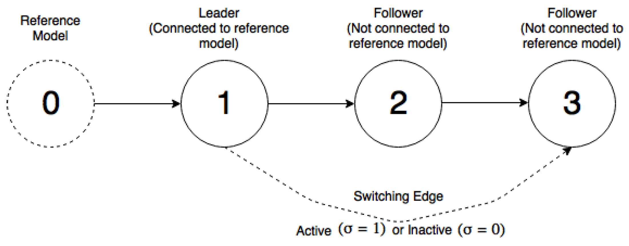
In practice, communication losses between agents may occur. Here, the communication loss is defined by a switching edge $\sigma$. If the switching edge is equal to zero, it means there is no communication between Agent 1 and Agent 3, and vice versa. The time-varying communication between Agent 1 and Agent 3 can change the network topology, which leads to different control structures in the form (42) or (27). The network topology where communication loss may occur between Agent 1 and Agent 3 is shown in Figure 3.

In order to prove the stability of the switched system, one can rely on the Lyapunov-based approach. In the case of Agent 3 with two parent neighbors, one can take the Lyapunov function as follows:

$$V_3({\tilde{\theta }}_3,{\tilde{x}}_{321})=\frac{{\tilde{x}}_{31}^{T}P{\tilde{x}}_{31}}{2}+\frac{{\tilde{x}}_{32}^{T}P{\tilde{x}}_{32}}{2}+\frac{{\tilde{\theta }}_3^T{\Gamma }_3^{-1}{\tilde{\theta }}_3}{2}\left|{\rho }_{321}^{*}\right|.$$

(49)

In the case of Agent 3 with one parent neighbor, one can take the Lyapunov function as follows:

$$V_3({\tilde{\theta }}_3,{\tilde{x}}_{32})=\frac{{\tilde{x}}_{32}^{T}P{\tilde{x}}_{32}}{2}+\frac{{\tilde{\theta }}_3^T{\Gamma }_3^{-1}{\tilde{\theta }}_3}{2}\left|{\rho }_{32}^{*}\right|$$

(50)

where ${\Gamma }_3={\Gamma }_3^T>0$ and $P=P^T>0$ such that (17) holds. It is clear that the Lyapunov function is not common to (49) and (50). This is because the Lyapunov function is influenced by the switching topology. Using the result in [19,20], we know that there is a dwell time for which stability can be derived. However, such a dwell time is unknown in the output-feedback case. Therefore, we conclude this work by proposing an adaptive switching scheme and by evaluating its effectiveness in simulations. 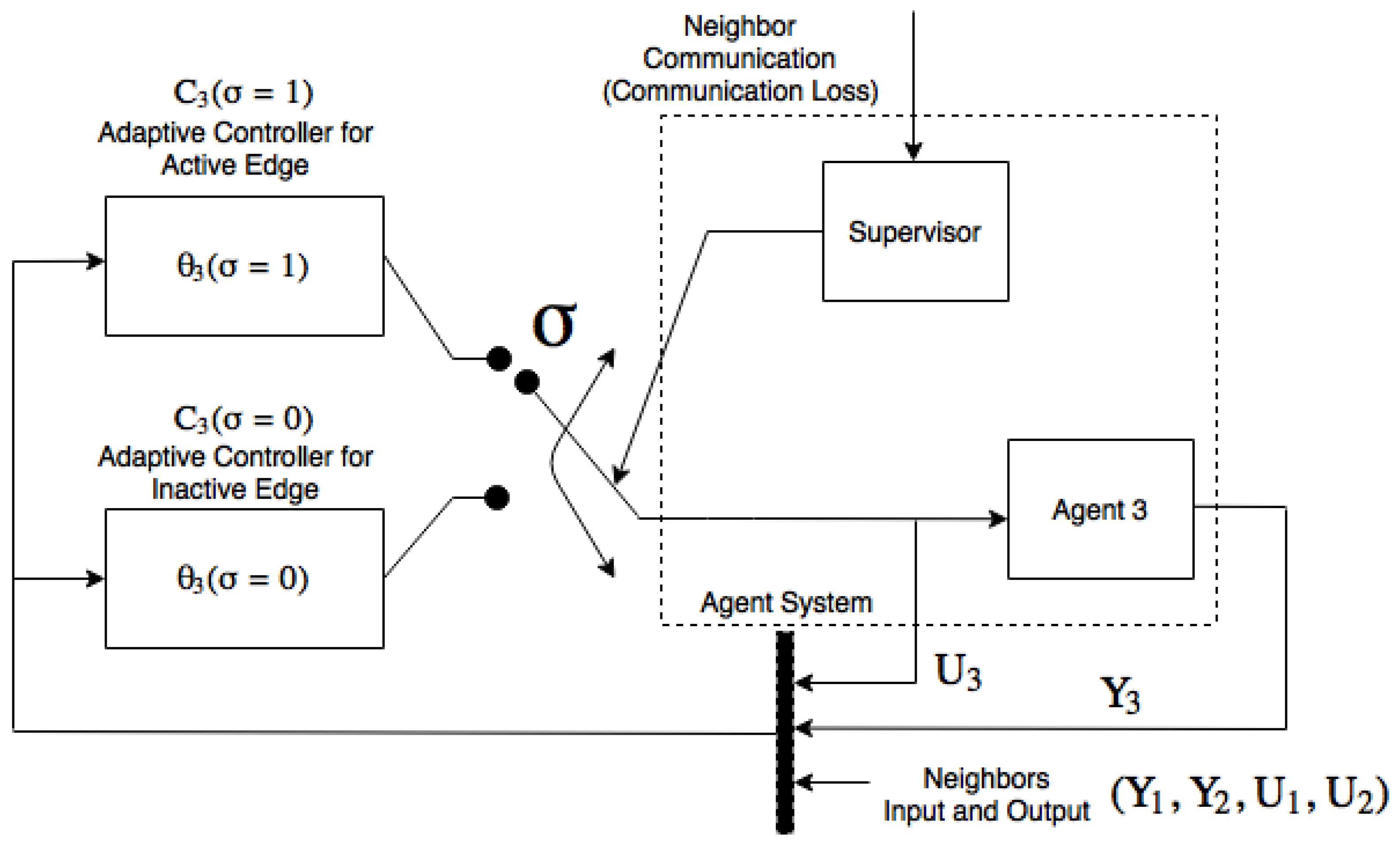The switching scheme resembles the multiple model adaptive control, e.g., as discussed in [22,23,24]. The switching adaptive controller that will be applied in this work is shown in Figure 4.

Here we have a free-running adaptive controller $C_3(\sigma =0)$ for an agent with one parent neighbor (Agent 2) and a reinitialized adaptive controller $C_3(\sigma =1)$ for an agent with two parent neighbors (Agent 1 and Agent 2). Then, let us define the adaptive controller parameter vectors ${\theta }_3(\sigma =1)$ and ${\theta }_3(\sigma =0)$. Note that, if the switching edge is inactive, the ${\theta }_3(\sigma =1)$ value should be held at its last value until the switching edge is active. Note also that ${\theta }_3(\sigma =0)$ is not affected by the switching edge because it only depends on Agent 2. Consider that, if the switching edge is inactive, the measurement of the input and the output of Agent 1 by Agent 3 are equal to zero.

4. Numerical Simulation

In line with [25,26], some simplified quadcopter dynamics are used as a numerical example. The simplified quadcopter attitude dynamics is given as follows:

$$\ddot{\psi }=I_y^{-1}{\tau }_{\psi }$$

(51)

where $\psi$, $I_y$, and ${\tau }_{\psi }$ are the yaw angle, the rotational moments of inertia on the y-axis, and the rotating torque on yaw angle, respectively. The yaw angle output will be utilized to synchronize the yaw angle for all the agents. The state–space representation of the quadcopter i with attitude dynamics:

$$\begin{array}{cc}\hfill {\dot{x}}_{\psi i}& =\left[\begin{array}{cc}0& 1\\ 0& 0\end{array}\right]x_{\psi i}+\left[\begin{array}{c}0\\ I_{yi}^{-1}\end{array}\right]{\tau }_{\psi }\hfill \\ \hfill y_{{\psi }_i}& =\left[\begin{array}{cc}1& 0\end{array}\right]x_{\psi i}\hfill \end{array}$$

(52)

where the state vector, $x_{\psi i}=[{\psi }_i,{\dot{\psi }}_i]$, comprises the yaw angle and the yaw rate, $i\in \{1,\dots ,N\}$, where N is the total number of the quadcopter. Note that (52) has relative degree 2 ($n^{*}=2$). Index 1 indicates the leader quadcopter, which is the only quadcopter that has direct access to the reference model. The reference model is indicated as fictitious Agent 0, which can communicate the reference signal to Agent 1. The reference model dynamics in state–space formulation is given as follows:

$$\begin{array}{cc}\hfill {\dot{x}}_{\psi 0}& =\left[\begin{array}{cc}0& 1\\ {\alpha }_1& {\alpha }_2\end{array}\right]x_{\psi 0}+\left[\begin{array}{c}0\\ I_{y0}^{-1}\end{array}\right]{\tau }_{\psi }\hfill \\ \hfill y_{{\psi }_0}& =\left[\begin{array}{cc}1& 0\end{array}\right]x_{\psi 0}\hfill \end{array}$$

(53)

where the model reference parameters are taken as: ${\alpha }_1=-0.5,{\alpha }_2=-1,I_{y0}=1$, and the initial condition of the reference model $[{\psi }_i,{\dot{\psi }}_i]=[1,-1]$. Each quadcopter has different and unknown rotational moments of inertia $I_y$, and the initial state is also unknown. Therefore, the network is composed of heterogeneous and unknown agents.

Table 1. Quadcopter parameters and initial conditions.

	${\mathit{I}}_{\mathit{yi}}$	$[{\mathit{\psi }}_{\mathit{i}},{\dot{\mathit{\psi }}}_{\mathit{i}}]$
Quadcopter 1	1	[1, 1]
Quadcopter 2	3	[−1, −1]
Quadcopter 3	2	[−1, 0]
Quadcopter 4	4	[0, 1]
Quadcopter 5	0.5	[1, 0]
Quadcopter 6	0.75	[−1, 1]

shows the parameters of each quadcopter that are used only to simulate the network.

In the next subsection, we will illustrate the synchronization of the MAS based on output-feedback MRAC with a fixed topology.

4.1. Multi-Agent Output-Feedback MRAC without Switching Topology

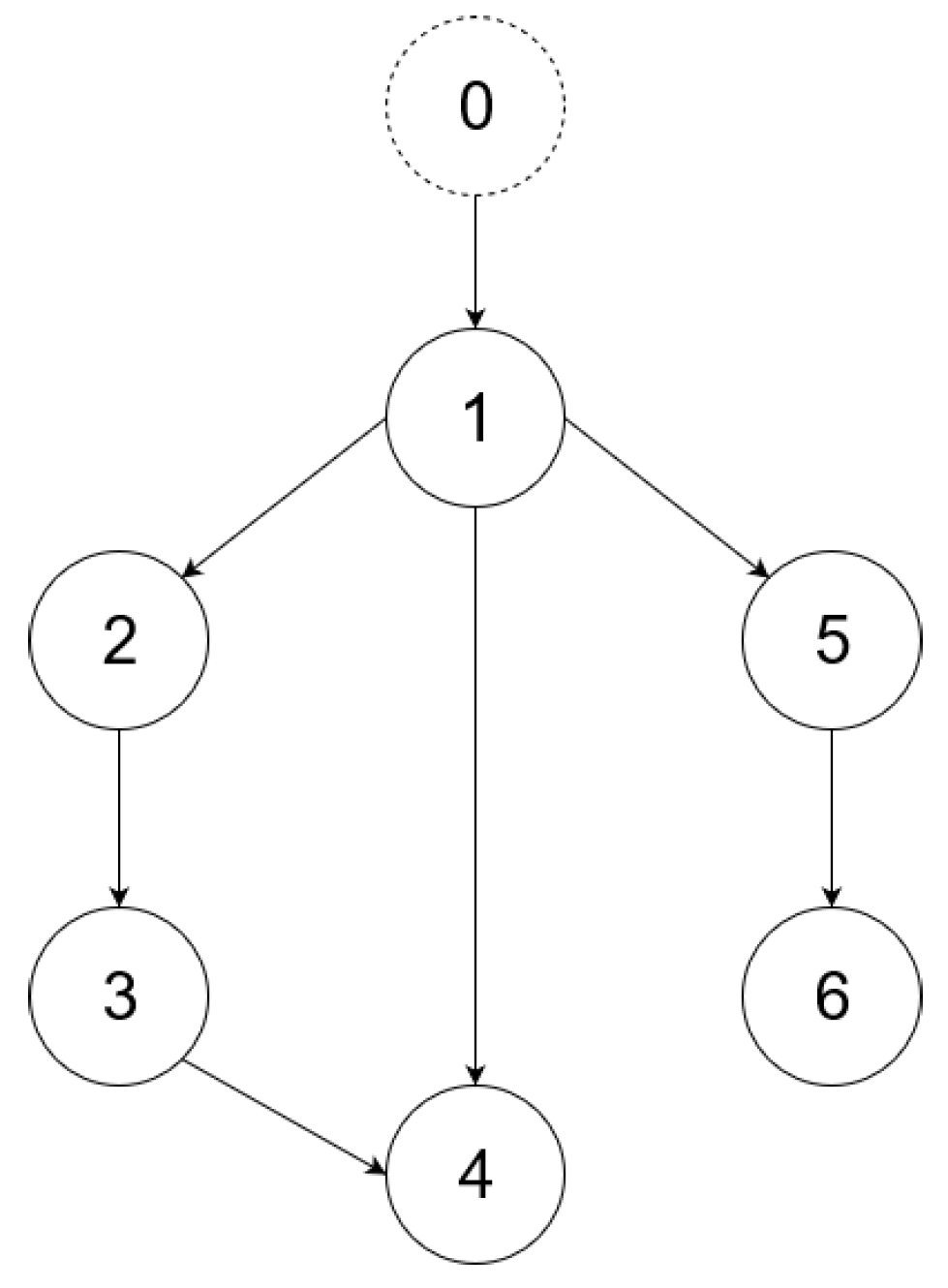
The simulations for multi-agent output-feedback MRAC with fixed topology are carried out on the directed graph shown in Figure 5. The design parameters are taken as $F=-0.7,\rho =0.3$, and all coupling vector gains are initialized to be 0. Let us define the adaptive gain ${\Gamma }_i$ for each agent i as follows:

$$\begin{array}{cc}\hfill {\Gamma }_1& =\mathrm{diag}\{{\Gamma }_l,{\Gamma }_f,{\Gamma }_g,{\Gamma }_c\}\hfill \\ \hfill {\Gamma }_2& ={\Gamma }_3={\Gamma }_5={\Gamma }_6=\mathrm{diag}\{{\Gamma }_l,{\Gamma }_f,{\Gamma }_g,{\Gamma }_c,{\Gamma }_l,{\Gamma }_f,{\Gamma }_g\}\hfill \\ \hfill {\Gamma }_4& =\mathrm{diag}\{{\Gamma }_l,{\Gamma }_f,{\Gamma }_g,{\Gamma }_c,{\Gamma }_l,{\Gamma }_f,{\Gamma }_g,{\Gamma }_c,{\Gamma }_l,{\Gamma }_f,{\Gamma }_g\}\hfill \end{array}$$

(54)

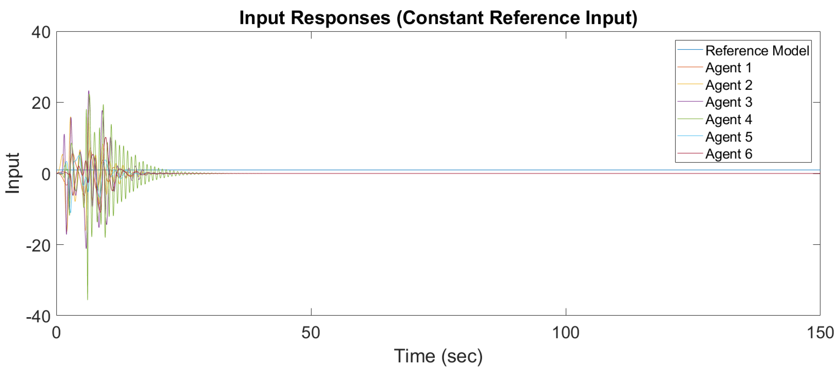
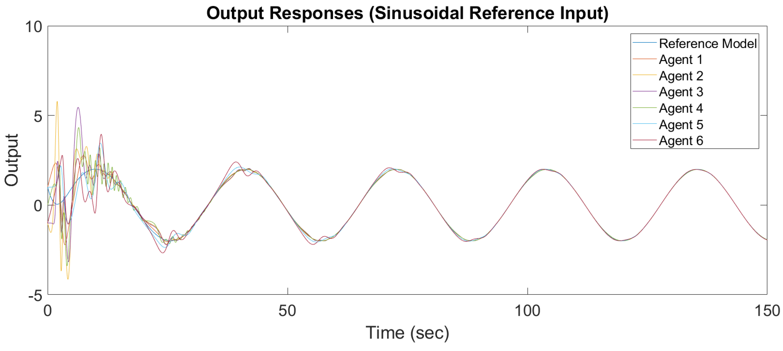
$\Gamma$ have been selected to give a smooth response and acceptable input action where ${\Gamma }_l=0.2$, ${\Gamma }_f=0.05$, ${\Gamma }_g=0.1$, and ${\Gamma }_c=0.025$. In our case, two reference inputs are considered:

• a constant reference input with an amplitude of 1;
• a sinusoidal reference input with a frequency of 0.2 rad/s and an amplitude of 1.

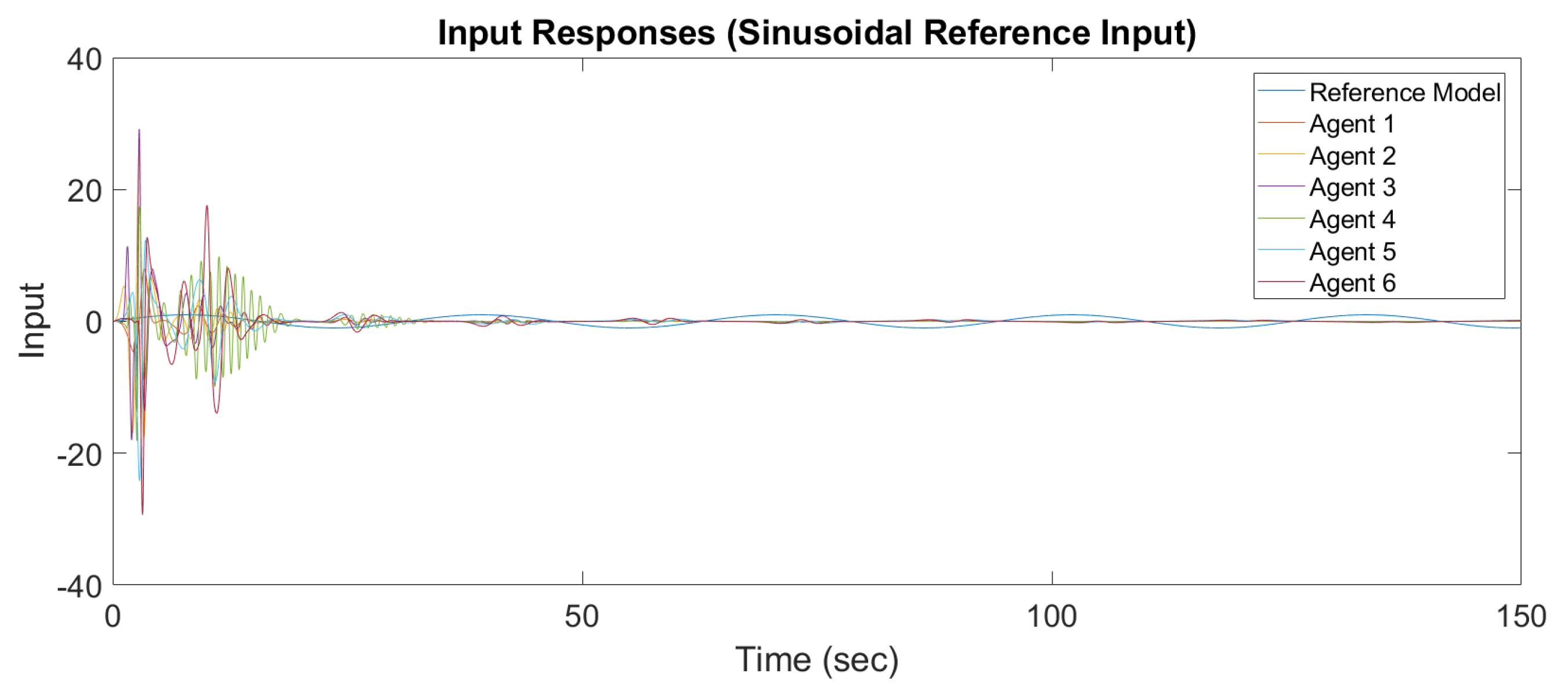
Figure 6 and Figure 7 show the output response and input response of synchronization with a constant reference input, and Figure 8 and Figure 9 show the output response and input response of synchronization with a sinusoidal reference input

It is observed that all outputs converge asymptotically to the output of the leader for constant and sinusodal leader inputs, respectively. The following subsection will illustrate the synchronization of the MAS with switching topology based on output-feedback MRAC.

4.2. Multi-Agent Output-Feedback MRAC with Switching Topology

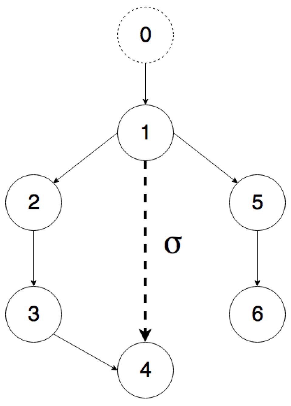
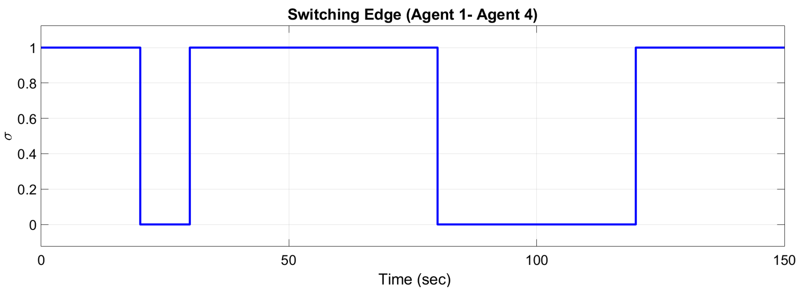
The simulations for multi-agent output-feedback MRAC with switching topology are carried out on the directed graph shown in Figure 10. The communication between Node 4 and Node 1 varies with time, e.g., due to communication losses. It must be noted that Agent 4 only has one parent neighbor if the edge is inactive and has two parents if the edge is active.

The activity or inactivity of the edge is defined by the switching edge of Figure 10 ($\sigma =1$, edge is active and $\sigma =0$, edge is inactive). The switching edge signal is shown in Figure 11. If the controller is not switching, Agent 4 continues to use the controller for two neighbors instead of only one. Note that the parameters of Agent 1 are equal to zero when there is no connection.

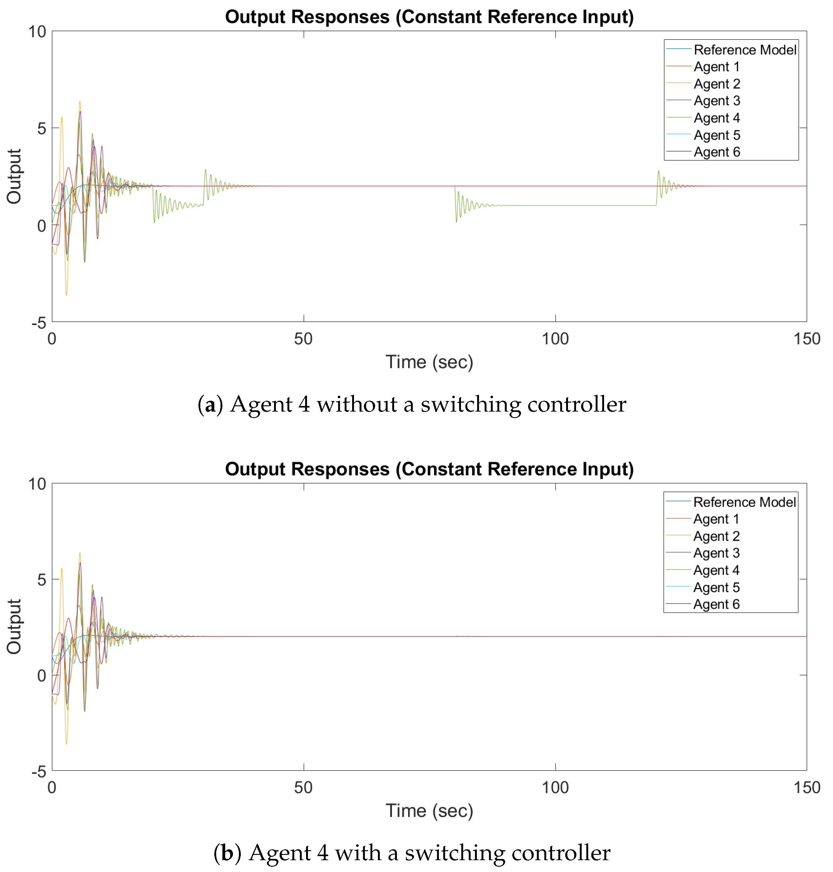
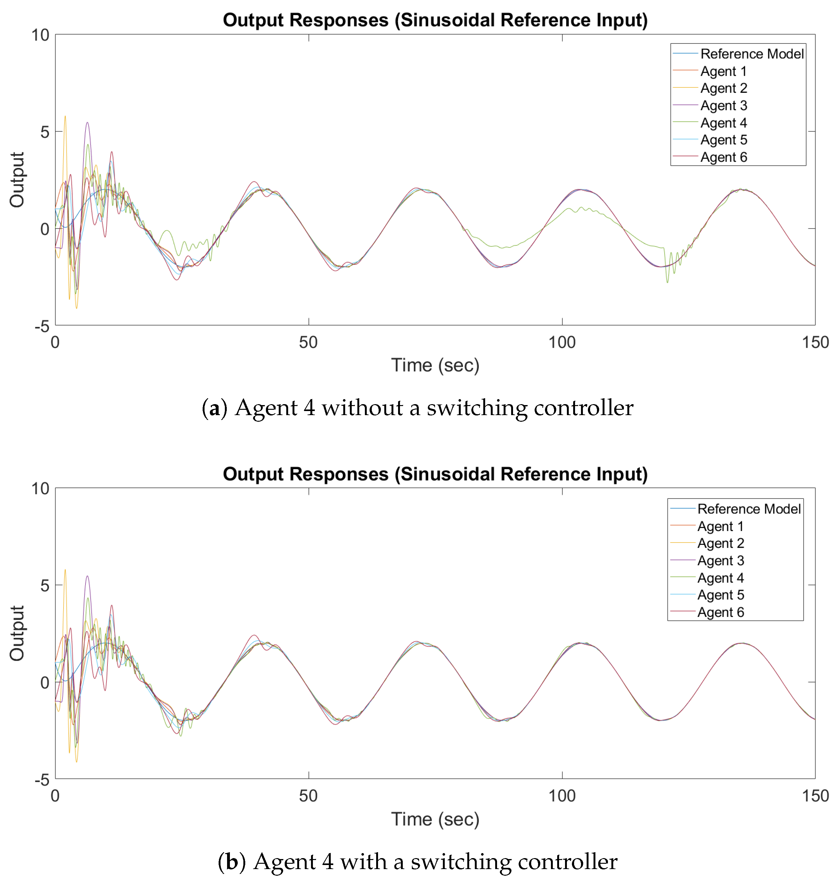
The design parameters and the reference inputs are the same as the design parameters and the reference inputs in the previous subsection. The output response of synchronization with a constant reference input and a sinusoidal reference input are shown in Figure 12 and Figure 13, respectively.

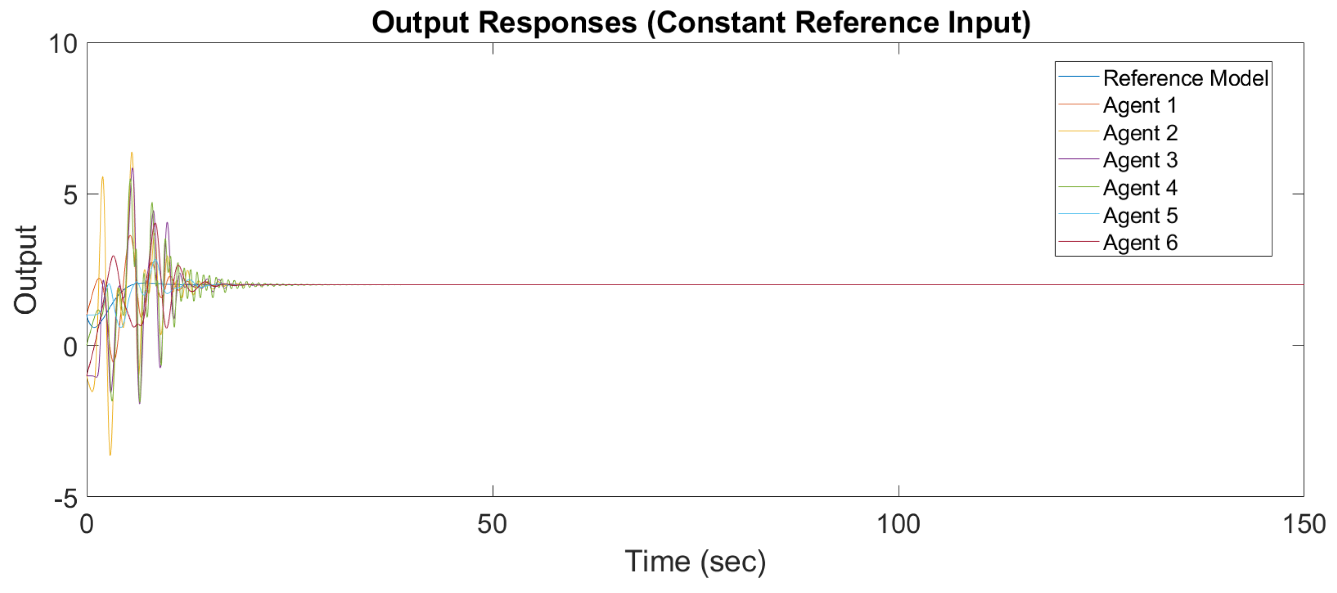
It can be observed in Figure 12a and Figure 13a that the output of Agent 4 does not converge to the output of the leader, while in Figure 12b and Figure 13b all the outputs converge asymptotically to the output of the leader. It can be concluded that, in the case of switching topologies, the switching adaptive controller must be implemented.

5. Conclusions

In this work, it was shown that the output synchronization of a heterogeneous MAS with unknown dynamics can be achieved through output-feedback MRAC. New adaptive laws were formulated for the controller parameter vector by using a matching condition assumption. In contrast with standard MRAC, where the adaptive gain is scalar-valued, in this work, the adaptive gain is a diagonal matrix. By using the proposed control law, the agents only require the output and the control input of its neighbors. This approach provides much convenience in the design and application of MAS synchronization because it does not require global information (e.g., the Laplacian matrix or algebraic connectivity). In order to have the synchronization error converge asymptotically to zero and to achieve bounded stability, a Lyapunov-based approach was derived analytically. In addition, a distributed switching controller was proposed to handle communication losses that deteriorate the synchronized response. Finally, numerical simulations were provided to validate the proposed method. It was shown that the convergence of the synchronized response can be achieved for a network with fixed or switching topologies.

Future work will include handling networks with possibly directed cycles; in the presence of cycles or loops, we expect a specific condition to ensure the stability of the proposed approach. The study of robustness in the presence of bounded disturbances could be an extension of the proposed output-feedback MRAC. Another exciting research direction could consist in exploring the possibility of handling system constraints (e.g., input constraints/actuator position saturation) for synchronization of MASs [27,28]. Another avenue worth investigating is the extension to state/output synchronization of nonlinear systems.