A Machine Learning Framework for the Prediction of Propeller Blade Natural Frequencies

Abstract

Characterization of propeller blade vibrations is essential to ensure aerodynamic performance, minimize noise emissions, and maintain structural integrity in aerospace and unmanned aerial vehicle applications. Conventional high-fidelity finite-element and fluid–structure simulations yield precise modal predictions but incur prohibitive computational costs, limiting rapid design exploration. This paper introduces a data-driven surrogate modeling framework based on a feedforward neural network to predict natural vibration frequencies of propeller blades with high accuracy and a dramatically reduced runtime. A dataset of 1364 airfoil geometries was parameterized, meshed, and analyzed in ANSYS 2024 R2 across a range of rotational speeds and boundary conditions to generate modal responses. A TensorFlow/Keras model was trained and optimized via randomized search cross-validation over network depth, neuron counts, learning rate, batch size, and optimizer selection. The resulting surrogate achieves $R^2>0.90$ and $NRMSE<0.08$ for the second and higher-order modes, while reducing prediction time by several orders of magnitude compared to full finite-element workflows. The proposed approach seamlessly integrates with CAD/CAE pipelines and supports rapid, iterative optimization and real-time decision support in propeller design.

1. Introduction

Propeller blades serve as fundamental elements in both manned and unmanned aerial platforms, where their dynamic behavior directly impacts aerodynamic performance, acoustic signature, and structural resilience. Accurate characterization of blade vibration modes is essential to prevent resonance, reduce noise emissions, and ensure long-term reliability under varying operational loads. Conventional design paradigms employ high-fidelity finite element analysis in conjunction with computational fluid dynamics to resolve complex fluid–structure interactions and compute natural frequencies. While these techniques yield precise modal predictions, they demand extensive computational resources and lengthy runtimes, thereby constraining the number of design iterations and inhibiting real-time decision making during early-stage development.

The emergence of machine learning algorithms provides a compelling avenue for constructing surrogate models that replicate numerical simulation outputs at a fraction of the computational cost. By learning the relationships among blade geometry, material properties, boundary conditions, and vibratory response, data-driven frameworks can execute thousands of design evaluations in near real time. Such accelerated analyses enable comprehensive exploration of design spaces, support uncertainty quantification, and facilitate integration into optimization loops and digital twin environments. Despite growing interest in surrogate modeling for turbomachinery components, the application to propeller vibration remains relatively unexplored, particularly in capturing higher-order modes and complex boundary effects.

This study introduces a systematic framework for predicting the natural vibration frequencies of propeller blades using a feedforward neural network. A database of 1364 distinct airfoil geometries was generated and subjected to modal analysis in ANSYS under a variety of rotational speeds and boundary constraints to produce a comprehensive training set. The airfoil database was obtained from the UIUC Airfoil Database [1], and thin and exotic airfoils were removed. A TensorFlow/Keras model was then trained and optimized through randomized search cross-validation across network depth, neuron counts, learning rate, batch size, and optimizer selection. The resulting surrogate model achieves a high coefficient of determination and low normalized root mean square error for the second and higher-order modes, while reducing prediction time by several orders of magnitude compared to full finite-element workflows.

The remainder of this paper is organized as follows. Section 2 provides a review of related work on machine learning in rotorcraft and propeller design. Section 3 provides the materials and methods, and describes the data generation pipeline, including geometry parametrization and simulation setup. Section 4 details results and discussion. Finally, Section 5 concludes with a summary of contributions and outlines future resarch directions aimed at further enhancing surrogate model fidelity and generalization.

2. Literature Review

The application of machine learning (ML) and computational methods has significantly advanced propeller and rotorcraft design, optimizing performance, reducing noise emissions, and improving structural stability. Across various studies, researchers have explored different methodologies to enhance efficiency, aerodynamics, and acoustic properties in aerospace, marine, and unmanned systems.

Recent advances in deep learning have reignited interest in data-driven simulation of physical systems [2]. Deep neural networks (DNNs) excel at learning intricate nonlinear mappings when supplied with abundant, high-fidelity data, enabling accurate outcome prediction purely from observed inputs [3]. Fundamentally, this data-driven approach relies entirely on neural networks inferring the system’s inherent dynamics from raw observations, without any explicit incorporation of the governing physical laws [4,5]. However, their performance degrades markedly under conditions of data sparsity or excessive noise, leading to poor generalization and unreliable extrapolation [6].

One branch of research addresses this limitation by constructing purely data-driven surrogate or reduced-order models using vast volumes of experimental or computational data [7,8]. While these surrogate models can achieve impressive accuracy, they often neglect fundamental physical constraints, behaving as opaque “black boxes” that may violate conservation laws and demand extensive data acquisition and careful experiment design, which can be computationally and logistically expensive [9].

A complementary paradigm embeds known physics directly into the training of DNNs, giving rise to physics-informed or physics-constrained neural networks [10,11,12]. By incorporating governing equations (e.g., partial differential equations) into the loss function, these networks can produce accurate solutions even with scarce or unlabeled data [13]. The imposed physical constraints act as a regularizer, mitigating overfitting, reducing dependence on large datasets, and enhancing predictive robustness by enforcing adherence to fundamental laws throughout learning [14].

Several studies apply machine learning techniques to optimize propeller design for improved aerodynamic efficiency, structural stability, and sustainability. Doijode et al. [15] utilized orthogonal parametric modeling and clustering algorithms to identify key design-variable correlations that enhance propeller performance while reducing greenhouse gas emissions. Their explainable ML models, validated using silhouette scores and Gaussian process regression (GPR), align well with experimental data, though limitations remain in capturing non-conformal geometry modifications and blade-hub interactions. Vardhan et al. [16] proposed the PropDesigner framework, integrating random forest regression (RF) with evolutionary algorithms to identify high-efficiency geometries. By achieving up to 90% efficiency compared to  50% in conventional designs, the study highlights the potential of hybrid ML-evolutionary approaches and suggests neural network integration and high-fidelity simulations for future refinement.

Structural analysis and material optimization further support performance improvements. Ahmad et al. [17] used finite element analysis (FEA) to evaluate quadcopter propellers made of carbon fiber-reinforced polymer (CFRP), identifying configurations with high resonance frequencies (183–1352 Hz) and minimal deformation. Similarly, Kilikevicius et al. [18] explored aeroelastic effects in flexible fiberglass propellers, demonstrating up to 2.2% speed gains through improved resonance alignment with operational ranges. Dahal et al. [19] focused on high-altitude UAV applications, optimizing fixed-pitch aluminum alloy propellers via blade element theory (BEM) and validating designs through computational fluid dynamics CFD and experiments. Structural integrity and modal safety are confirmed through stress and vibration analyses, despite observed discrepancies in thrust due to test-environment variations.

Acoustic prediction and noise mitigation are critical for both aerial and marine applications. Li and Lee [20] developed a framework using artificial neural networks (ANNs) and linear regression for broadband noise prediction in urban air mobility (UAM), with ANNs significantly outperforming traditional solvers in speed and frequency-domain accuracy. However, model opacity and simplified parameter interactions remain challenges. Legendre et al. [21] integrated CFD and computational aeroacoustics simulations with regression models such as gradient boosting regression (GBR) and random forest (RF) to enable real-time noise spectrum prediction for UAVs. Their system includes a graphical interface that assists in evaluating rotor speed effects on noise profiles, with results consistent with experimental benchmarks. In the marine domain, Xie et al. [22] developed a semi-analytical vibro-acoustic model of submarine propeller-shaft-hull systems, achieving high accuracy and computational efficiency by replacing traditional FEM/BEM techniques. The study reveals that breathing modes dominate acoustic radiation and that bearing stiffness significantly impacts vibro-acoustic behavior.

Advancements in surrogate modeling and optimization have also improved marine propeller design. Uslu et al. [23] introduced a frequency reduction ratio for modal analysis in water, enhancing the accuracy of fluid-structure interaction models under submerged conditions. Gypa et al. [24] presented an interactive optimization system combining genetic algorithms and support vector machines (SVMs), incorporating human input to balance cavitation risks and performance. The SVM surrogate model effectively reduces manual evaluation needs while improving design iteration efficiency.

Recent research has increasingly incorporated physics-informed and federated learning paradigms. Soibam et al. [25] proposed an ensemble physics-informed neural network (PINN) framework for inverse flow and thermal field reconstruction. By embedding the Navier–Stokes and energy equations in the loss function and enforcing optimal sensor placement, they achieve sub-10% relative errors with high uncertainty quantification and robust performance from minimal sensor data. Similarly, Vermelin et al. [26] applied federated learning (FedAvg, FedPer) with long short-term memory (LSTM) and ConvGRU architectures for remaining useful life (RUL) prediction across non-IID datasets. Their privacy-preserving approach matches or exceeds local baselines on SiC-MOSFET and turbofan benchmarks, with minimal degradation under realistic network constraints. The study suggests applicability to distributed propeller-blade data without violating data governance.

Emerging diagnostic and decision-support systems further expand ML’s role. Soibam et al. [27] achieved high-precision (96% AP at IoU = 0.5) bubble segmentation in two-phase flows using a CNN-based instance segmentation model (YOLOv7 + YOLACT++), leveraging transfer learning and demonstrating robustness to noise and dynamic phenomena. Their pipeline extracts localized geometric statistics with minimal error, offering parallels to propeller-blade vibration modeling, where such descriptors could enhance low-cost ML predictions. Mählkvist et al. [28] introduced a cost-sensitive classification framework for industrial batch processes, using confidence thresholds and relative cost matrices to balance accuracy and deployment cost. Their approach reduces relative operational risk by up to 74% compared to baseline and illustrates potential trade-offs between prediction certainty and simulation effort in propeller design workflows.

Netzell et al. [29] offered a comprehensive methodology for input derivation and validation in time-series forecasting. By applying rolling-origin evaluation, MSTL decomposition, and lag-matched training, they reduce RMSEs significantly for electric-load prediction. Their protocol, emphasizing rigorous feature selection and retraining cadence, serves as a model for structuring inputs in propeller frequency prediction, balancing model accuracy and computational efficiency.

The present work proposes an automated end-to-end CAD/CAE to machine learning pipeline that makes high-fidelity modal prediction for propeller blades practical within design time frames. It explicitly incorporates rotational effects in the modal simulations and assembles a large and diverse multi-profile simulation corpus to train data-driven surrogates. Through a careful and systematic benchmark across different families of learning algorithms, the work shows that trained surrogates can reach high predictive accuracy while substantially reducing the time needed to obtain modal estimates compared with full finite element analysis, and that different model families display complementary strengths depending on the frequency band. The work is innovative in integrating an automated CAD and CAE workflow, explicit treatment of rotational modal effects, a broad multi-profile simulation corpus, and a comprehensive comparison of machine learning methods to produce rapid and accurate modal surrogates for propeller blades, thereby closing the gap between high-fidelity analysis and time-limited design practice.

In summary, advancements in ML, computational modeling, and optimization techniques have significantly improved propeller and rotorcraft design across various domains. These studies collectively underscore the importance of integrating data-driven approaches with traditional engineering methodologies to achieve sustainable, high-performance solutions, paving the way for future innovations in aerospace, marine, and UAV applications.

The novelty of this study lies in the integration of an automated CAD–CAE pipeline with machine learning to predict the natural frequencies of rotating propeller blades across a wide design space. Unlike existing studies that rely on limited geometries or simplified physics, this work combines a large and diverse airfoil database with fully automated ANSYS modal analyses that include rotational effects. In addition, a systematic comparison of multiple machine learning models is conducted using a consistent training and evaluation protocol, demonstrating the suitability of machine learning models as accurate for both low- and high-order modal predictions.

3. Materials and Methods

3.1. Modal Analysis

In this study, we process a comprehensive database of airfoil profiles to simulate the natural frequencies of propeller blades. The database consists of 1364 distinct airfoil shapes, initially stored in a CSV format. These airfoils were processed in MATLAB 2024b to simplify their geometrical representation by reducing the number of coordinate points. This simplification step was necessary to streamline subsequent stages such as geometry generation and mesh creation, as fewer coordinates facilitate faster processing without sacrificing the essential geometric characteristics of the airfoils.

3.1.1. Geometry

The airfoil profiles were imported and used to generate propeller geometries. At each radial station along the blade span, the corresponding airfoil was positioned accordingly. Each propeller geometry was composed of five distinct airfoils, each assigned a specific chord length. The twist angle $\beta$ for each airfoil was calculated using the following equation:

$$\beta ={tan}^{-1}\left({\displaystyle \frac{V}{\omega r}}\right)$$

(1)

where V is the axial velocity, $\omega$ is the rotational velocity, and r is the radial position.

This definition was introduced at the geometry generation stage and consistently applied to all configurations, implicitly assuming a zero geometric angle of attack along the blade span. The assumption was adopted to ensure a simple, fully automated, and numerically robust blade-generation process, avoiding the need for airfoil-dependent aerodynamic data or iterative pitch optimization. While this does not represent aerodynamically optimal operation, its influence on the predicted natural frequencies is expected to be small.

The parameters were generated based on a uniform distribution within the ranges specified in

Table 1. Propeller simulation parameter ranges.

Parameter	Minimum Value	Maximum Value	Unit
Diameter	0.40	5.60	m
Rotational Velocity	50	1350	rad/s
Velocity	8	112	m/s
Chord #1	0.06	0.24	m
Chord #2	0.11	0.29	m
Chord #3	0.16	0.34	m
Chord #4	0.16	0.34	m
Chord #5	0.06	0.24	m
Hub/Diameter	0.05	0.15	-
Airfoil ID #1	1	1364	-
Airfoil ID #2	1	1364	-
Airfoil ID #3	1	1364	-
Airfoil ID #4	1	1364	-
Airfoil ID #5	1	1364	-

. The resulting feature set comprises 14 core feature categories, including two operating parameters (rotational velocity and axial inflow velocity) and seven geometric parameters corresponding to the chord lengths at five radial stations along the blade, propeller diameter, and hub-to-diameter ratio. In addition, the airfoil shape at each radial station is defined through discrete airfoil identifiers, which encode the local aerodynamic profile used in the blade design.

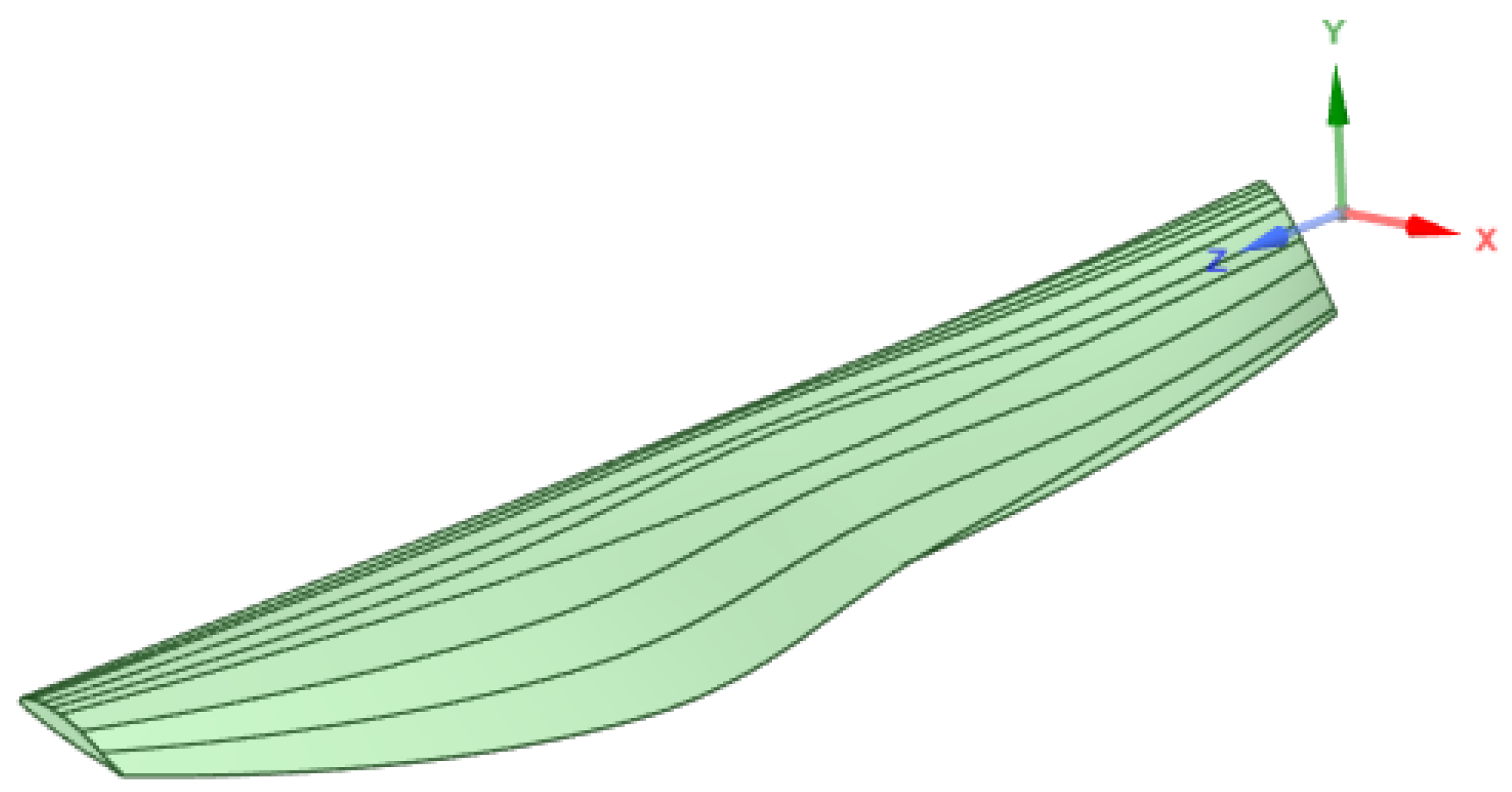
Each normalized airfoil at its corresponding radial location was scaled according to its designated chord length and rotated based on its pitch angle. Once all airfoils were properly configured, a loft operation was performed to generate the tridimensional propeller geometry. Figure 1 and Figure 2 illustrate this process, which was carried out in ANSYS through Python 3.12 scripts.

3.1.2. Mesh

The mesh was generated using the adaptive sizing option, which smoothed the geometry and model features. The resolution was set to 6, representing a moderately fine mesh level. Small geometric details that do not significantly affect the simulation were ignored, contributing to more robust mesh generation. Tetrahedral elements were used to discretize the geometry, as they are well-suited for complex 3D shapes and ensure better conformity to curved surfaces and intricate features.

The entire meshing process was automated within the ANSYS Workbench environment to ensure full integration with the parametric geometry generation workflow. The mesh settings were intentionally chosen to be general-purpose and adaptable, aiming to guarantee robust meshing across the entire range of geometries produced. Since the generated propellers vary significantly in size due to the design space exploration, using fixed meshing parameters would likely result in poor mesh quality or even failure in mesh generation for certain cases.

A mesh-convergence study was performed using ANSYS mesh resolutions from 2 to 7 (resolution 7 is the largest available in ANSYS) to evaluate the trade-off between computational cost and numerical accuracy. For each resolution, we recorded the meshing time and the first ten natural frequencies for a representative geometry; relative differences with respect to the finest resolution (7) were computed to quantify the numerical changes. Results are presented in

Table 2. Mesh resolution convergence study. Top: mesh size and meshing time for each tested resolution. Middle: first ten natural frequencies (Hz) for a representative case at resolutions 2–7. Bottom: relative differences with respect to resolution 7 (in %).

	Resolution
	2	3	4	5	6	7
Nodes	6053	6162	7174	9220	11,902	21,739
Elements	2875	2903	3426	4442	5970	11,322
Time [s]	7.12	7.78	7.92	8.42	9.37	11.35
Natural frequencies (Hz, representative case)
1	2.7329	2.7107	2.7089	2.7049	2.7020	2.6980
2	23.355	23.142	23.115	23.073	23.055	23.017
3	77.184	76.922	76.913	76.866	76.843	76.824
4	188.59	188.40	188.26	188.05	188.00	187.91
5	258.51	258.01	257.87	257.66	257.52	257.37
6	309.54	308.60	308.24	307.36	307.08	306.59
7	446.61	445.23	444.77	443.80	443.47	442.95
8	504.45	503.97	502.95	501.30	500.43	499.44
9	622.73	623.03	621.44	620.00	619.22	618.14
10	721.00	720.71	715.81	710.68	708.24	703.98
Relative difference vs. resolution 7 (%)
1	1.29%	0.47%	0.40%	0.26%	0.15%	–
2	1.47%	0.54%	0.43%	0.24%	0.17%	–
3	0.47%	0.13%	0.12%	0.05%	0.02%	–
4	0.36%	0.26%	0.19%	0.07%	0.05%	–
5	0.44%	0.25%	0.19%	0.11%	0.06%	–
6	0.96%	0.66%	0.54%	0.25%	0.16%	–
7	0.83%	0.51%	0.41%	0.19%	0.12%	–
8	1.00%	0.91%	0.70%	0.37%	0.20%	–
9	0.74%	0.79%	0.53%	0.30%	0.17%	–
10	2.42%	2.38%	1.68%	0.95%	0.61%	–
Mean	1.00%	0.69%	0.52%	0.28%	0.17%	–

. The study shows that the incremental gain in modal accuracy becomes marginal for the finest resolutions, while the CPU time increases noticeably.

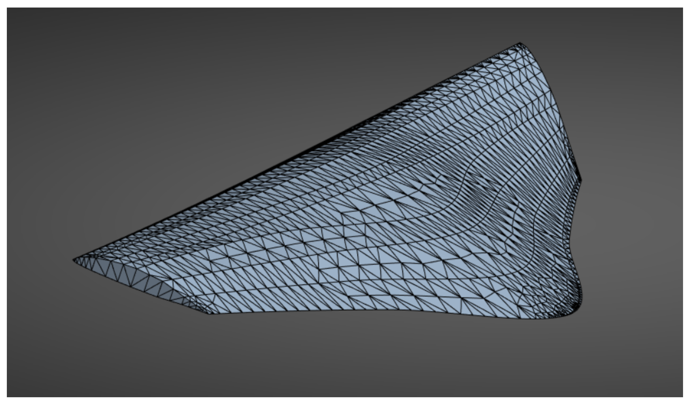
By employing adaptive sizing, tetrahedral elements, and dynamic resolution settings, the meshing process was made flexible enough to accommodate significant variations in propeller geometry, while maintaining consistency and reliability across all simulations. This approach resulted in meshes with approximately 12,000 nodes, striking a balance between computational efficiency and simulation accuracy. The employed mesh size is also larger than that used in Alarcón et al. [30], who employed a mesh containing 7553 nodes to validate a propeller simulation in ANSYS Mechanical Modal against experimental results. A dedicated mesh-convergence study (Table 2) showed that increasing the ANSYS resolution above 6 produced only marginal improvements in the predicted natural frequencies (mean relative change of about 0.17% between resolution 6 and the finest available resolution 7), while the meshing time increased from approximately 9.37 s (resolution 6) to 11.35 s (resolution 7), an increase of roughly 21% in computational cost. For this reason, resolution 6 was selected as the working mesh setting, since it provides an excellent compromise between numerical fidelity and computational efficiency. Figure 3 presents an example of a generated mesh, highlighting the adaptability and quality of the automated meshing strategy. The highlighted geometry generation parameters are shown in

Table 3. Propeller simulation input values from script parameters.

Parameter	Value	Unit
Airfoil ID #1	1	–
Airfoil ID #2	2	–
Airfoil ID #3	3	–
Airfoil ID #4	4	–
Airfoil ID #5	5	–
Alpha #1	53.1300	deg
Alpha #2	22.3062	deg
Alpha #3	13.6269	deg
Alpha #4	9.7618	deg
Alpha #5	7.5946	deg
Chord #1	0.10	m
Chord #2	0.15	m
Chord #3	0.22	m
Chord #4	0.16	m
Chord #5	0.10	m
Hub	0.10	m
Diameter	3.00	m

.

3.1.3. Simulation

The simulations considered the rotational effects of the propeller on its natural frequencies. In the modal analysis of rotating propellers, these rotational effects introduce gyroscopic forces, which influence the system’s damping characteristics. To model these effects accurately, we adopted an approach that accounts for the Coriolis effect in a stationary reference frame during modal analysis.

The Coriolis effect, which acts perpendicular to both the motion of the object and the axis of rotation, introduces gyroscopic coupling into the equations of motion. Although this force does not dissipate energy, it significantly affects the system’s motion and alters the modal characteristics of the structure.

In ANSYS Mechanical APDL [31], the damped modal analysis considers not only the mass matrix $\left[M\right]$, stiffness matrix $\left[K\right]$, and damping matrix $\left[C\right]$, but also includes the gyroscopic (Coriolis) matrix $\left[G\right]$ when analyzing rotating systems. The equation of motion becomes

$$\left[M\right]\ddot{u}+\left(\left[C\right]+\left[G\right]\right)\dot{u}+\left[K\right]u=0$$

(2)

where

• $\left[M\right]$ is the mass matrix
• $\left[C\right]$ is the structural damping matrix
• $\left[G\right]$ is the gyroscopic matrix introduced by the Coriolis effect
• $\left[K\right]$ is the stiffness matrix
• u is the displacement vector

A total of 3000 geometries and meshes of blades were generated from the process mentioned. A Python script was also created in the ANSYS Mechanical Modal to ensure the proper functioning of the simulations by setting up the face corresponding to the innermost airfoil as the fixed boundary condition at the first airfoil surface, where the blade connects to the hub, and assigning the material to the body. This simulation setup was tested in the work of Alarcón et al. [30], in which the numerical model was validated using ANSYS Mechanical Modal Analysis and experimentally obtained results. Structural steel (Young’s modulus of 200 GPa, density of 7850 kg/m³, and Poisson’s ratio of 0.3) was selected as the material for the propeller blade. This choice ensures that the blade’s mechanical behavior is accurately simulated under the conditions of the analysis.

The first ten natural vibration frequencies were extracted for each model. Out of the 3000 propeller configurations simulated, 1985 models successfully converged, yielding reliable results for further analysis. For each of these converged models, the airfoil IDs were replaced with their corresponding coordinate data, generating a fully representative dataset for subsequent investigation.

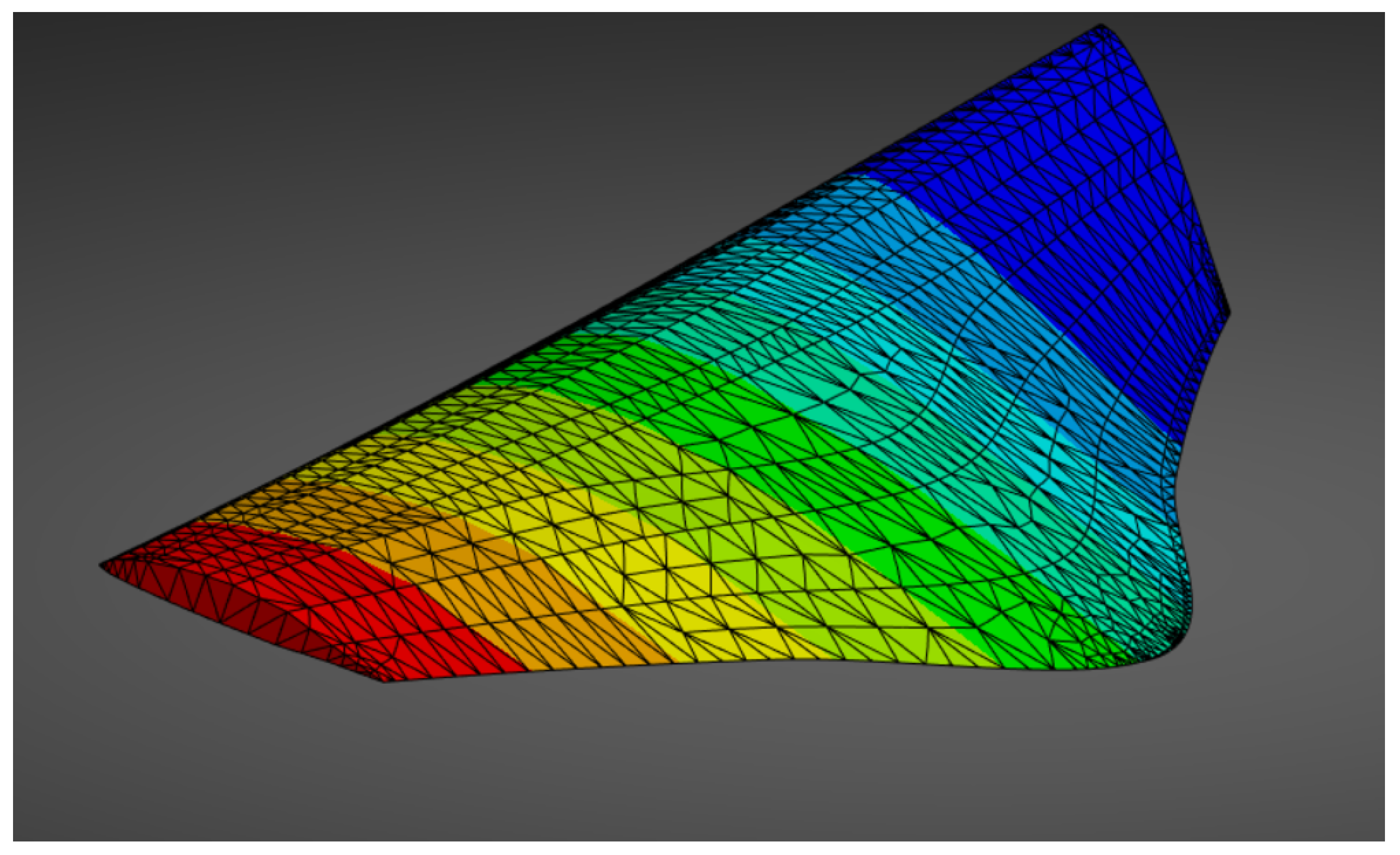
Figure 4 shows the modal shape of the first vibration mode for the same propeller geometry analyzed previously. The corresponding damped natural frequencies for the first ten modes are listed in

Table 4. Natural frequencies of the propeller.

Mode	Frequency [Hz]
1	2.70
2	23.06
3	76.84
4	188.00
5	257.52
6	307.08
7	443.47
8	500.43
9	619.22
10	708.24

.

3.2. Model Training

This chapter describes a streamlined training protocol applied uniformly to four machine learning models: random forest (RF), gradient boosting regressor (GBR), Gaussian process regressor (GPR), and a feedforward neural network (NN). The available dataset comprises records of 1985 individuals, and each model was trained and evaluated using progressively larger subsets of 500, 1000, 1500, and the full 1985 samples to investigate performance scaling. These experiments provide a comprehensive analysis of how model behavior varies with training set size. In all trainings, each subset was divided into training, validation, and test sets (80%/10%/10%).

The number of hyperparameter optimization iterations was defined empirically. After testing different iteration counts and analyzing the convergence behavior and performance gains for each algorithm, suitable values were identified that offered a good compromise between computational cost and model performance. Based on this empirical evaluation, 60 iterations were adopted for RF and GBR, 300 iterations for GPR, and 100 iterations for the NN.

3.2.1. Random Forest

The random forest model was implemented in Python using scikit-learn. Hyperparameter optimization was conducted with RandomizedSearchCV over the search space detailed in

Table 5. Hyperparameter search space for the random forest model.

Hyperparameter	Values
n_estimators	{50, 100, 150,…, 1000} (step 50)
max_depth	{None, 10, 20, 30, 40, 50, 60, 70, 80, 90, 100}
min_samples_split	{2, 5, 10, 20, 50}
min_samples_leaf	{1, 2, 4, 8, 16}
bootstrap	{True, False}

, employing 60 iterations and five-fold cross-validation for each training subset. The optimal estimator was then retrained on the corresponding training data and evaluated on the test set using the coefficient of determination ($R^2$) and normalized root mean squared error (NRMSE).

3.2.2. Gradient Boosting Regressor

The gradient boosting regressor model was implemented in Python using scikit-learn. Hyperparameter optimization is also performed using RandomizedSearchCV over the search space defined in

Table 6. Hyperparameter search space for the gradient boosting model.

Hyperparameter	Values
n_estimators	{50, 100, 150,…, 1000} (step 50)
learning_rate	{0.01, 0.05, 0.1, 0.2, 0.3, 0.5}
max_depth	{3, 5, 10, 20, 30, 40, 50}
min_samples_split	{2, 5, 10, 20, 50}
min_samples_leaf	{1, 2, 4, 8, 16}

, using 60 iterations and five-fold cross-validation.

3.2.3. Gaussian Process Regression

The GPR model was also implemented using scikit-learn. Hyperparameter optimization was conducted via random sampling over 300 trials, where each trial tested a different kernel configuration. The search space included combinations of RBF, Matern, and White kernels, with kernel hyperparameters (length scale, constant value, noise level, and regularization parameter $\alpha$) drawn from log-uniform distributions, which are presented in

Table 7. Hyperparameter search space for the GPR model.

Hyperparameter	Values/Range
length_scale	${10}^{[-1,2]}$ (log-uniform)
constant_value	${10}^{[-1,2]}$ (log-uniform)
noise_level	${10}^{[-4,0]}$ (log-uniform)
alpha	${10}^{[-8,-3]}$ (log-uniform)
kernel_choice	{RBF + White, Matern + White, RBF × Matern + White}

.

3.2.4. Neural Network Regression

A feedforward neural network model was implemented using TensorFlow and wrapped with scikeras for compatibility with scikit-learn tools. The neural network architecture consists of an input layer, a variable number of hidden layers with configurable neuron counts and activation functions, and a linear output layer with 10 neurons (one for each target variable). The model was compiled using mean squared error as the loss function and supports different optimizers such as SGD, RMSprop, Adam, and AdamW. Hyperparameter optimization was performed using RandomizedSearchCV across 100 trials, employing 5-fold cross-validation on the training set. The hyperparameter space included the number of hidden layers, the number of neurons, the learning rate, the batch size, and the optimizer type. Early stopping with a patience of 25 epochs was used to avoid overfitting during training. The hyperparameter search space for the neural network model is presented in

Table 8. Hyperparameter search space for the neural network model.

Hyperparameter	Values/Range
n_hidden	{2, 4, 6, 8, 10}
n_neurons	$[100,1000]$ (uniform integer)
learning_rate	${10}^{[-4,-0.7]}$ (log-uniform)
batch_size	{4, 8, 16}
optimizer	{SGD, RMSprop, AdamW, Adam}

.

4. Results and Discussion

In this section, we present a comprehensive evaluation of the four regression algorithms: Gaussian process regression (GPR), gradient boosting (GB), neural network (NN), and random forest (RF) across ten vibrational modes. The goal is to quantify each model’s ability to predict the modal frequencies from the provided feature set as the size of the training dataset varies. Two complementary performance metrics are employed—the coefficient of determination ($R^2$), which measures the model’s ability to explain the variance in the target, and the normalized root-mean-square error (NRMSE), which captures the prediction error relative to the observed range.

For each mode, we incrementally increase the number of training samples from 500 up to 2000 and record both $R^2$ and NRMSE. This allows us to analyze learning curves that reveal (i) the data efficiency of each algorithm, (ii) its convergence behavior, and (iii) its robustness across low, mid, and high-frequency regimes.

The machine used for the simulations and model training was an Intel Core i7 11800H (2.30 GHz) with 32 GB of RAM. Parallel processing was employed when possible. The CAE simulations to obtain natural frequency data took approximately 360 h. Each model training run required roughly 0.5 to 3 h, depending on the model and hyperparameter settings. While a single CAE simulation took around 10 min, the data-driven models took around 0.05–0.5 s to predict the natural frequencies,

4.1. Coefficient of Determination (R²)

This section presents the analysis of the coefficient of determination ($R^2$) for the evaluated models across different vibrational frequencies. The $R^2$ metric measures the proportion of variance in the target variable that is predictable from the input features, providing an overall indication of the model’s accuracy. The following figures illustrate how $R^2$ evolves as the size of the training dataset increases, offering insights into the learning behavior and performance scalability of each model.

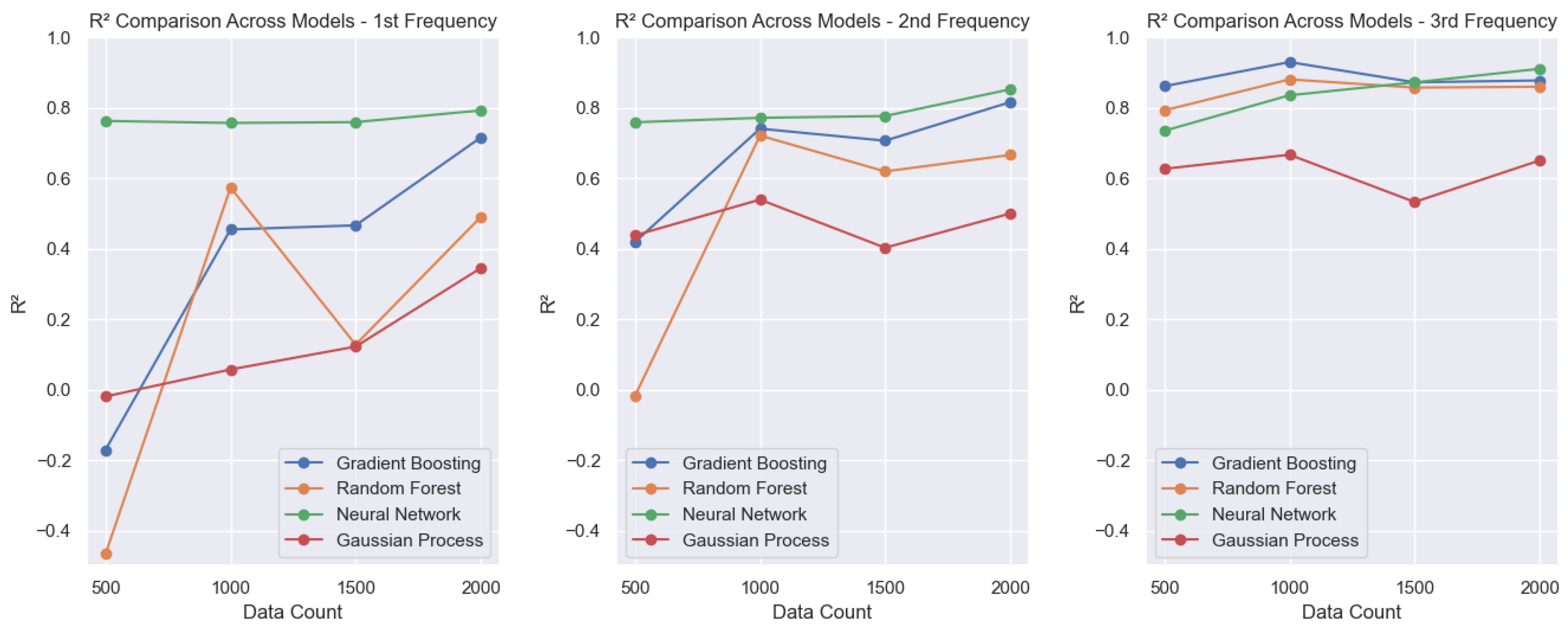
For the first three vibrational modes (Figure 5), all four algorithms exhibit a clear improvement in the coefficient of determination ($R^2$) as the training set size increases. The neural network (NN) model already achieves $R^2$ values close to 0.8 even with the smallest training set, showing steady improvements as more data becomes available. In contrast, for the first vibrational frequency, the GPR, gradient boosting (GB), and random forest (RF) models present poor performance, with $R^2$ values reaching negative levels when trained with only 500 samples. As the dataset grows, GB shows a notable improvement, reaching an $R^2$ of approximately 0.7, while RF and GPR remain with unsatisfactory $R^2$ scores. For the second frequency, GB continues to outperform, achieving an $R^2$ of around 0.8, whereas RF and GPR still underperform. In the case of the third frequency, only the GPR model maintains a comparatively lower performance, with $R^2$ values of around 0.6, while the other models perform considerably better.

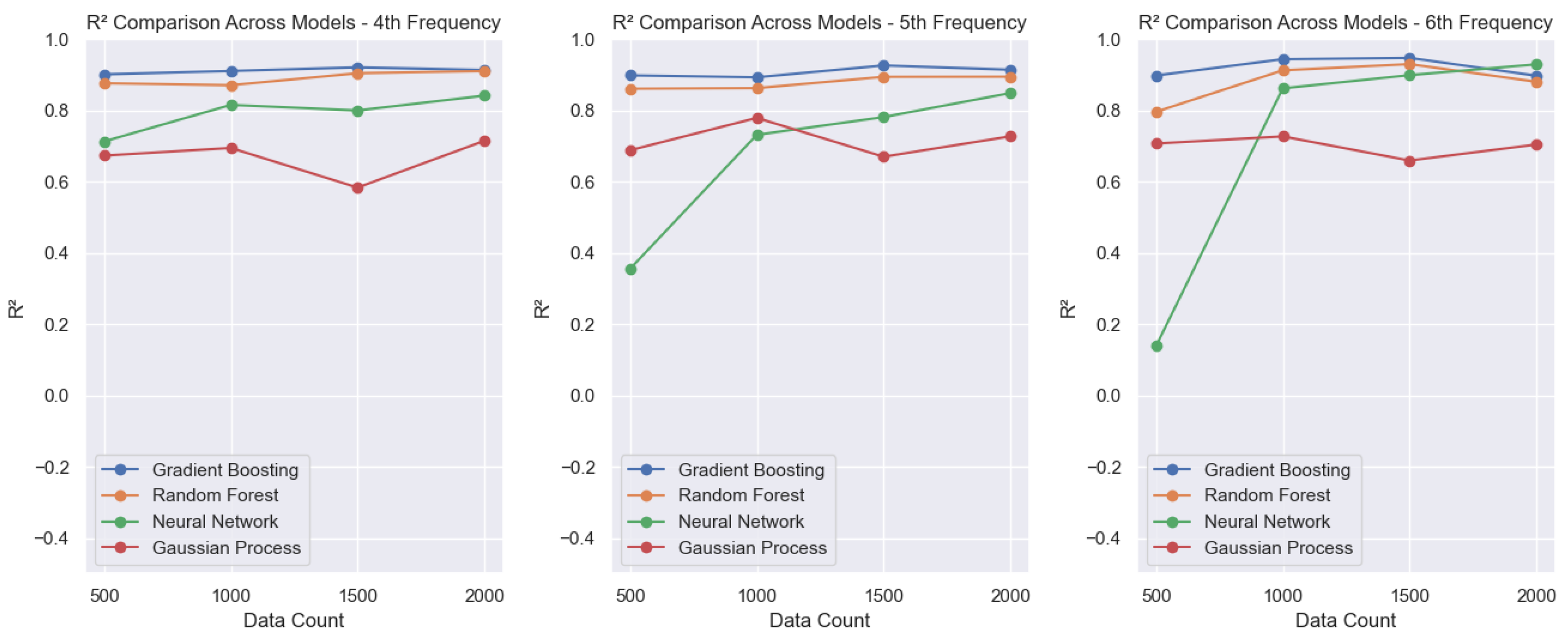
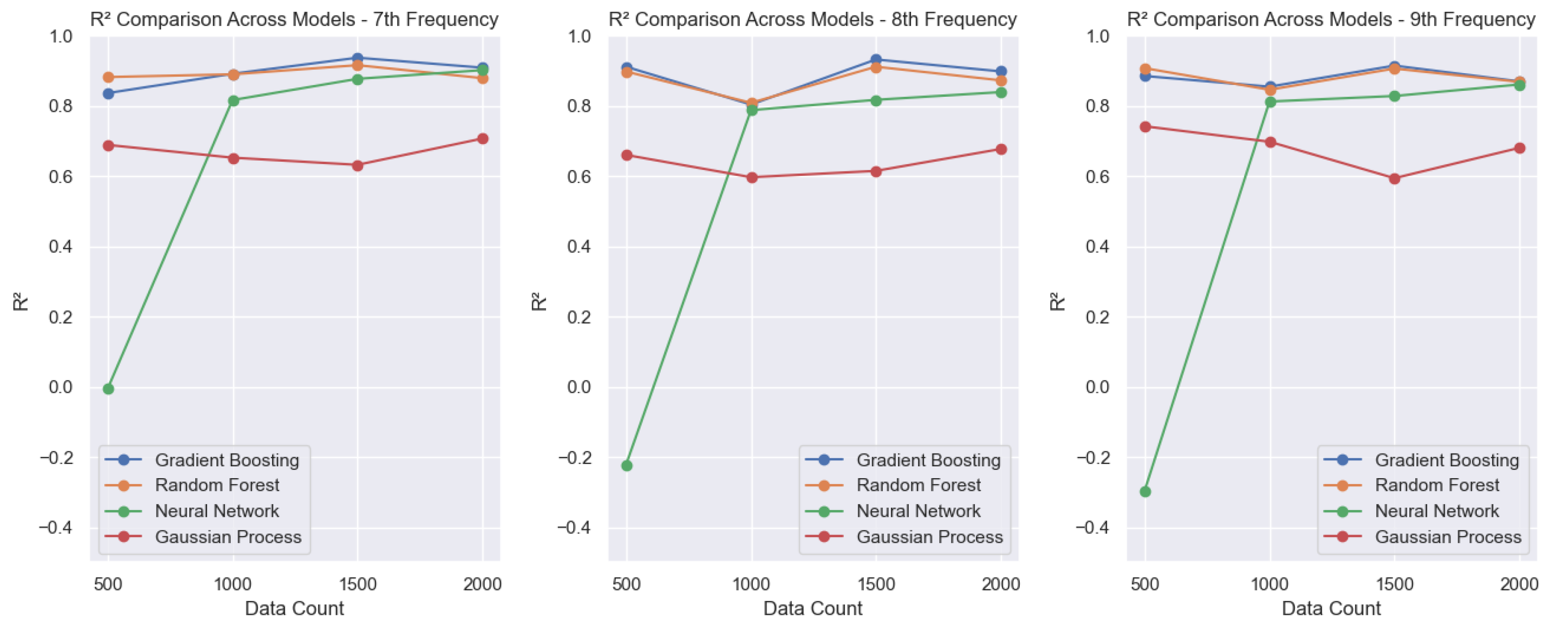
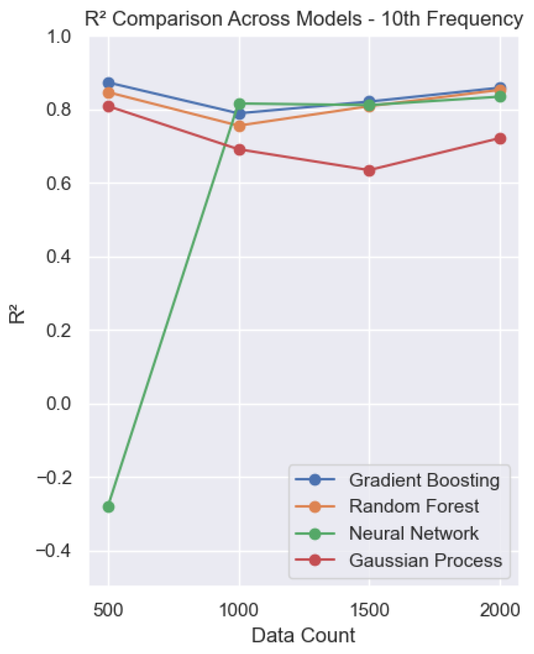
For the higher frequencies (4th–10th modes, Figure 6, Figure 7 and Figure 8), the neural network initially exhibits systematically low $R^2$ values when trained with the smallest dataset. This effect becomes more pronounced as the frequency increases. However, as the training set grows, the NN model improves significantly, reaching $R^2$ values of around 0.9. In these modes, both GB and RF show consistent and strong performance, with $R^2$ values typically ranging from 0.8 to 0.9. Conversely, the GPR model continues to underperform relative to the others, with $R^2$ values varying between 0.6 and 0.8.

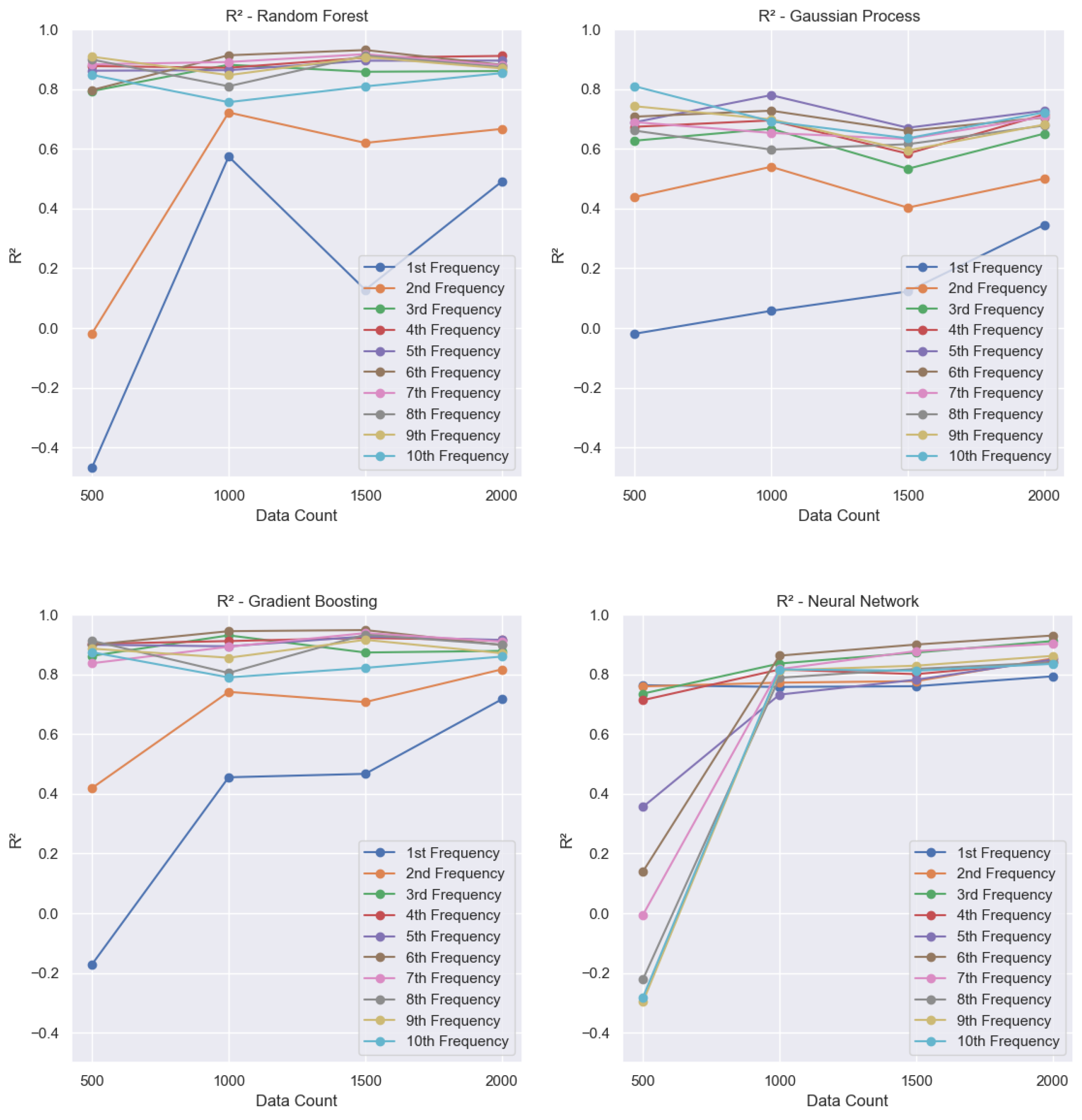
A consolidated view in Figure 9 highlights the following:

• Random Forest: For higher-frequency modes (from the 3rd to the 10th modes), the model achieves $R^2$ values between 0.8 and 0.9. For the smallest dataset, the second frequency has an $R^2$ close to zero, improving as the dataset size grows and reaching around 0.6. For the first mode, the $R^2$ is negative with the smallest dataset and increases with more data, but remains relatively low, stabilizing at around 0.5.
• Gaussian Process Regression: For the first frequency, the $R^2$ starts near zero and reaches only about 0.3. For the second frequency, it ranges between 0.4 and 0.5. For higher frequencies, the $R^2$ varies from 0.6 to 0.8. Overall, GPR is the model that consistently delivers the lowest performance across all frequencies.
• Gradient Boosting: For the higher frequencies (3rd to 10th modes), $R^2$ values range between 0.8 and 0.9. For the first frequency, the model starts with a negative $R^2$ and improves to approximately 0.7 as the dataset increases. For the second frequency, it starts at around 0.4 and reaches approximately 0.8 with larger training sets.
• Neural Network: For the first five frequencies, the $R^2$ values are initially low with the smallest dataset but increase consistently as the training set grows. This model achieved the best overall performance, including the first frequency, which reached $R^2$ values close to 0.8, higher than any other model.

4.2. Normalized Root-Mean-Square Error (NRMSE)

This section analyzes the normalized root-mean-square error (NRMSE) for the models. NRMSE provides a relative measure of prediction error, allowing comparison across frequencies and models as the training set size increases.

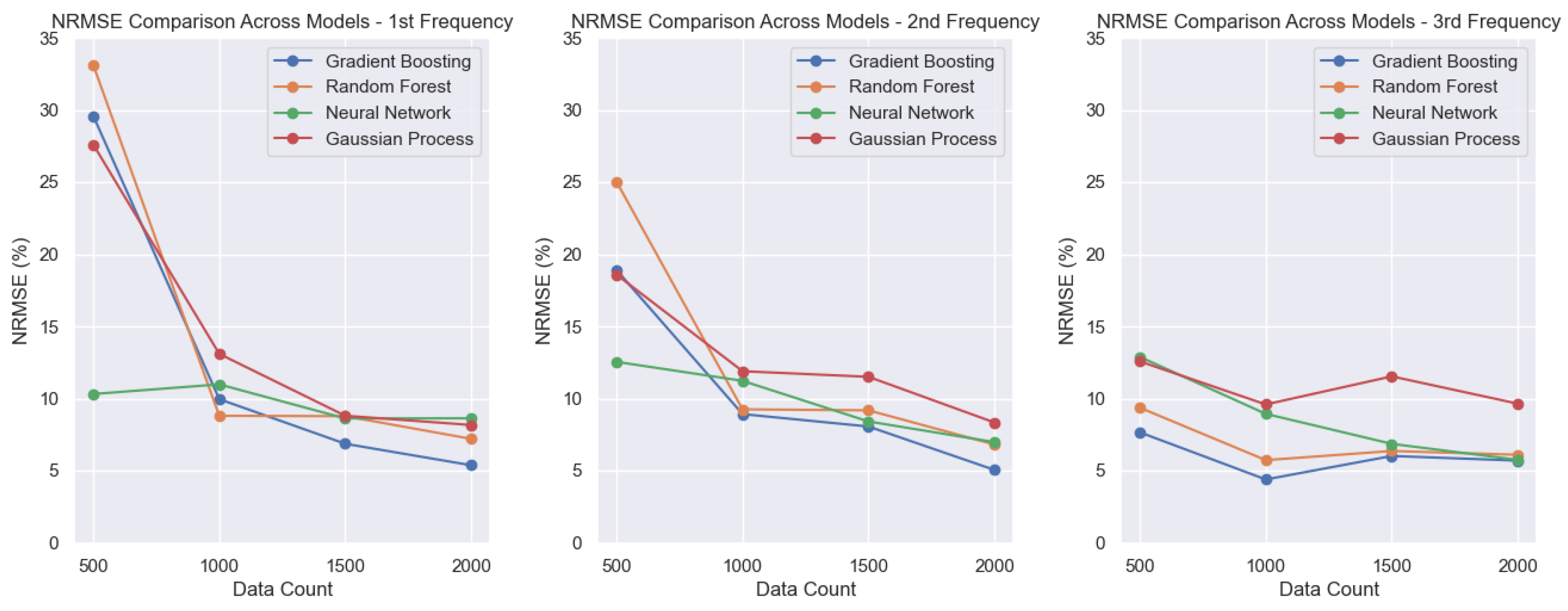
In the lowest modes (Figure 10), the neural network (NN) achieves the lowest NRMSE with the smallest dataset and continues to improve as the dataset increases. RF, GPR, and GB present high NRMSE values for the smallest dataset, around 30% for the first frequency and 20% for the second frequency, but their performance improves with larger datasets. For the first and second frequencies, GB stands out with the lowest error, around 5%. For the third frequency, GB, RF, and NN achieve similar NRMSE values close to 5%, while GPR once again shows the poorest performance among the models.

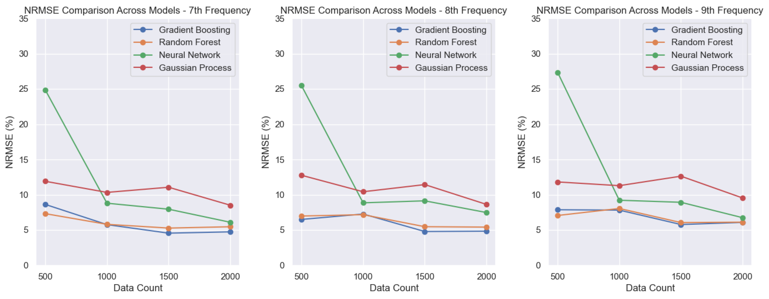
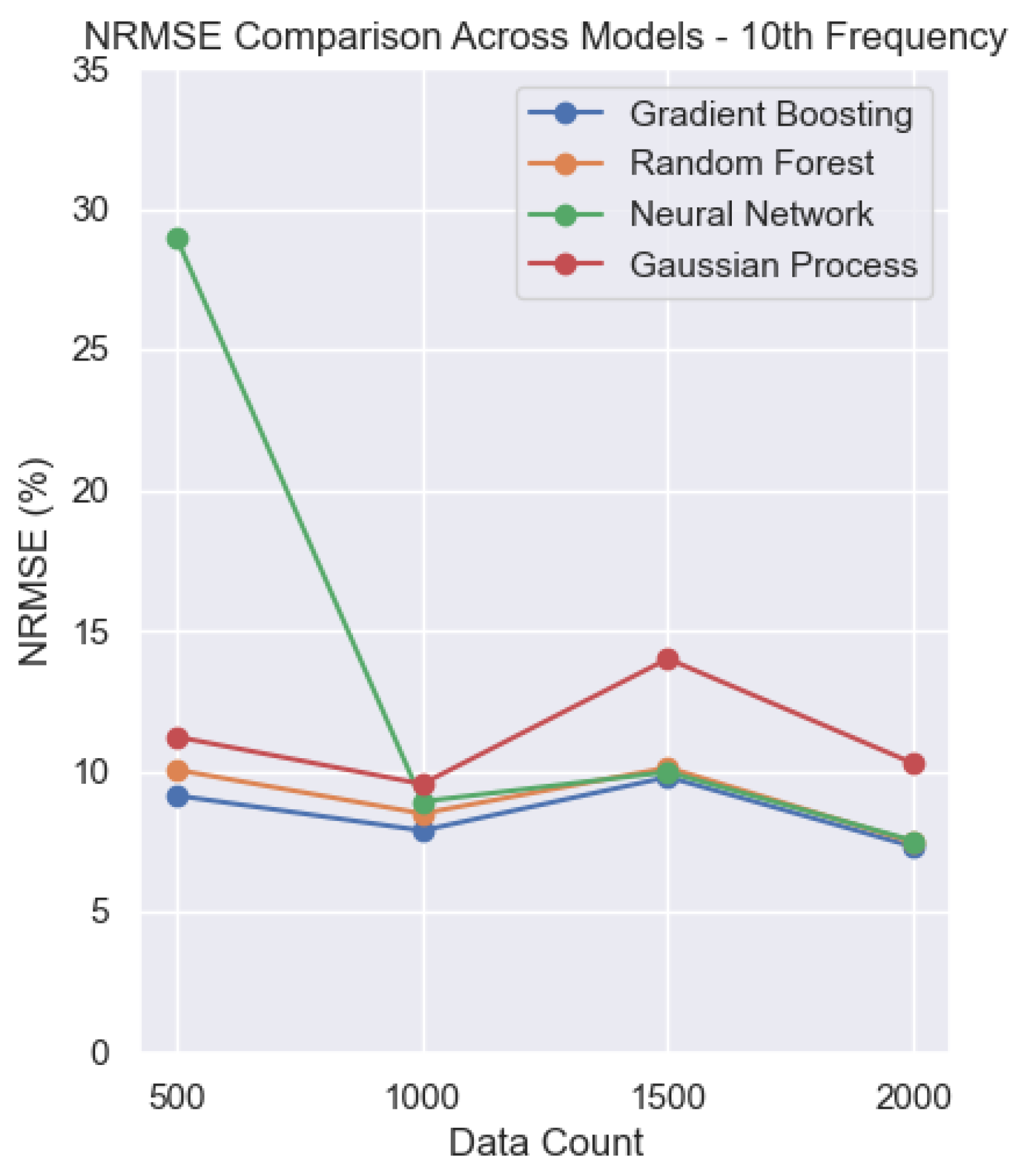
For higher frequencies (Figure 11, Figure 12 and Figure 13), the neural network (NN) shows higher NRMSE values for the smallest dataset, with errors increasing as the frequency rises. However, the NN’s performance improves steadily as the training set grows. Once again, the GPR performs worse than the other models, with NRMSE values of around 10%. The remaining three models achieve lower error ranges, reaching values close to 5%.

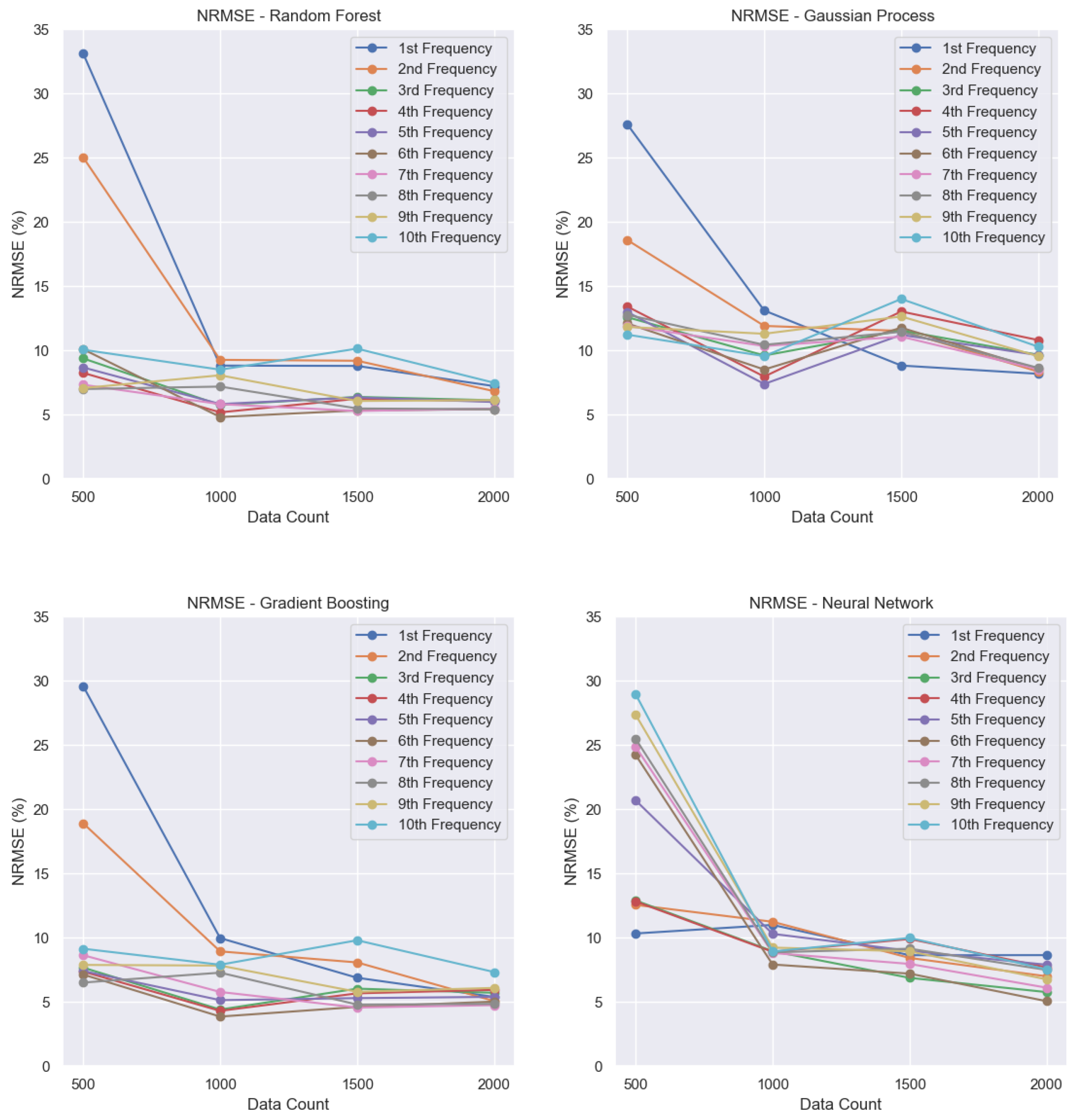
Figure 14 summarizes per-model error trends:

• Random Forest: The first and second frequencies show high errors with the smallest dataset but improve as the dataset size increases, ultimately reaching NRMSE values of around 5 to 8%.
• Gaussian Process Regression: Similarly, the first and second frequencies exhibit high errors with the smallest dataset, with final NRMSE values of around 10%. Overall, this model shows the poorest performance.
• Gradient Boosting: The first and second frequencies have high errors for the smallest dataset, but improve significantly, ending with NRMSE values between 5 and 7%. It is the model with the lowest NRMSE overall.
• Neural Network: Higher frequencies correspond to larger NRMSE values when trained with the smallest dataset; however, the model reaches NRMSE values of around 5 to 8% for most frequencies as the dataset grows.

Overall, the results demonstrate that Gradient Boosting achieves consistently strong performance, combining low NRMSE values and high $R^2$ scores across most frequencies and dataset sizes. Neural networks excel particularly in low-frequency modes, attaining high $R^2$ and low errors even with limited data, but require larger datasets to reach comparable accuracy at higher frequencies. Random forest shows steady improvements with increased data, providing competitive $R^2$ values and moderate NRMSE, though generally slightly behind gradient boosting and neural networks. Gaussian process regression consistently underperforms, with lower $R^2$ and higher NRMSE values, especially for small datasets and higher frequencies, indicating limitations in model flexibility or data efficiency for this problem.

The superior performance of boosting-based models observed in this study is consistent with previous findings in the machine learning literature for tabular and structured datasets. Gradient boosting methods are well known for their ability to capture complex nonlinear interactions through the sequential correction of residual errors, often leading to strong generalization performance [32]. Modern implementations such as XGBoost and LightGBM have repeatedly demonstrated state-of-the-art accuracy in regression tasks involving heterogeneous input features and moderate dataset sizes [33,34]. In contrast, Gaussian process regression, while theoretically attractive due to its probabilistic formulation and uncertainty quantification capabilities [35], can suffer from scalability limitations and reduced performance in higher-dimensional input spaces. Therefore, the observed dominance of the boosting approach in the present problem aligns well with previously published results and supports its suitability for surrogate modeling of complex engineering simulations.

The superior performance of the gradient boosting (GB) and neural network (NN) models can be explained by the physical characteristics governing propeller blade dynamics and by the modeling capabilities of these algorithms. Lower-order natural frequencies are primarily controlled by the global mass and stiffness distribution of the blade and vary smoothly with geometric and operating parameters. Neural networks are well-suited to approximate such smooth, high-dimensional relationships, which explains their strong predictive accuracy for the lowest modes. Higher-order frequencies are more sensitive to local geometric variations and rotational effects, leading to nonlinear and nonstationary input–output relationships. Gradient boosting models are particularly effective in capturing these localized behaviors, as they construct piecewise approximations that adapt to complex feature interactions. In contrast, Gaussian process regression tends to smooth these relationships and is more affected by the high dimensionality of the input space, which results in reduced predictive performance for this problem.

The data presented in this section were tabulated and are shown in

Table 9. Model performance for sample size $n=500$.

Natural Frequency	Model
	GPR		GB		NN		RF
	${\mathit{R}}^{\mathbf{2}}$	NRMSE (%)	${\mathit{R}}^{\mathbf{2}}$	NRMSE (%)	${\mathit{R}}^{\mathbf{2}}$	NRMSE (%)	${\mathit{R}}^{\mathbf{2}}$	NRMSE (%)
1	−0.0194	27.5969	−0.1713	29.5809	0.7633	10.3129	−0.4672	33.1072
2	0.4381	18.5841	0.4190	18.8975	0.7594	12.5406	−0.0183	25.0173
3	0.6270	12.5726	0.8616	7.6575	0.7351	12.8831	0.7931	9.3635
4	0.6735	13.4026	0.9018	7.3510	0.7133	12.8073	0.8767	8.2371
5	0.6886	12.9790	0.8989	7.3960	0.3557	20.6806	0.8614	8.6596
6	0.7074	12.0867	0.8985	7.1176	0.1391	24.2211	0.7966	10.0787
7	0.6893	11.9009	0.8369	8.6224	−0.0059	24.8538	0.8827	7.3133
8	0.6608	12.7576	0.9121	6.4922	−0.2220	25.4782	0.8985	6.9768
9	0.7424	11.8090	0.8857	7.8660	−0.2969	27.3472	0.9081	7.0529
10	0.8094	11.2126	0.8737	9.1268	−0.2819	28.9491	0.8472	10.0380

,

Table 10. Model performance for sample size n = 1000.

Natural Frequency	Model
	GPR		GB		NN		RF
	${\mathit{R}}^{\mathbf{2}}$	NRMSE (%)	${\mathit{R}}^{\mathbf{2}}$	NRMSE (%)	${\mathit{R}}^{\mathbf{2}}$	NRMSE (%)	${\mathit{R}}^{\mathbf{2}}$	NRMSE (%)
1	0.0573	13.0915	0.4550	9.9537	0.7576	10.9793	0.5738	8.8023
2	0.5396	11.8921	0.7410	8.9195	0.7719	11.2244	0.7215	9.2494
3	0.6671	9.5886	0.9302	4.3898	0.8359	8.9354	0.8812	5.7294
4	0.6950	7.9455	0.9111	4.2894	0.8160	8.8867	0.8712	5.1638
5	0.7795	7.3718	0.8935	5.1240	0.7319	10.2833	0.8630	5.8095
6	0.7274	8.4969	0.9442	3.8440	0.8623	7.8990	0.9130	4.8003
7	0.6530	10.3264	0.8920	5.7600	0.8171	8.7944	0.8905	5.8013
8	0.5973	10.4182	0.8043	7.2620	0.7884	8.8463	0.8092	7.1707
9	0.6985	11.2805	0.8553	7.8150	0.8130	9.2144	0.8465	8.0486
10	0.6917	9.5378	0.7896	7.8803	0.8163	8.9142	0.7560	8.4855

,

Table 11. Model performance for sample size n = 1500.

Natural Frequency	Model
	GPR		GB		NN		RF
	${\mathit{R}}^{\mathbf{2}}$	NRMSE (%)	${\mathit{R}}^{\mathbf{2}}$	NRMSE (%)	${\mathit{R}}^{\mathbf{2}}$	NRMSE (%)	${\mathit{R}}^{\mathbf{2}}$	NRMSE (%)
1	0.1223	8.8049	0.4666	6.8641	0.7599	8.6199	0.1278	8.7774
2	0.4029	11.5023	0.7069	8.0592	0.7770	8.4090	0.6197	9.1802
3	0.5329	11.5337	0.8729	6.0175	0.8726	6.8575	0.8578	6.3640
4	0.5836	13.0128	0.9214	5.6527	0.8003	9.8872	0.9049	6.2202
5	0.6703	11.1949	0.9267	5.2802	0.7817	8.9623	0.8948	6.3253
6	0.6596	11.7517	0.9480	4.5947	0.8995	7.1871	0.9305	5.3117
7	0.6326	11.0562	0.9378	4.5484	0.8776	7.9437	0.9166	5.2687
8	0.6153	11.4332	0.9327	4.7822	0.8178	9.1310	0.9121	5.4649
9	0.5945	12.6247	0.9153	5.7705	0.8287	8.9227	0.9069	6.0492
10	0.6349	13.9898	0.8214	9.7843	0.8119	9.9666	0.8089	10.1212

and

Table 12. Model performance for sample size n = All.

Natural Frequency	Model
	GPR		GB		NN		RF
	${\mathit{R}}^{\mathbf{2}}$	NRMSE (%)	${\mathit{R}}^{\mathbf{2}}$	NRMSE (%)	${\mathit{R}}^{\mathbf{2}}$	NRMSE (%)	${\mathit{R}}^{\mathbf{2}}$	NRMSE (%)
1	0.3454	8.1641	0.7163	5.3744	0.7931	8.6279	0.4905	7.2026
2	0.5002	8.3368	0.8165	5.0517	0.8530	6.9781	0.6665	6.8103
3	0.6509	9.6424	0.8781	5.6975	0.9112	5.7496	0.8602	6.1016
4	0.7150	10.7879	0.9140	5.9255	0.8419	7.6740	0.9108	6.0335
5	0.7275	9.6175	0.9147	5.3807	0.8492	7.8788	0.8951	5.9665
6	0.7046	8.5228	0.8979	5.0105	0.9298	5.0419	0.8809	5.4122
7	0.7075	8.5076	0.9094	4.7341	0.9024	6.0927	0.8796	5.4578
8	0.6778	8.6238	0.8988	4.8325	0.8398	7.4724	0.8733	5.4073
9	0.6810	9.5326	0.8704	6.0764	0.8615	6.7397	0.8690	6.1085
10	0.7220	10.2703	0.8592	7.3098	0.8349	7.5201	0.8533	7.4619

.

5. Conclusions

A data-driven framework was established to forecast the natural vibration frequencies of the propeller blades with high accuracy, providing a valuable tool for modern propeller design and optimization. By coupling a database of 1364 airfoil geometries with high-fidelity ANSYS simulations, the methodology captures the intricate effects of both geometric and operational variables on blade modal behavior.

A feedforward neural network implemented in TensorFlow/Keras was tuned via randomized search cross-validation over layer depth, neuron counts, learning rate, batch size, and optimizer type, yielding strong predictive performance. For higher-order modes, the model attained $R^2$ values above 0.90 and NRMSE below 8%, demonstrating the capability to explain the vast majority of the variance in the simulated data. Although predictions for the lowest frequency mode exhibited relatively greater error, overall accuracy highlights the effectiveness of machine learning as a surrogate for computationally intensive finite element analyses.

Compared to conventional simulation-only workflows, the proposed approach reduces runtime by orders of magnitude and readily scales to new design spaces, making it well-suited for iterative optimization loops in both aerospace and UAV applications. Additionally, the framework’s modularity enables integration with existing CAD and CAE pipelines and facilitates rapid evaluation of novel blade concepts.

Despite enabling large-scale data generation and efficient surrogate model training, the dataset and simulation framework present some limitations. From the initially generated configurations, only 1985 cases successfully converged, which may introduce a selection bias toward geometries that are numerically more stable and easier to mesh. The simulations rely on linear elastic, isotropic material assumptions and idealized boundary conditions at the hub; in particular, the blade root is modeled as a clamped boundary condition at the first airfoil section, representing an idealized hub–blade connection. The simulations do not account for fluid–structure interaction effects, which can influence modal characteristics under real operating conditions. In addition, the use of an automated tetrahedral meshing strategy with a fixed target resolution represents a compromise between accuracy and computational cost, and may limit the fidelity of higher-order modal predictions. Finally, the absence of experimental validation restricts direct assessment of the physical accuracy of both the numerical results and the trained machine learning models, highlighting the need for future studies incorporating experimental measurements.

Future research should focus on expanding the dataset, exploring alternative neural network architectures, and refining simulation parameters to enhance model accuracy, especially for lower-frequency modes. Such efforts will further consolidate the role of machine learning in advancing propeller design, thereby supporting the development of more efficient and sustainable aerospace and UAV propulsion systems.

References

1. Selig, M.S. Airfoil Coordinates Database. Available online: https://m-selig.ae.illinois.edu/ads/coord_database.html (accessed on 8 January 2026).
2. Brunton, S.L.; Noack, B.R.; Koumoutsakos, P. Machine learning for fluid mechanics. Annu. Rev. Fluid Mech. 2020, 52, 477–508. [Google Scholar] [CrossRef]
3. Montesinos López, O.A.; Montesinos López, A.; Crossa, J. Fundamentals of artificial neural networks and deep learning. In Multivariate Statistical Machine Learning Methods for Genomic Prediction; Springer: Berlin/Heidelberg, Germany, 2022; pp. 379–425. [Google Scholar]
4. Bongard, J.; Lipson, H. Automated reverse engineering of nonlinear dynamical systems. Proc. Natl. Acad. Sci. USA 2007, 104, 9943–9948. [Google Scholar] [PubMed]
5. Schmidt, M.; Lipson, H. Distilling free-form natural laws from experimental data. Science 2009, 324, 81–85. [Google Scholar] [CrossRef]
6. Sun, L.; Wang, J.X. Physics-constrained bayesian neural network for fluid flow reconstruction with sparse and noisy data. Theor. Appl. Mech. Lett. 2020, 10, 161–169. [Google Scholar] [CrossRef]
7. Lui, H.F.; Wolf, W.R. Construction of reduced-order models for fluid flows using deep feedforward neural networks. J. Fluid Mech. 2019, 872, 963–994. [Google Scholar] [CrossRef]
8. San, O.; Maulik, R.; Ahmed, M. An artificial neural network framework for reduced order modeling of transient flows. Commun. Nonlinear Sci. Numer. Simul. 2019, 77, 271–287. [Google Scholar] [CrossRef]
9. Karniadakis, G.E.; Kevrekidis, I.G.; Lu, L.; Perdikaris, P.; Wang, S.; Yang, L. Physics-informed machine learning. Nat. Rev. Phys. 2021, 3, 422–440. [Google Scholar] [CrossRef]
10. Raissi, M.; Perdikaris, P.; Karniadakis, G.E. Physics-informed neural networks: A deep learning framework for solving forward and inverse problems involving nonlinear partial differential equations. J. Comput. Phys. 2019, 378, 686–707. [Google Scholar] [CrossRef]
11. Liu, D.; Wang, Y. Multi-fidelity physics-constrained neural network and its application in materials modeling. J. Mech. Des. 2019, 141, 121403. [Google Scholar] [CrossRef]
12. Liu, D.; Wang, Y. A dual-dimer method for training physics-constrained neural networks with minimax architecture. Neural Netw. 2021, 136, 112–125. [Google Scholar]
13. Rao, C.; Sun, H.; Liu, Y. Physics-informed deep learning for computational elastodynamics without labeled data. J. Eng. Mech. 2021, 147, 04021043. [Google Scholar] [CrossRef]
14. Sliwinski, L.; Rigas, G. Mean flow reconstruction of unsteady flows using physics-informed neural networks. Data-Centric Eng. 2023, 4, e4. [Google Scholar] [CrossRef]
15. Doijode, P.S.; Hickel, S.; van Terwisga, T.; Visser, K. A machine learning approach for propeller design and optimization: Part I. Appl. Ocean Res. 2022, 124, 103178. [Google Scholar] [CrossRef]
16. Vardhan, H.; Volgyesi, P.; Sztipanovits, J. Machine learning assisted propeller design. In ICCPS ’21: Proceedings of the ACM/IEEE 12th International Conference on Cyber-Physical Systems; Association for Computing Machinery: New York, NY, USA, 2021; pp. 227–228. [Google Scholar]
17. Ahmad, F.; Kumar, P.; Patil, P.P.; Kumar, V. Design and modal analysis of a quadcopter propeller through finite element analysis. Mater. Today Proc. 2021, 46, 10322–10328. [Google Scholar] [CrossRef]
18. Kilikevičius, A.; Rimša, V.; Rucki, M. Investigation of influence of aircraft propeller modal parameters on small airplane performance. Eksploat. I Niezawodn. 2020, 22, 1–15. [Google Scholar] [CrossRef]
19. Dahal, C.; Dura, H.B.; Poudel, L. Design and Analysis of Propeller for High-Altitude Search and Rescue Unmanned Aerial Vehicle. Int. J. Aerosp. Eng. 2021, 2021, 6629489. [Google Scholar] [CrossRef]
20. Li, S.; Lee, S. A machine learning-based fast prediction of rotorcraft broadband noise. In Proceedings of the AIAA AVIATION 2020 FORUM, Virtual, 15–19 June 2020; p. 2588. [Google Scholar]
21. Legendre, C.; Ficat-Andrieu, V.; Poulos, A.; Kitano, Y.; Nakashima, Y.; Kobayashi, W.; Minorikawa, G. A machine learning-based methodology for computational aeroacoustics predictions of multi-propeller drones. In Proceedings of the Inter-Noise and Noise-Con Congress and Conference Proceedings, Virtual, 1–5 August 2021; Institute of Noise Control Engineering: Wakefield, MA, USA, 2021; Volume 263, pp. 3467–3478. [Google Scholar] [CrossRef]
22. Xie, K.; Chen, M.; Dong, W.; Li, W. A semi-analytic method for vibro-acoustic analysis of coupled propeller-shaft-hull systems under propeller excitations. Ocean Eng. 2020, 218, 108175. [Google Scholar] [CrossRef]
23. Uslu, S.; Bayraktar, M.; Demir, C.; Bayraktar, S. Innovative computational modal analysis of a marine propeller. Appl. Ocean Res. 2021, 113, 102767. [Google Scholar] [CrossRef]
24. Gypa, I.; Jansson, M.; Wolff, K.; Bensow, R. Propeller optimization by interactive genetic algorithms and machine learning. Ship Technol. Res. 2023, 70, 56–71. [Google Scholar] [CrossRef]
25. Soibam, J.; Aslanidou, I.; Kyprianidis, K.; Fdhila, R.B. Inverse flow prediction using ensemble PINNs and uncertainty quantification. Int. J. Heat Mass Transf. 2024, 226, 125480. [Google Scholar] [CrossRef]
26. Söderkvist Vermelin, W.; Mishra, M.; Eng, M.P.; Andersson, D.; Kyprianidis, K. Collaborative Training of Data-Driven Remaining Useful Life Prediction Models Using Federated Learning. Int. J. Progn. Health Manag. 2024, 15, 1–20. [Google Scholar] [CrossRef]
27. Soibam, J.; Scheiff, V.; Aslanidou, I.; Kyprianidis, K.; Fdhila, R.B. Application of deep learning for segmentation of bubble dynamics in subcooled boiling. Int. J. Multiph. Flow 2023, 169, 104589. [Google Scholar] [CrossRef]
28. Mählkvist, S.; Ejenstam, J.; Kyprianidis, K. Cost-sensitive decision support for industrial batch processes. Sensors 2023, 23, 9464. [Google Scholar] [CrossRef]
29. Netzell, P.; Kazmi, H.; Kyprianidis, K. Deriving Input Variables through Applied Machine Learning for Short-Term Electric Load Forecasting in Eskilstuna, Sweden. Energies 2024, 17, 2246. [Google Scholar] [CrossRef]
30. Alarcón, D.J.; Sampathkumar, K.R.; Paeschke, K.; Mallareddy, T.T.; Angermann, S.; Frahm, A.; Rüther-Kindel, W.; Blaschke, P. Modal model validation using 3D SLDV, geometry scanning and fem of a multi-purpose drone propeller blade. In Rotating Machinery, Hybrid Test Methods, Vibro-Acoustics & Laser Vibrometry, Volume 8: Proceedings of the 35th IMAC, A Conference and Exposition on Structural Dynamics 2017; Springer: Berlin/Heidelberg, Germany, 2017; pp. 13–22. [Google Scholar]
31. Ansys Mechanical, A. Theory Reference; Ansys Inc.: Canonsburg, PA, USA, 2017. [Google Scholar]
32. Friedman, J.H. Greedy function approximation: A gradient boosting machine. Ann. Stat. 2001, 29, 1189–1232. [Google Scholar] [CrossRef]
33. Chen, T.; Guestrin, C. XGBoost: A scalable tree boosting system. In Proceedings of the 22nd ACM SIGKDD International Conference on Knowledge Discovery and Data Mining, San Francisco, CA, USA, 13–17 August 2016; Association for Computing Machinery: New York, NY, USA, 2016; pp. 785–794. [Google Scholar]
34. Ke, G.; Meng, Q.; Finley, T.; Wang, T.; Chen, W.; Ma, W.; Ye, Q.; Liu, T. LightGBM: A highly efficient gradient boosting decision tree. In Proceedings of the Advances in Neural Information Processing Systems, Long Beach, CA, USA, 4–9 December 2017; Association for Computing Machinery: New York, NY, USA, 2017; Volume 30. [Google Scholar]
35. Rasmussen, C.E.; Williams, C.K.I. Gaussian Processes for Machine Learning; MIT Press: Cambridge, MA, USA, 2006. [Google Scholar]
Figure 1. Initial airfoil section geometry and processing steps.
Machines 14 00124 g001
Figure 2. Final 3D propeller blade geometry after lofting and refinement.
Machines 14 00124 g002
Figure 3. Example of the mesh generated for a propeller geometry. Tetrahedral elements and adaptive sizing were used to ensure mesh quality across varying blade sizes.
Machines 14 00124 g003
Figure 4. Modal shape corresponding to the first vibration mode of one of the analyzed geometries. The color scale qualitatively represents the displacement magnitude associated with this mode, with blue indicating regions of lower displacement and red indicating regions of higher displacement.
Machines 14 00124 g004
Figure 5. R2 × data count for the models—1st to 3rd frequencies.
Machines 14 00124 g005
Figure 6. R2 × data count for the models—4th to 6th frequencies.
Machines 14 00124 g006
Figure 7. R2 × data count for the models—7th to 9th frequencies.
Machines 14 00124 g007
Figure 8. R2 × data count for the models—10th frequency.
Machines 14 00124 g008
Figure 9. R2 × data count for each frequency and model.
Machines 14 00124 g009
Figure 10. NRMSE × data count for the models—1st to 3rd frequencies.
Machines 14 00124 g010
Figure 11. NRMSE × data count for the models—4th to 6th frequencies.
Machines 14 00124 g011
Figure 12. NRMSE × data count for the models—7th to 9th frequencies.
Machines 14 00124 g012
Figure 13. NRMSE × data count for the models—10th frequency.
Machines 14 00124 g013
Figure 14. NRMSE × data count for each frequency and model.
Machines 14 00124 g014